SIMULATION D'UN FLUIDE A LA SURFACE D'UN OBJET PAR
LA METHODE « SMOOTHED PARTICLE HYDRODYNAMICS »
par
Gilles-Philippe Paille
Memoire presente au Departement d'informatique
en vue de l'obtention du grade de maitre es sciences (M.Sc.)
FACULTE DES SCIENCES
UNIVERSITE DE SHERBROOKE
1*1
Library and Archives
Canada
Published Heritage
Branch
395 Wellington Street
OttawaONK1A0N4
Canada
Bibliotheque et
Archives Canada
Direction du
Patrimoine de ('edition
395, rue Wellington
Ottawa ON K1A 0N4
Canada
Your file Votre reference ISBN: 978-0-494-61447-1 Our file Notre r6f6rence ISBN: 978-0-494-61447-1
NOTICE:
AVIS:
The author has granted a
non-exclusive license allowing Library and
Archives Canada to reproduce,
publish, archive, preserve, conserve,
communicate to the public by
telecommunication or on the Internet,
loan, distribute and sell theses
worldwide, for commercial or
non-commercial purposes, in microform,
paper, electronic and/or any other
formats.
L'auteur a accorde une licence non exclusive
permettant a la Bibliotheque et Archives
Canada de reproduire, publier, archiver,
sauvegarder, conserver, transmettre au public
par telecommunication ou par I'lnternet, preter,
distribuer et vendre des theses partout dans le
monde, a des fins commerciales ou autres, sur
support microforme, papier, electronique et/ou
autres formats.
The author retains copyright
ownership and moral rights in this
thesis. Neither the thesis nor
substantial extracts from it may be
printed or otherwise reproduced
without the author's permission.
L'auteur conserve la propriete du droit d'auteur
et des droits moraux qui protege cette these. Ni
la these ni des extraits substantiels de celle-ci
ne doivent etre imprimes ou autrement
reproduits sans son autorisation.
In compliance with the Canadian
Privacy Act some supporting forms
may have been removed from this
thesis.
Conformement a la loi canadienne sur la
protection de la vie privee, quelques
formulaires secondaires ont ete enleves de
cette these.
While these forms may be included
in the document page count, their
removal does not represent any loss
of content from the thesis.
Bien que ces formulaires aient inclus dans
la pagination, il n'y aura aucun contenu
manquant.
1*1
Le 17 decembre 2009
lejury a accept e le memoire de Monsieur Gilles-Philippe Paille
dans sa version finale.
Membres du jury
Professeur Richard Egli
Directeur de recherche
Departement d'informatique
Professeur Djemel Ziou
Membre
Departement d'informatique
Professeure Virginie Charette
President rapporteur
Departement de mathematiques
Sommaire
Dans ce memoire, je presente une methode par particules pour la simulation de
l'ecou-lement d'un fluide contraint a se deplacer a la surface d'un objet. Plus precisement, la
methode Smoothed Particle Hydrodynamics sera utilisee pour discretiser le fluide ainsi que
pour l'animer. Un maillage approximant l'objet sur lequel le fluide s'ecoule sera utilise
pour le supporter et diriger son deplacement. Contrairement aux methodes precedentes,
une methode par particules permet l'independance du temps de calcul et la complexite du
maillage supportant le fluide. Elle permet egalement de suivre revolution de l'interface
li-quide/gaz et liquide/liquide sans procedure supplementaire. Des temps de calcul de l'ordre
du temps reel peuvent done etre obtenus sur des objets tres complexes.
Remerciements
Je tiens a remercier tous les membres de ma famille pour leur support tout au long de
mes etudes et qui m'ont encourage a entreprendre une maftrise. J'apprecie vraiment qu'ils
soient venus me rendre visite lors de mon sejour en France. Je remercie egalement tous les
gens que j'ai connus a Limoges, avec qui j'ai voyage et passe de tres beaux moments.
Je remercie mon directeur de recherche, le professeur Richard Egli, pour ses judicieux
conseils, ses idees et son ouverture d'esprit quant a 1'exploration de nouvelles pistes ayant
mene a la reussite du projet. Je tiens egalement a souligner l'aide de Benoit Crespin,
mon directeur de recherche lors de mon annee a l'Universite de Limoges, qui a
grande-ment contribue a l'elargissegrande-ment mon reseau de contacts en Europe et qui m'a accorde sa
confiance dans le developpement de mon projet de stage a Limoges.
Je remercie tous mes collegues, a Sherbrooke et a Limoges, pour les bons moments passes
en leur compagnie. En particulier, je remercie Khalid Djado pour tous les echanges que
nous avons eus, ses conseils et son sens de l'humour.
Table des matieres
Sommaire i
Remerciements ii
Table des matieres iii
Introduction 1
1 Notions Preliminaires 4
1.1 Smoothed Particle Hydrodynamics 4
1.2 Geometrie Riemannienne 8
2 Surface SPH 14
Conclusion 25
A Force geodesique 27
TABLE DES MATIERES
Introduction
L'ecoulement d'un fluide a la surface d'un objet est un phenomene souvent rencontre
dans la vie de tous les jours. Un premier exemple est la bulle de savon. La tension de surface
etant tres elevee, le liquide contenu a l'interieur de la mince couche de savon est contraint
a se deplacer dans un environnement s'apparentant a un espace en deux dimensions. Un
deuxieme exemple est le deplacement des nuages a la surface de la terre. Malgre l'epaisseur
des nuages, il est interessant de voir que leurs deplacements ne correspondent pas a un
ecoulement en trois dimensions traditionnel. lis sont plutot contraints a se deplacer dans
1'atmosphere terrestre. II en est de meme pour tous les autres astres ayant une atmosphere.
Cette contrainte nous permet d'appliquer une simplification importante avant de
ten-ter de simuler ces phenomenes. Etant donne que le mouvement du fluide dans une des
dimensions est negligeable, il est possible de reduire le probleme en eliminant un degre
de liberie. Cette reduction resulte en un ensemble d'equations s'apparentant aux equations
d'ecoulement d'un fluide en deux dimensions. Cependant, comme nous le verrons plus
tard, quelques details doivent etre considered lorsque 1'espace dans lequel le fluide se
de-place possede une courbure. Se situant au niveau theorique, cette simplification permet
d'economiser du temps de calcul, peu importe la methode de simulation utilisee.
Malgre sa grande presence, ce type de phenomene est tres peu exploite dans le
do-maine de l'infographie. Pour les methodes developpees jusqu'a present [15][14][13][5][4],
le temps de calcul reste tres eleve et depend fortement de la complexite du maillage
repre-sentant la surface, c'est-a-dire le domaine de simulation. Dans ce memoire, une methode
de simulation par particules est presentee pour resoudre les equations d'ecoulement d'un
fluide contraint a se deplacer a la surface d'un objet. Cette methode, nommee Smoothed
INTRODUCTION
Particle Hydrodynamics (SPH), permet l'independance entre le temps de simulation et la
complexity du maillage de la surface. Nous pouvons done obtenir des temps de calcul de
l'ordre du temps reel malgre la complexite de l'objet.
La surface servant a la simulation doit subir un pretraitement afin de simplifier
1'ap-plication des outils necessaires a la methode SPH. En effet, une etape de parametrisation
est necessaire afin d'adoucir les grandes variations geometriques de la surface. Cette etape
transforme la surface complexe en une surface reguliere, comme une sphere [8][10] ou un
plan [9][7], ou il est beaucoup plus facile d'appliquer les operateurs differentiels tels que
definis par la formulation SPH. Les distorsions creees par une telle transformation devront,
par contre, etre considered lors des calculs.
Pour cette raison, une parametrisation conservant localement les angles a ete
selection-nee. Tres utile, cette propriete nous permet une modification minimale des equations afin
qu'elles soient valides dans ce nouveau domaine. Ces transformations, nommees
applica-tions conformes, sont definies par un etirement infinite'simalement uniforme a chaque point
de la surface, ce qui nous garantit qu'un cercle infinitesimal defini sur la surface restera un
cercle dans le domaine parametrique. Cette deuxieme propriete nous sera tres utile lors de
la recherche de voisinage qui s'effectue traditionnellement par la definition d'un voisinage
circulaire autour d'un point.
Le probleme etant transpose dans ce nouveau domaine, il est maintenant simple de
si-muler l'ecoulement directement dans cet espace. L'application des forces et le deplacement
des particules seront ainsi effectues dans un seul et meme espace, facilitant
l'implementa-tion et la gesl'implementa-tion des variables. La posil'implementa-tion de chaque particule pourra ensuite etre
transpo-sed sur la surface a l'aide de l'application inverse, pour la visualisation de l'ecoulement.
Les contributions sont l'utilisation d'une methode par particules pour la simulation de
l'ecoulement d'un fluide a la surface d'un objet et l'independance de la simulation vis-a-vis
la complexite du maillage de l'objet sous-jacent. De plus, en tenant compte de la trajectoire
geodesique empruntee par une particule se deplacant dans une espace courbe, la distorsion
induite par la parametrisation de l'objet, presente dans les methodes par parametrisation
[15][13], est eliminee. Une simulation par particules permet d'autres formes de
visuali-INTRODUCTION
maillage. Un de ces types de visualisation est la simulation d'interfaces liquide/liquide ou
liquide/gaz, qui s'effectue de facon naturelle avec la methode SPH.
Le document est organise de la facon suivante : Le chapitre 1 introduit les notions
im-portantes a connaitre avant d'entreprendre la lecture du travail presente. II sera notamment
question de la formulation originale de la methode SPH et de la description mathematique
des concepts de base de la geometrie riemannienne. Le chapitre 2 presente l'article
Smoo-thed Particle Hydrodynamics on Triangle Mesh qui a ete soumis a la conference
Euro-graphics oil les articles acceptes sont publies dans le journal Computer Graphics Forum.
Quelques derivations techniques se trouvent en annexes pour ne pas encombrer inutilement
le texte, les references etant faites directement dans le texte aux endroits appropries.
Chapitre 1
Notions Preliminaires
Ce chapitre traitera des notions necessaires a la lecture de 1'article au chapitre 2. La
section 1.1 est une breve introduction a la methode Smoothed Particle Hydrodynamics dans
l'espace euclidien alors que la section 1.2 est une presentation des concepts cles de la
geometrie riemannienne.
1.1 Smoothed Particle Hydrodynamics
La methode SPH est tout d'abord une methode qui, a partir d'un ensemble discret de
points, permet d'evaluer les valeurs d'une fonction a chacun de ces points afin d'obtenir
une approximation de la fonction en tous points de l'espace. Cette approche nous permet
alors d'utiliser le calcul differentiel sur la fonction nouvellement definie. Elle a ete
inde-pendamment introduite par Gingold & Monaghan [6] et Lucy [12] en 1977..
Avant de considerer un ensemble discret, prenons une fonction / continue de R".
L'ega-lite 1.1 demontre que nous pouvons obtenir la valeur en un point en utilisant les valeurs au
voisinage de ce point [6].
1.1. SMOOTHED PARTICLE HYDRODYNAMICS
/(£).= lim f f(x')W(x-x',h)dR (1.1)
ou le noyau W satisfait aux conditions suivantes :
[ W{x-x',h)dR=l
JR
)imW(x-£,h) = 5{x-&)
ou
-,__,. f 1 six - x' = 0
I 0 sinon
En pratique, on doit ajouter quelques conditions au noyau etant donne qu'il sera
neces-saire que les calculs de derivees se comportent de fa?on satisfaisante [11]:
/ (x - x')W(x - x', h)dR = 0 Symetrie
JR
W{x-x*,h)\\\x-x'\\<h > 0 Positivite
W(x — x', h)\\\s-x'\\>h — 0 Support compact
ou la condition de support compact est seulement introduite pour reduire l'ordre de
com-plexite de 1'algorithme. Tel qu'illustre dans la figure 1.1, un exemple de noyau satisfaisant
a ces conditions est le suivant:
w
,..x 4 / (fc
2
-im
3
, «11*11 <fe
W[r,h) = —rz <
n1.1. SMOOTHED PARTICLE HYDRODYNAMICS
(a) (b)
figure 1.1 - (a) Voisinage circulaire d'une particule. (b) Exemple d'un noyau (h = 1)
D'une facon similaire, nous pouvons estimer la valeur du gradient et du laplacien par
les egalites suivantes.
V/(f) = lim / Vf(x')W(x-x',h)dR
A/(:r) = lim / A / ( f )W{x - x
1, h)dR
h^OjR
Mais ceci necessite de connaftre a l'avance V / et A / . L'ideal serait de pouvoir obtenir
le meme resultat en ne connaissant que / . Etant donne que nous avons impose la
condi-tion du support compact, il est possible d'utiliser l'integracondi-tion par parties pour obtenir les
egalites suivantes :
V/(f) = lim / f(x')VW(x-x',h)dR
h-*0
JRA/(f) = lim / f(x')AW{x-x',h)dR
h^OjR
(1-2)
(1-3)
Nous avons maintenant tous les ingredients necessaires pour definir les equivalents
dis-crets de ces formules. Nous devons tout d'abord laisser tomber la limite etant donne que
nous devrons avoir un support compact d'aire finie positive. Cette premiere modification
fera des equations 1.1, 1.2 et 1.3 des approximations. La deuxieme modification sera de ne
considerer qu'une quantite finie de points a l'interieur du support. II faudra done considerer
1.1. SMOOTHED PARTICLE HYDRODYNAMICS
que chacun des points Pj sont selectionnes au centre d'un volume Vj, pour en arriver aux
formules suivantes:
(m)=Y,W(x-x
j
,h)V
j
(1.4)
n
n
ou (f(x)) signifie 1'approximation de la fonction / .
Le seul detail restant a expliquer est la maniere de calculer le volume d'une particule.
Nous pouvons exploiter le fait que la methode sera appliquee a un phenomene physique
pour faire le parallele avec la masse et la masse volumique d'une particule. En effet, pour
un objet de masse m et de masse volumique p uniforme, nous avons que
V = = (1.5)
P
En assignant une masse rrij a chaque point Pj de notre ensemble discret, il est possible
de calculer son volume par 1'equivalent discret de la formule 1.5 :
Pj
Par cette demarche, nous avons simplement repousse le probleme car il nous reste a
connaitre la masse volumique pj de chaque particule pj. Heureusement, une astuce nous
permet de l'approximer par la formule 1.4 :
1.2. GEOMETRIE RIEMANNIENNE
n
n Pj
= y ^ m,jW(x — Xj,h)
n
A ce stade, nous sommes en mesure d'utiliser la methode SPH pour des applications
physiques. Nous n'avons qu'a assigner une certaine masse a chaque point, calculer la masse
volumique de chaque point pour ensuite effectuer des calculs sur un ensemble de valeurs
quelconques definies a chaque point.
1.2 Geometrie Riemannienne
Informellement, la geometrie riemannienne est l'etude des espaces munis d'une notion
de distance et des fonctions definies sur ceux-ci. Nous pouvons deja separer ce sujet en
deux sous-domaines, le premier etant l'etude de la structure de ces espaces et le deuxieme
etant la revision du calcul differentiel des objets definis dans ceux-ci. Cette section est une
simple introduction intuitive au sujet, de telle sorte que le lecteur puisse avoir une bonne
idee des concepts qui se cachent derriere les equations econcees dans l'article. Pour une
introduction plus detaillee au domaine, le livre de do Carmo [2] est conseille.
Le principal objet de la geometrie riemanienne est l'espace muni de sa notion de
dis-tance, qui est appele variete riemanienne. Un exemple simple d'une variete riemannienne
est la sphere dans 1R
3, sa notion de distance etant definie par la longueur d'arc euclidienne
d'une courbe tracee sur la sphere. Pour alleger la presentation et mettre en evidence
l'appli-cation de la theorie au probleme pose plus haut, cette section traitera seulement des surfaces
dans R
3, c'est-a-dire les varietes de dimension 2 plongees dans E
3.
1.2. G E O M E T R I E R I E M A N N I E N N E
(a) (b) (c)
figure 1.2 - Trois surfaces topologiquement differentes. Surfaces de genre 0 (a), 1 (b) et 2
(c).
S est le nombre de poignees qu'il faut ajduter a une sphere pour obtenir une surface de
topologie equivalente a S.
Pour etudier une surface S, la methode classique est d'utiliser des cartes locales. Une
carte locale u est une simple assignation de coordonnees de M
2a chaque point d'un ouvert
U de S. Ce processus d'assignation de coordonnees est appelee une parametrisation. Nous
pouvons ainsi recouvrir S avec un ensemble de cartes locales pour obtenir un atlas. Une
carte u et son inverse peuvent etre ecrits sous la forme mathematique suivante :
u
l= u
1(x
1, x
2, x
3)
u
2= u
2(x
1,x
2,x
3)
x
1= x
l(u
l,u
2)
x
2= x
2(u
l,u
2)
x
3= x
3(v},u
2)
ou les exposants representent des indices.
Un vecteur v tangent a la surface en un point p fait partie de l'espace tangent en ce point,
c'est-a-dire v E T
p. Cet espace vectoriel peut etre genere par deux vecteurs lineairement
independants gi,§2 € T
p. Ayant defini une carte locale u dans un voisinage local de p,
1.2. GEOMETRIE RIEMANNIENNE
coordonnees.
9\ =
h =
(dx
1(dx
1[du
2'
8x
2'du
1dx
2' du
2dx
3' du
1dx
3' du
2II est alors possible de trouver deux nombres reels v
1et v
2tels que v = v
lcj\ + v
2cJ2-Nous pouvons maintenant croire qu'il serait possible de travailler seulement avec les
com-posantes (v
l,v
2) sans jamais faire reference au vecteur original v qui est defini dans E
3.
Premierement, voyons comment calculer le produit scalaire de deux vecteurs tangents v et
w :
v-w = (t»Vi + v
2g
2) • {w
lg
x+ w
2g
2)
= v
1w
1(gi • gi) + v
1w
2(g
1• g
2) + v
2w
l{g
2• gi) + v
2w
2(g
2• g
2)
1 2= m
1v
- L.l
[v
1v
2]G
9I• 9i 9\- 32
#2 •
gI52 • g
2w
w
w
w
ou (G)ij — gij = 9v9i est appele le tenseur metrique. On note les composantes de l'inverse
deGpar(G-
1)
iJ= g
ij.
A ce stade, il devient utile d'utiliser la convention de sommation d'Einstein. II s'agit
simplement d'alleger la notation en rendant implicite la sommation lorsqu'un indice se
repete.
1.2. G E O M E T R I E R I E M A N N I E N N E
v%
9i =
Z )
v%9i
= v
x<7i + v
2g
2Pour le moment, nous avons trouve une facon de definir un vecteur tangent par rapport
a une base donnee, de telle sorte qu'on puisse calculer le produit scalaire en ne connaissant
que les coordonnees par rapport a cette base. Ce calcul est effectue a l'aide du tenseur
metrique.
Considerons maintenant un champ de vecteurs v tangents defini dans un voisinage de
p. II est possible de definir une derivee directionnelle d'un champ de vecteurs, nominee
de-rivee covariante, telle que le vecteur resultant soit toujours dans le plan tangent de p. Nous
devons considerer deux phenomenes. Le premier est que le vecteur normal a la surface peut
varier, ce qui entrainerait un vecteur qui n'est pas necessairement tangent. Le deuxieme est
que la base vectorielle peut aussi changer de point en point, ce qui entrainerait une
varia-tion des composantes du vecteur sans que le vecteur n'ait de variavaria-tions reelles. La derivee
usuelle dans la direction d'une ligne de coordonnee est definie de la facon suivante, sans
considerer le premier phenomene.
dv _ d(v
lgj)
dv
1^
{dg
xau
1av?
Nous pouvons maintenant definir la derivee covariante comme etant la projection de
la derivee directionnelle usuelle dans le plan tangent T
p. Le premier terme de 1'equation
1.6 etant deja un vecteur tangent, nous pouvons le laisser intact. Cependant, le deuxieme
terme peut produire une composante normale. On pose done T^, nommes les symboles
de Christoffel, comme etant les composantes telles que la projection du deuxieme terme
s'ecrive en fonction des vecteurs de la base vectorielle de T
p.
1.2. GEOMETRIE RIEMANNIENNE
PT
"
^
iS"
f
= r
^
fc
ou P
r pest la projection sur T
p.
Nous avons done une formulation mathematique complete de la derivee covariante dans
la direction d'une ligne de coordonnee, notee V^., par l'equation suivante :
dv
l_ , . _
9V>C iT^k \ *
Par linearite, nous obtenons la derivee covariante dans une direction quelconque w de
la facon suivante :
Les symboles de Christoffel encodent les variations de la base vectorielle et la
projec-tion sur le plan tangent. Etant donne qu'on se situe au niveau infinitesimal, la projecprojec-tion
peut etre vue comme une rotation definie par la variation du vecteur normal dans la
direc-tion de w. Bien que la definidirec-tion a l'aide de la rotadirec-tion soit plus naturelle pour la nodirec-tion du
1.2. GEOMETRIE RIEMANNIENNE
transport parallele d'un vecteur, elle porte a croire qu'il est necessaire d'avoir la
connais-sance de donnees extrinseques a la surface, les vecteurs normaux, alors que la derivee
covariante peut s'effectuer en ne connaissant que le tenseur metrique, qui est une donnee
intrinseque. La raison pour laquelle il est ideal d'avoir une definition intrinseque de nos
objets et de nos operations est de pouvoir effectuer tous nos calculs sur une carte locale
sans jamais faire reference a la surface originale.
L'obtention des symboles de Christoffel etant plutot technique et n'ajoutant pas a la
comprehension des concepts introduits dans cette section, ils seront simplement donnes
sans preuve par 1'equation suivante :
r
i
=9^ (dg
mjdg
mk_ dg
jk\
jk2 \du
kdui du
m)
Le dernier concept a voir avant de presenter 1'article est le transport parallele. II s'agit
d'une extension de la notion de parallelisme de l'espace euclidien aux surfaces. Pour le
definir mathematiquement, il nous faut tout d'abord selectionner une courbe 7 quelconque
sur notre surface. Pour chaque point de la courbe, selectionnons un vecteur v tangent a la
surface en ce point. On dit que le champ de vecteur ainsi defini est parallele s'il satisfait a
1'equation suivante:
V^
(t)v = 0 "
On peut voir qu'il s'agit simplement de la generalisation du fait qu'un champ de
vec-teurs paralleles dans l'espace euclidien ne varie pas de point en point. En particulier, si
la courbe satisfait a la condition Vj(t)j(t) = 0, on dit qu'il s'agit d'une geodesique. Elle
peut etre decrite comme etant une courbe ayant une acceleration nulle dans le plan tangent,
generalisant la ligne droite pour les surfaces.
Chapitre 2
Methode particulaire pour la simulation
de Pecoulement d'un flu ide sur un
maillage triangulaire
Cette partie du memoire presente 1'article Smoothed Particle Hydrodyamics on
Tri-angle Meshes. II s'agit d'un probleme propose par le professeur Richard Egli dans le but
de generaliser la methode particulaire Smoothed Particle Hydrodynamics a une surface de
genre 0 ou 1 representee par un maillage triangulaire. Sous la supervision de Richard Egli,
j'ai eu a developper la methode au niveau theorique, a l'implementer et a rediger 1'article
qui constitue ce chapitre.
Nous proposons une methode permettant la simulation d'un fluide a la surface d'un
objet en temps reel. Le principe est de transformer la surface en un espace plus regulier,
comme la sphere ou le plan, et de resoudre les equations de Navier-Stokes sur ces nouveaux
domaines en considerant les deformations induites par la transformation. L'espace regulier
choisi dependra de la topologie de la surface originale.
L'article est divise en deux parties. La premiere est la presentation des methodes de
parametrisation d'une surface. Une breve description des methodes existantes permet de
bien definir l'estimation des metriques, des connexions et des vecteurs caracterisant la
pe-riodicite du domaine parametrique. La deuxieme partie constitue le coeur de 1'article. Une
breve revue de la methode SPH classique est presentee avant de la generaliser aux surfaces
de genre 0 ou 1. Une attention particuliere est portee au calcul des distances et au calcul
de la trajectoire geodesique qu'emprunte une particule se deplacant dans le domaine
para-metrique. La section traitant de la force geodesique presente des formules sans derivation
detaillee. L'annexe A presente done le calcul detaille de ces formules pour le cas du plan et
de la sphere.
EUROGRAPHICS 'Ox / N.N. and N.N. Volume 0 (200x), Number 0 (Editors)
Smoothed Particle Hydrodynamics on Triangle Meshes
Gilles-Philippe Paille, Richard Egli Centre MOIVRE, Departement d'Informatique Universite de Sherbrooke, Sherbrooke, Quebec, CANADA
Abstract
We present a particle-based method for solving Navier-Stokes equations on the surface of objects of genus 0 and 1. When the mesh is conformally mapped to a domain of constant curvature, the problem is greatly simplified due to the regularity of the new domain and the uniform stretching property of conformal maps. We adapt the Smoothed Particle Hydrodynamics method to work in this framework and we reformulate the momentum equation so that it takes into account the geodesic path taken by the particles. A particle-based method allows the simulation time to be independent of the underlying mesh resolution and offers a natural way to compute free-surface flows. We therefore achieve real-time simulation without-artifacts caused by the parameterization of the triangle mesh.
Categories and Subject Descriptors (according to ACM CCS): 1.3.7 [Computer Graphics]: Three-Dimensional Graphics and Realism—Animation
1. Introduction
Fluid flows on the surface of an object can be observed at very different scales. Clouds moving across the surface of the earth can be well approximated by a fluid flowing on a sphere. At a smaller scale, soap films are another example of liquid constrained to move on a curved domain. But the com-plexity of such phenomena can be simplified by considering that the fluid is moving on a curved 2D domain instead of a small subset of a full 3D Euclidian domain. Such simplifi-cations allow us to remove a degree of freedom, simplifying equations and saving computation time.
Mesh methods for solving Navier-Stokes equations on an object represented by a triangular mesh have been devel-oped, but they suffer from being very expensive to compute and depend heavily on the underlying mesh. We propose a particle approach, namely the Smoothed Particle Hydrody-namics method (SPH), to solve these equations in real time without explicit dependency on the triangle mesh. The re-sulting method is very simple and requires only minor mod-ification of a standard 2D SPH simulation to be suitable for curved objects of genus 0 and 1.
The simulation uses the uniform stretching property of conformal mapping to simplify equations in the SPH formu-lation. By first mapping the mesh conformally to a regular
domain, the computations are entirely done in the parame-ter domain and the particles can be easily transposed to the original object space for visualization.
Our contribution is the use of particle-based real-time simulation for fluid flow over a surface, allowing the sim-ulation to be independent of the complexity of the mesh. By taking into account the geodesic path of a moving particle, we remove distortions resulting from the parameterization of the mesh. A particle-based simulation allows for simple sur-face tracking, which offers new possibilities for other forms of visualization, like free surface flows, all in a single unified method.
The paper is organized as follows : Section 2 reviews ex-isting work on conformal parameterization, SPH and flow on surfaces. Section 3 explains the offline computations that need to be performed before doing the simulation. Section 4 recalls the basics of the SPH method that works on Eu-clidean domains. Then, Section 5 extends the SPH method to work on non-Euclidean domains, which is our main con-tribution. Results are then presented in Section 6 showing the independence of the mesh resolution and free-surface flows on mesh. Our conclusions are given in Section 7.
2. Related Work
2.1. Conformal parameterization
Discrete conformal parameterization has been extensively studied in the past decade. We will concentrate on methods that map genus-0 objects to the unit sphere and genus-1 ob-jects to the plane.
Let us first enumerate sphere parameterization methods. [AHTK99] and [HAT* 00] describe a technique in which the object is first mapped to the plane, then stereographi-cally projected to the sphere to obtain the conformal map-ping. [GtY02], [Gu03] and [GWC*03] describe a technique in which the Gauss map is taken as the initial approximation, then updated with a diffusion process to minimize an energy functional. The resulting map is then conformal. [LH07] up-grade this method with a new initial map and a modified diffusion process that speeds up convergence.
Global conformal parameterization of genus-1 objects is done by [GtY02], [Gu03] and [GY03] using differential one-forms defined on each edge of the mesh to solve two lin-ear systems. The resulting set of one-forms can then be op-timized for some desired properties using the method de-scribed in [JWYG04]. Cutting the mesh along the homology basis, it can then be unfolded to a plane homeomorphic to a disk by integrating one-forms.
2.2. Smoothed Particle Hydrodynamics
Smoothed Particle Hydrodynamics was introduced by [GM77] and [Luc77] but the first application of this method in the computer graphics community was made by [DG96] for simulation of deformable bodies. [SAC* 99] then used it to simulate lava flows, including heat transfer and non-constant viscosity. [MCG03] used SPH to simulate fluid in-teractive time, including surface tension force. We have cho-sen to use this last formulation of SPH due to the simplicity of the formulas and the stability of the overall simulation.
2.3. Surface flows
The concept of fluid flows on surfaces was introduced to the computer graphics community by [Sta03], who computed a local parameterization for each quadrilateral patch on which he solved the Navier-Stokes equations. Transition functions were defined between each pair of neighboring patches to transfer fluid properties across the entire mesh. Distortions are created by a misinterpretation of the advection term, re-sulting in a fluid that does not follow a geodesic path. [SY04] did the simulation directly on the mesh using an adaptation of the semi-Lagrangian method introduced by [Sta99], elim-inating distortion with parallel transport of the velocity vec-tor in the backtracing step. Their method simulates incom-pressible and inviscid fluid flow by solving the Poisson equa-tion and advecting fluid properties at each iteraequa-tion.
[LWC05] conformally parameterized the mesh to solve
the Navier-Stokes equations on the parameter domain. The same misinterpretation of the advection term as in [Sta03] deviates the fluid from the geodesic path. [ETK*07] used the simplicial complex and the chain complex paradigm to translate equations into chain operations. [FZKH05] adapted the Lattice-Boltzmann method by using the tangent space at each vertex to project neighboring lattices on it.
In computer animation with particles, [DE09] used a par-ticle system to visualize a velocity field resulting from a fluid simulation. The particles need some velocity correction to avoid interpenetration and two different steps are needed to do the simulation and the visualization. The simulation step is Eulerian and therefore also depends on the resolution of the mesh.
The computational time of these simulations depends heavily on the complexity of the mesh, which makes them difficult to use for real-time applications. Particle simulation removes this dependency. In addition, it allows for new visu-alization techniques that would require additional processing steps using mesh simulation methods.
2.4. Contribution
Below is a list of the contributions made by the method we present in this paper.
• Particle-based method for surface flows • Correct treatment of the advection term • Simulation independent of the mesh resolution 3. Parameterization
Particle-based simulation would be very hard to perform di-rectly on the mesh because of the curvature. The solution that we propose is to transform the mesh to a more regu-lar shape, like a plane or a sphere, via a parameterization process. Many different mapping techniques exist. A sub-set of these techniques, called conformal maps, uniformly stretch an infinitesimal neighborhood of each point of a sur-face. This ensures angle preservation and avoids shearing transformation, which are very nice properties to have when working in the parameter domain. Conformal maps are pre-ferred over exponential maps defining local isometries be-cause the latter approach requires too many different maps to cover the mesh efficiently, whereas the former only needs one map.
When expressed in a conformal domain, Navier-Stokes equations only need to be slightly modified to remain valid in the new domain. The uniform stretching also ensures that a small circular neighborhood is kept circular in the new do-main, which will be very useful for the neighbor search pro-cess of SPH.
We will only use global mapping, since it removes the need to do a mesh segmentation and compute patch tran-sition functions. Genus-0 surfaces are mapped to a sphere 17
while genus-1 surfaces are mapped to a periodic plane. We will first describe the mapping process, then compute some metric information about these mappings that is needed dur-ing the fluid simulation. It is to be noted that everythdur-ing in this section is done offline.
For what follows, M is a mesh with vertices {v;}, edges {e/y} and triangles
{fijk}-3.1. Genus-0 surfaces
Since a genus-0 surface is homeomorphic to a sphere, a bi-jective map can be computed between the two surfaces. This is done by the method described in [GWC'03] and [LH07], which we will briefly review here.
A conformal map between two genus-0 surfaces is equiv-alent to a harmonic map. Since the latter can be computed using a simple iterative minimization procedure, we can use this same procedure to compute a conformal map. The map-ping is done by first assigning an initial position <f>o(v;) to each vertex of the mesh on a sphere, then iteratively updat-ing the new position to finally get a conformal map. The conformal map is obtained when the mapping minimizes an energy functional of (p on M, described in Equation I below.
E(M)= f |Vcp(x)|2</M (1)
JM
The energy is minimized when the equation Acp = 0 is satisfied. The iteration process is conceptually the same as heat diffusion on the surface. This diffusion is done until we reach a steady state of the diffusion equation (Equation 2).
^ = -Aq»(v,) (2) The initial map can be simply the Gauss map or a
stere-ographic projection of a planar graph representation of the mesh, the latter eliminating fold-over problems. From this initial guess, we iteratively move each vertex in the direc-tion of the tangential component of the Laplacian A until it converges. The Laplacian on a mesh is defined by Equation 3.
Ar<p(v,-) = PtfV()£*,y(q>(v,)-<p(v;)) (3)
e'i
where P«>(v,) 's m e projection operator on the tangent plane of the sphere at position <p(v;) and k-,j is defined by the cotan-gent formula (Equation 4).
kij = -(cotaij + cotfrj) (4)
where a;y and P;y denote the angles opposite to the edge e/y in the two triangles adjacent to e;y.
At every iteration, we need to normalize <p(v,) to ensure that the whole map stays on the sphere.
3.2. Genus-1 surfaces
For genus-1 surfaces, we need to proceed differently. We will briefly review the technique described by [GY03] for genus-1 surfaces. The mesh M will be cut in a way that al-lows it to be unfolded to a flat plane, obtaining the funda-mental domain. The new position of each vertex on the plane is found by first solving linear systems of one-forms defined on each edge, then integrating the resulting one-forms on the fundamental domain. A one-form co is an assignment of a real value 0)/y to each edge e;y of Msuch that C0/y = — coy;. By identifying the cut edges, we obtain a periodic plane that is topologically the same as the original object.
Obtaining the fundamental domain is done by a collapsing procedure, see [Gib77]. Selecting an arbitrary initial triangle of the mesh and labeling it as visited, all neighbor triangles are recursively visited, with no prescribed order, until ev-ery triangle has been labeled. During this procedure, some neighbors will already be visited. In this case, the edge adja-cent to the two triangles is marked as a potential fundamental domain border. We only collapse triangles because we need the original edges to build the fundamental domain border. After the collapsing procedure, we obtain a set of potential edges. Dangling edges are recursively removed until none remain. The edges are then cut to create the fundamental do-main to be unfolded. The resulting border is not necessarily minimal and does not need to be minimal.
Every genus-1 surface has two generators for a homol-ogy basis So a nd B\ that can be found from the set of
bor-der edges using standard computational homology methods [KMM01]. The basis {Bo,B\} is simply a set of edges rep-resenting loops that cannot be contracted to a point on the surface.
The goal is to find a pair of one-forms (a, T) SO that we can find the new parameters (i;,!;) associated with every vertex
Vj.
The next step is to solve the two linear systems in Equa-tion 5, the unknowns being the two one-forms (i)» and (0,^ defined on each edge e^ of the mesh.
»yt + <4/ + »// = 0. Y//W 6 M
X ^ Q ) > = 0,Vvy6M (5) eJt€M
eitEBi
Choosing Gjk = u)^ as being the one-form correspond-ing to the first parameter domain coordinate, we are ready 18
to compute the second coordinate one-form T,*, which is a linear combination of the two known one-forms.
0 < K 1
The coefficients y, are found by solving a small linear sys-tem of equations, defined by Equation 6.
Wy=c (6)
where c and W are defined respectively by equations 7 and
s ^ ^ f e
(a)*
^•/ Ah,€M ">kl wlm wmk< < ,
"it
A»,ewwhere A4;,„ is defined by Equation 9 [Gu03].
Gkl Vim Gmk (7) (8) 1 2(b2+c2) a2 + b2-c2 a2+c2 Mk/m = -^-\b2+a2-c2 2(c2+a2) b2 + c2-a2) 24A
V
+ a2_
62 c
2+b
2-a
22(a
2 +b
2)J
(9) where/I is the area of the triangle /«,„, a = \\eki\\,b = ||e/,„||andc=||e,„t||.
Having obtained a one-form corresponding to each pa-rameter, we are ready to compute the final parameterization by integrating the one-forms over the fundamental domain of M. By choosing an arbitrary initial vertex to be at the ori-gin (0,0), we find the coordinates of the neighbor vertices by Equation 10, using a flooding procedure similar to the fundamental domain computation.
fay.'y) = (*<•>'<•)+ (o/y,T//) (10)
for every unknown vertex of coordinates (SJ,IJ) neighbor-ing a known vertex of coordinates (sj,tj).
3.2.1. Fundamental parallelogram
The unfolding of the fundamental domain can send two neighboring points very far apart. The periodicity of the fun-damental domain is thus an important concept to take into account when computing distances on it, see section 5.2. For
(c)
Figure 1: Periodicity of the domain, a) The mapped mesh, b)
The fundamental domain, c) The periodic structure of the do-main with fundamental parallelogram vectors joining equiv-alent points.
this purpose, we will define two vectors forming the funda-mental parallelogram [GY03]. These are a pair of indepen-dent vectors representing the shortest non-null translations needed to get back to an equivalent point on the parameter domain (see Figure 1).
This equivalence relation is expressed by Equation 11: two points are equivalent if they are separated by an integral linear combination of the fundamental parallelogram vectors
bo and 6).
p = p + ibo+jb\,Vije'. (11) These vectors are simply computed by integrating one-forms over the homology bases using Equation 12.
= £ (Oy*,Xyt) (12)
3.3. Metrics
A mapping generally induces local deformations that need to be taken into account in doing computations on the parame-ter domain. A metric g is a bilinear function which takes as input two tangent vectors and returns a scalar, generalizing the dot product in Euclidean space. Since a bilinear function can be represented by a matrix, we can build a 2x2 matrix with components g,y called the metric tensor. We denote the components of the inverse of the metric tensor as g11.
Since a conformal map only locally induces a uniform stretch, the metric tensor is proportional to the metric tensor of the parameter domain, which is, in our case, the identity matrix. The constant of proportionality is caljed the confor-mal factor and is denoted by X . It is generally different for every point on the object and it is the only value that will be needed to compute lengths and areas in the parameter do-main.
In the discrete setting of an object represented by a tri-angle mesh, a conformal factor will be computed for ev-ery vertex v, of M. Concretely, A. represents the ratio of a unit of length on the mesh to a unit of length on the pa-rameter domain. They are computed once the papa-rameteri- parameteri-zation procedure is done using the formula in Equation 13 from [JWYG04],
Xr 1
Ik
(13)where n is the number of incident edges to the vertex v,-. 3.4. Affine connections
Differential calculus on manifolds involves the notion of par-allel transport for vector quantities. Parpar-allelism on a curved surface needs to be defined using the affine connection of the metric [dC92]. This is a map that encodes changes in the basis used to represent a vector from point to point. They are needed to compute directional derivatives of a vec-tor quantity like the velocity of a particle, see section 5.3. For a surface admitting a Riemannian metric g, as in our case, the connection is represented with the Christoffel sym-bols, as defined in Equation 14. We make use of the Ein-stein summation convention where repeated indices are im-plicitly summed over. For clarity, derivatives are denoted by
dgmj 3
dj = lnAwj — lnA.v,,0 < j < n (17)
4. SPH Basics
SPH is an approximation method that defines a continuous function from an unorganized set of points. To each point in the set is associated a mass mj and a density py. To
ap-proximate the function at a position r, a convolution is done with the surrounding points inside a radius h, the smoothing
length. The value of a properly A contained at each point
is weighted by a the kernel function W and summed over a local neighborhood.
(m)
- I ^nr-n,h)
jeN(r) PJThe masses mj are given while the densities py need to be computed using Equation 18 before being able to compute any other property.
= Wi)) j€N(n) Vj -- X mjW(r,-rj,h) J£N(n) (18) 4.1. Derivatives
Having defined a continuous function over the whole space, it is now easy to define the gradient and the Laplacian of any property A. After some manipulations, one can show that the discretized gradient and Laplacian are given by equations 19 and 20.
r",
jk~- • fikgrnj + djgmk - Smgjk) (14)For a conformal map, the expression of the connection is pretty simple. The components of T being a combination of the components of V In A, we only need to compute this gradient at each vertex in the parameter domain. For a vertex v; having n neighboring vertices {wj}, we can approximate the gradient with the pseudoinverse formula in Equation 15:
V\nXVi = {WTW)~lWTd (15)
where the jth row Wj. of the matrix W and d are defined as in equations 16 and 17. W<. Vj — V;,0 < j < n (16) V{A(r))= X ^-VWCr-rjJ) (19) A< 4 ? ) ) = - £ ^-AW(r-rj,h) (20) j€N(f) Py 4.2. Kernels
The kernel functions used in the constitutive equations of SPH need to follow some rules to give a good approximation of the desired result. These properties are as follows: • JW(r,h)dV= 1 Unity
• JW(r,h)rdV = 0 Symmetry • W(r, h) 11|?|| <h > 0 Non-negativity
• ^'(':,^)||I?||>A = 0 N " " outside neighborhood
WX&'fr--?
The new set of equations (see [ARI89]) benefits from the nice properties of the global conformal mapping.
PD 7 r V p - ^ A i ? + G(U) + ^
viscosity geodesic external (21)
(a) (b)
Figure 2: Particle distribution. A uniform particle
distribu-tion on the surface (a) induces a non-uniform distribudistribu-tion in the parameter domain (b) due to the distortions caused by the parameterization.
where the last condition is only introduced to get an algo-rithm of linear complexity.
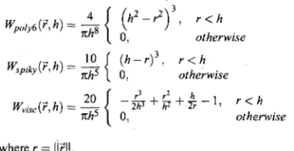
The kernel functions need not be the same for every com-putation. For instance, three different kernels will be used for each property. These functions are chosen for their simplic-ity, speed of computation and stability. Density computation uses Wpoiys while the pressure and viscosity computations use Wspjky and WVjSC, respectively.
W, polyS (?,*) = nhs 10 WvisC(7,h) = nh5 20 -r2 (h-r)\ 0, , r <h otherwise r <h otherwise nh5 1 0 2A3 r/ ? + 2 ?- 1' r<h otherwise where r
-The coefficients in front of each kernel are necessary to ensure the unity property. They are only valid in 2D and thus are valid for our application on surfaces.
5. SPH on a surface
The first thing to do in order to simulate fluid flow on the surface of an object is to adapt the Navier-Stokes equations. Since the particles will be moving on the parameter domain, the distortions caused by the parameterization must be con-sidered (see Figure 2). They appear in the computation of the gradient and the Laplacian, and of the path taken by par-ticles.
From now on, we need to be careful with the properties we are manipulating, since there are two different spaces in which they can "live": the surface and the parameter domain. Properties that live on the parameter domain will be written
A and those that live on the surface will be written A to avoid
any confusion.
We see that the only differences with the original Navier-Stokes equations are the use of the conformal factors X and the addition of the geodesic force. This force comes from the parallel transport of the velocity to ensure that a particle will follow a geodesic path on the surface. Details about this force will be given in Section 5.3.
Information on metrics and connections is only known at vertices of the mesh. Since a particle is necessarily contained in a triangle of the mesh, these properties can be found by doing barycentric interpolation of the values contained at each vertex.
5.1. Corrected formulas
First, we have already pointed out that a conformal param-eterization maps circles to circles of different radius. This means that we can still use a circular neighborhood in the pa-rameter domain, but we need to change the smoothing length by some factor. Noting that a unit of length in the parame-ter domain is stretched by a factor of X to be valid on the surface, we need to define the new radius by Equation 22.
h
'
=h
(22) where h is the global smoothing length, Xj is the stretch fac-tor at the position of particle j and hj is the local smoothing length of particle j .We can also point out that if lengths are stretched by a fac-tor X, areas will be stretched by a facfac-tor A.2. For this reason,
the area occupied by a particle in the parameter domain is computed by Equation 23.
PA2
(23)
As we wish to do every computation in only one domain and Equation 21 is written in such a way that the differential operators are to be applied in the parameter domain, the new SPH formulation will be described by Equation 24.
(AC
jeN(r) YJKJ
d{r,rj).
\X(r) (24)
where d(r,rj) means the vector representing the shortest straight path between r and ?j. This subtlety will be fully discussed in Section 5.2.
Given this new formulation, it is easy to define the den-sity, gradient and Laplacian on the parameter domain using equations 25, 26 and 27.
jS,= X Tin^n,rj),h,j)
jeN(r) Kj • (25)iv</!(n)> = i I ^i^n3(n,rj),hij) (26)
Ki Ki jeN(r) Pj'Kj -^A(«(?,)> = 1 X ^LiSj-wwidftWhij) Ki Ki jeN(f) PJKj (27) where h-,j = (ft,- + hj)/2 and pj = kp"j, with k being a con-stant.5.2. Distance computation
As explained in Section 3.2.1, the distance between two points on the global conformal domain needs to take into consideration the periodic structure of the domain. Due to . this periodicity, multiple straight paths can be drawn be-tween two points on the parameter domain, as illustrated in Figure 1. Only the shortest path is relevant to the computa-tion and this is the path that will be used for the SPH formu-lation.
For genus-0 surfaces, the mesh is mapped to a sphere. In this case, the Euclidean distance is a good approximation of the real distance and naturally gives the shortest distance.
For genus-1 surfaces, the mesh is mapped to a periodic fiat domain. We need to look for the closest translated copy of a particle pj around the particle position p,. This is done by translating pj by integer values of the fundamental parallel-ogram vectors defined in Section 3.2.1 and taking the differ-ence relative to the closest translated position of the particle. Mathematically, this path vector is defined by Equation 28.
d{p\,p2)=dij, \\dij\\ = min 114/11 (28)
where d,j = pi - p\ + ib\ + fbi
5.3. Geodesic force
The path of a free particle moving on a manifold without force acting on it will have zero geodesic curvature since, by definition, the geodesic curvature is the acceleration of a curve in the tangent space of the manifold. This implies that if there is no force, i.e. no acceleration, the free particle must follow a geodesic path.
(a) (b)
(c)
Figure 3: Effect of the geodesic force, a) and b) show the
path taken by a particle without geodesic force while c) and d) show the path taken by a particle taking geodesic force into account.
This intuitive fact is expressed in mathematical terms by
j£ = 0 with the material derivative on the surface &• defined
as in Equation 29 for a vector quantity [dC92],
bua dua ^ « Dt dt
dt
+ (2-v)«
a+r?
7A
Y (29)Dua a |3 7
for a € {1,2}, where £ is the material derivative on the parameter domain and V j is the covariant derivative.
What Equation 29 means is that if we want to move the particles directly on the parameter domain, we have to add an artificial force that corresponds to the parallel transport of the velocity. This results in particles following a geodesic path. Figure 3 shows the difference in the path taken by a particle with and without the geodesic force.
The geodesic force is thus a correction of the path taken by the particle on the parameter domain. This force is expressed by Equation 30.
G(u,f •= - p / l f / i i '
M
(30)Once again, the conformal mapping simplifies this fairly complex equation. The close relationship between confor-mal maps and complex analysis lets us derive a very simple
Nb triangles 1250 12800 31250 Steps/second 189 182 182 Simulation time 5.29ms 5.49ms 5.49ms Table 1: Simulation time of 1000 particles on a torus of
dif-ferent resolutions.
equation for the geodesic force on a planar domain. Using the definition of the Christoffel symbols and some algebraic manipulations, we get Equation 31.
G?'a"e&) = • •pjFcuc (31)
where Fc = (Vln\)x — i{VlnX)y and uc = ux + iuy. The above equation is computed on the parameter domain and is only valid for a planar domain. But genus-0 surfaces are mapped to a sphere, which requires us to change our per-spective on the problem. By performing a simple change of basis, we obtain the new velocity v in the new basis B built to be aligned with V In X.. With these values denned, we can finally compute the geodesic force that is valid for spherical domains by Equation 32.
G*pheK{ui) = -pi{S7\n\)2B
where B and v are denned as below.
VX-iy
2vXVy
0
(32)
(c) (d)
Figure 4: Free-surface flow over a sphere (a,b) and a torus
(Cd).
a sphere. The gravitational force is transposed to the param-eter domain and is applied to each particle. Surface tension is added using the color field from [MCG03] adapted to the formalism presented in Section 5.1. In this example, the vi-sualization is done by sampling the density of the fluid on each vertex of the mesh and using a marching squares-like method to extract the interface of the fluid.
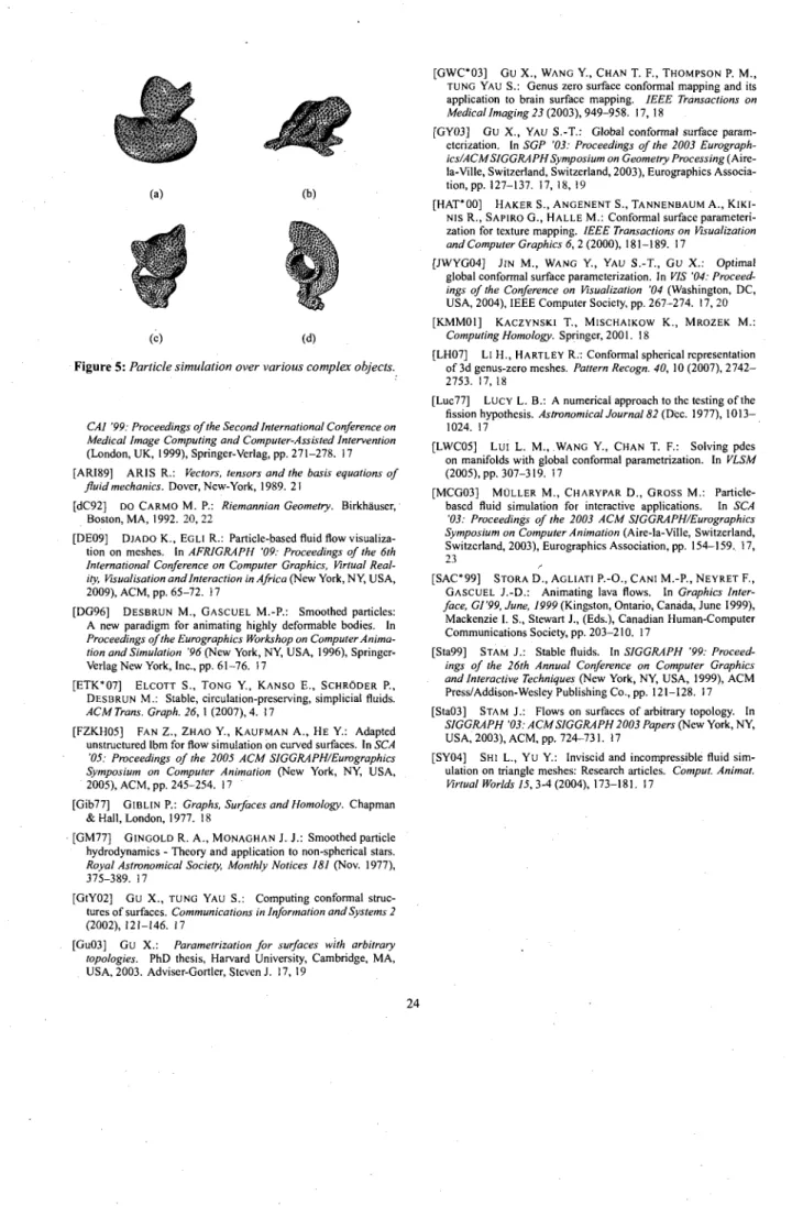
Various other examples are shown in Figure 5. External forces are added by dragging the mouse over the mesh or over the parameter domain.
/(VlnX)x ( n x V l n t y , {n)x\
B=\(V\nX)y (nxV\nX)y (n)y
\(VlnX.)z («xVlnX.)z (n)zJ
-B~lu
6. Results
The method is now applied to different situations, to confirm that simulation time is in fact independent of the mesh reso-lution, and to demonstrate free-surface flows. Various other examples will also be presented to complete the section. All results presented in this section were obtained with a 2.6GHz Intel Core 2 Quad processor.
The resolution independence is demonstrated in Table 1 where the simulation time for a single frame is displayed for every resolution of a given mesh. A torus is used as the simulation domain in this example.
Figure 4 demonstrates free-surface flows over a torus and
7. Conclusion
In this paper, we have presented a particle-based method for simulating fluid flows on the surface of an object of genus 0 or 1. The idea is to conformally map the triangle mesh to a constant curvature domain and solve the Navier-Stokes equations on the parameter domain. The uniform stretch-ing property of conformal maps ensures minimal changes to these equations. The reformulation of the advection term lets the particles follow the geodesic path without distortions caused by the parameterization.
Results show that the simulation time is independent of the resolution of the mesh, so real-time performance is achieved even with high resolution triangle mesh. The method was used to simulate free-surface flows by taking ad-vantage of the natural surface tracking that a particle-based simulation offers.
References
[AHTK99] ANGENENT S., HAKER S., TANNENBAUM A., KIKINIS R.: Conformal geometry and brain flattening. In
(c) (d)
Figure 5: Particle simulation over various complex objects.
CAI '99: Proceedings of the Second International Conference on Medical Image Computing and Computer-Assisted Intervention
(London, UK, 1999), Springer-Verlag, pp. 271-278. 17 [ARI89] ARIS R.: Vectors, tensors and the basis equations of
fluid mechanics. Dover, New-York, 1989. 21
[dC92] DO CARMO M. P.: Riemannian Geometry. Birkhauser, Boston, MA, 1992. 20,22
[DB09] DJADO K., EGLI R.: Particle-based fluid flow visualiza-tion on meshes. In AFRJGRAPH '09: Proceedings of the 6th
International Conference on Computer Graphics, Virtual Real-ity, Visualisation and Interaction in Africa (New York, NY, USA,
2009), ACM, pp. 65-72. 17
[DG96] DESBRUN M., GASCUEL M.-P.: Smoothed particles: A new paradigm for animating highly deformable bodies. In
Proceedings of the Eurographics Workshop on Computer Anima-tion and SimulaAnima-tion '96 (New York, NY, USA, 1996),
Springer-VerlagNew York, Inc., pp. 61-76. 17
[ETK*07] ELCOTT S., TONG Y., KANSO E., SCHRODER P., DESBRUN M.: Stable, circulation-preserving, simplicial fluids.
ACM Trans. Graph. 26, 1 (2007), 4. 17
[FZKH05] FAN Z., ZHAO Y , KAUFMAN A., H E Y : Adapted unstructured lbm for flow simulation on curved surfaces. In SCA
'05: Proceedings of the 2005 ACM SIGGRAPH/Eurographics Symposium on Computer Animation (New York, NY, USA,
2005), ACM, pp. 245-254. 17
[Gib77] GIBLIN P.: Graphs, Surfaces and Homology. Chapman & Hall, London, 1977. 18
[GM77] GINGOLD R. A., MONAGHAN J. J.: Smoothed particle hydrodynamics - Theory and application to non-spherical stars.
Royal Astronomical Society, Monthly Notices 181 (Nov. 1977),
375-389. 17
[GtY02] Gu X., TUNG YAU S.: Computing conformal struc-tures of surfaces. Communications in Information and Systems 2 (2002), 121-146. 17
[Gu03] Gu X.: Parametrization for surfaces with arbitrary
topologies. PhD thesis, Harvard University, Cambridge, MA,
USA, 2003. Adviser-Gortler, Steven J. 17,19
m&$
(a)
[GWC*03] Gu X., W A N G Y., C H A N T. F., T H O M P S O N P. M., TUNG YAU S.: Genus zero surface conformal mapping and its application to brain surface mapping. IEEE Transactions on
Medical Imaging 23 (2003), 949-958. 17, 18
[GY03] G u X., YAU S.-T.: Global conformal surface param-eterization. In SGP '03: Proceedings of the 2003
Eurograph-ics/ACM SIGGRAPH Symposium on Geometry Processing
(Aire-la-Ville, Switzerland, Switzerland, 2003), Eurographics Associa-tion, pp. 127-137. 17, 18, 19
[HAT*00] H A K E R S., A N G E N E N T S., TANNENBAUM A., K I K I -NIS R., SAPIRO G., HALLE M.: Conformal surface parameteri-zation for texture mapping. IEEE Transactions on Visualiparameteri-zation
and Computer Graphics 6, 2 (2000), 181-189. 17
[JWYG04] J I N M „ WANG Y., YAU S.-T., G U X.: Optimal global conformal surface parameterization. In VIS '04:
Proceed-ings of the Conference on Visualization '04 (Washington, DC,
USA, 2004), IEEE Computer Society, pp. 267-274. 17, 20 [KMM01] KACZYNSKI T., M I S C H A I K O W K., M R O Z E K M.:
Computing Homology. Springer, 2001. 18
[LH07] Li H., HARTLEY R.: Conformal spherical representation of 3d genus-zero meshes. Pattern Recogn. 40, 10 (2007), 2742-2753. 17, 18
[Luc77] L u c y L. B.: A numerical approach to the testing of the fission hypothesis. Astronomical Journal 82 (Dec. 1977), 1013— 1024. 17
[LWC05] Lui L. M., WANG Y., CHAN T. F.: Solving pdes on manifolds with global conformal parametrization. In VLSM (2005), pp. 307-319. 17
[MCG03] M U L L E R M., CHARYPAR D „ G R O S S M.: Particle-based fluid simulation for interactive applications. In SCA
'03: Proceedings of the 2003 ACM SIGGRAPH/Eurographics Symposium on Computer Animation (Aire-la-Ville, Switzerland,
Switzerland, 2003), Eurographics Association, pp. 154-159. 17, 23
[SAC*99] STORA D., AGLIATI P.-O., C A N I M.-P., N E Y R E T F., GASCUEL J.-D.: Animating lava flows. In Graphics
Inter-face, GI'99, June, 1999 (Kingston, Ontario, Canada, June 1999),
Mackenzie I. S., Stewart J., (Eds.), Canadian Human-Computer Communications Society, pp. 203-210. 17
[Sta99] STAM J.: Stable fluids. In SIGGRAPH '99:
Proceed-ings of the 26th Annual Conference on Computer Graphics and Interactive Techniques (New York, NY, USA, 1999), ACM
Press/Addison-Wesley Publishing Co., pp. 121-128. 17 [Sta03] STAM J.: Flows on surfaces of arbitrary topology. In
SIGGRAPH '03: ACM SIGGRAPH 2003 Papers (New York, NY,
US A, 2003), ACM, pp. 724-731.17
[SY04] S H I L., Y U Y.: Inviscid and incompressible fluid sim-ulation on triangle meshes: Research articles. Comput. Animal.