Record Number:
Author, Monographic: Fortin, J. P.//Villeneuve, J. P.//Benoît, J.//Blanchette, C.//Montminy, M. Proulx, H.//Moussa, R.//Bocquillon, C.
Author Role:
Title, Monographic: HYDROTEL 2.0 : user's guide Translated Title:
Reprint Status: Edition:
Author, Subsidiary: Author Role:
Place of Publication: Québec Publisher Name: INRS-Eau Date of Publication: 1990
Original Publication Date: 10 janvier 1990 Volume Identification:
Extent of Work: ix, 156 Packaging Method: pages Series Editor:
Series Editor Role:
Series Title: INRS-Eau, Rapport de recherche Series Volume ID: 286
Location/URL:
ISBN: 2-89146-295-5
Notes: Rapport annuel 1989-1990
Abstract: 25.00$
Call Number: R000286
HYDROT1:L 2.0 USER'S GUIDE.
HYDROTEL 2.0 USER'S GUIDE by Jean-Pierre FORTIN Jean-Pierre VILLENEUVE Jérôme BENOIT Claude BLANCHETfE Martin MONTMINY Hilaire PROULX Roger MOUSSA Claude BOCQUILLON Scientific Report INRS-Eau No 28b
By: Université du Québec Institut national de la recherche scientifique INRS-Eau 2700, rue Einstein C.P.7500 Sainte-Foy (Québec) G1V4C7 CANADA 10 January 1990
For: Hydrology Division Environment Canada Ottawa, Ontario K1AOE7
and
Application Division Canada Center for Remote Sensing 1547 Marivale Road Ottawa, Ontario K1AOY7
TABLE OF CONTENTS
TABLE OF CONTENTS ...•... i
LIST OF TABLES ... iv
LIST OF FlqURES ... v
PART 1 GENERAL INFORMATION ... 2
1.1 Software main characteristics and hardware requirements ... ... ... 2
1.2 Introduction ... ."... 2
1.3 Organization of the manual ... 4
1.4 Software availability and information ... 4
PART 2 THE HYDROTEL PROGRAM (2.0) ... 7
2.1 General model structure ... ... 7
2.2 Getting started ... ... 8
2.2.1 Ust of files on floppy disks ... ... ... 8
2.2.2 Installing HYDROTEL 2.0 ... 10
2.2.3 Test data and structure of data files ... 12
2.3 Using HYDROTEL (2.0) ... ... ... ... ... ... ... ... ... 25
2.3.1 Starting HYDROTEL 2.0 ... ... ... ... ... ... ... ... ... 25
2.3.2 Main menu " ... ... .... ... 25
2.3.3 Sub-menu #1.0: simulation parameters ... ... ... 26
2.3.3.1 Sub-menu #1.1: paths of files ... 27
2.3.3.2 Sub-menu #1.2: temporal parameters ... 28
2.3.3.3 Sub-menu #1.3: spatial parameters ... 30
2.3.4 ~.' Sub-menu #2.0: data input ... 31
2.3.4.1 Sub-menu #2.1: file name specification ... ... .... ... 32
2.3.4.1.1 Sub-menu #2.1.1: basin data ... ... ... ... ... 33
2.3.4.1.2 Sub-menu #2.1.2: initial settings ... ... ... ... ... 34
2.3.4.1.3 Sub-menu #2.1.3: intermediate data ... ... ... .... ... ... 35
2.3.4.2 ' Sub-menu #2.2: data format specification .... ... ... 36
2.3.4.2.1 Sub-menu #2.2.1: hydrological and meteorological data ... 37
2.3.4.2.2 Sub-menu #2.2.2: basin data ... .... ... ... ... 38
2.3.4.2.3 Sub-menu #2.2.3: initial settings ... 39
2.3.4.2.4 Sub-menu #2.2.4: intermediate data ... 40
2.3.4.3 Sub-menu #2.3: read data ... ... ... ... ... ... ... 41
2.3.4.3.1 Sub-menu #2.3.1: basin data ... .... ... ... ... .... 42
2.3.4.3.2 Sub-menu #2.3.2: initial settings ... .... ... ... .... ... 43
2.3.4.4 Sub-menu #2.4: display data ... ... .... ... 44
2.3.5 Sub-menu #3.0: sub-models . ... .... ... .... ... 45
2.3.5.1.1 2.3.5.1.2 2.3.5.1.3 2.3.5.2 2.3.5.2.1 2.3.5.1.1 2.3.5.2.1.2 , 2.3.5.3 2.3.5.3.1 2.3.5.3.1.1 2.3.5.3.1.2 2.3.5.3.1.3 2.3.5.3.1.4 2.3.5.4.2 2.3.5.4 2.3.5.4.1 2.3.5.4.1.1 2.3.5.4.1.2 2.3.5.4.1.3 2.3.5.4.1.4 2.3.5.4.1.5 ' 2.3.5.4.1.6 2.3.5.4.2 2.3.5.4.2.1 2.3.5.4.2.2 2.3.5.4.2.3 2.3.5.4.2.4 2.3.5.5 2.3.5.5.1 2.3.5.6 2.3.6 2.3.6.1 ~~,.' 2.3.6.1.1 2.3.6.1.2 2.3.6.2 2.3.6.2.1 2.3.6.2.2 2.3.6.3 2.3.6.3.1 2.3.6.3.2 2.3.6.4 2.4 2.4.1 2.4.1.1 2.4.1.2 Page
Sub-menu #3.1.1: Thiessen polygons ... ... ... ... ... 47
Sub-menu #3.1.2: weighted mean of nearest three stations .... ... 48
Sub-menu #3.1.3: arithmetic mean of nearest three stations ... ... 49
Sub-menu #3.2: snowmelt ... 50
Sub-menu #3.2.1: modified degree-day method ... ... 51
Sub-menu #3.2.1.1: parameters ... 52
Sub-menu #3.2.1.2: land-use groups ... 54
Sub-menu #3.3: evapotranspiration ... ... ... ... ... 52
Sub-menu #3.3.1: potential evapotranspiration ... 56
Sub-menu #3.3.1.1 : Thorthwaite PE ... ... 57
Sub-menu #3.3.1.2: Unacre P.E. ... 58
Sub-menu #3.3.1.3: Penman P.E. ... 59
Sub-menu #3.3.1.4: Priestley-Taylor P.E ... 61
Sub-menu #3.3.2: actual evapotranspiration ... 62
Sub-menu #3.4: vertical water budget ... ~ .... 63
Sub-menu #3.4.1: CEQUEAU (modified) ... ... ... ... 64
Sub-menu #3.4.1.1: runoff on impervious areas ... ... ... 65
Sub-menu #3.4.1.2: unsaturated zone reservoir .. ... ... 66
Sub-menu #3.4.1.3: saturated zone reservoir ... ... ... ... 67
Sub-menu #3.4.1.4: lakes and marshes ... ... 68
Sub-menu #3.4.1.5: initiallevels in reservoirs ... 69
Sub-menu #3.4.1.6: land-use groups ... 71
Sub-menu #3.4.2: BV3C ... 72
Sub-menu #3.4.2.1: soil and land-use files ... 73
Sub-menu #3.4.2.2: parameters characterizing layers ... 74
Sub-menu #3.4.2.3: general parameters ... 75
Sub-menu #3.4.2.4: land-use groups ... 76
Sub-menu #3.5: surface and sub-surface runoff .. ... ... 77
Sub-menu #3.5.1: land-use groups ... 78
Sub-menu #3.6: channel routing ... ... 79
Sub-menu #4.0: data output ... ... ... ... ... 80
Sub-menu #4.1: file name specification ... ... ... ... ... 80
Sub-menu #4.1.1: intermediate results ... 81
Sub-menu #4.1.2: final settings ... ... ... ... 82
Sub-menu #4.2: data format specification ... ... ... ... 83
Sub-menu #4.2.1: intermediate results ... 84
Sub-menu #4.2.2: final settings ... 85
Sub-menu #4.3: save data ... 85
Sub-menu #4.3.1: intermediate results ... 87
Sub-menu #4.3.2: final settings .. ... ... 88
Sub-menu #4.4: display data ... ... 89
Calibration of model parameters and initialization of state variables ... 95
Calibration of model parameters ... ... 95
Control criteria ... 95
Pre-calibration sensitivity analysis ... 95 ii
Page
2.4.1.3 Subjective calibration ... ... ... ... 96
2.4.2 Initialization of state variables ... 96
2.4.2.1 Vertical water profile ... : ... 97
2.4.2.1.1 CEQUEAU (modified) ... 97
2.4.2.1.2 BV3C ... 98
2.4.2.2 Water in transit ... 99
2.4.2.2.1 First simulation on a new basin .... ... ... 99
2.4.2.2.2 Ali further simulations on a basin for which initialization files do exist ... '" ... 101
2.5 Integration of user's developed sub-models ... 101
PART 3 MAIN SIMULATION EQUATIONS AND FLOW CHARTS ... 103
3.1 Introduction ... ... 103
3.2 Spatial distribution of precipitation ... 103
3.2.1 Thiessen polygons ... 103
3.2.2 Weighted mean of nearest three stations ... 104
3.2.3 Arithmetic mean of nearest three stations ... 104
3.3 Snow cover simulation and melting ... 104
3.3.1 Transformation of rainfall into snowfall ... 104
3.3.2 Simulation of snowpack transformation and melt ... 105
3.3.3 Input variables ... 106
3.4 Evapotranspiration ... 108
3.4.1 Potential evapotranspiration ... 108
3.4.1.1 Thornthwaite potential evapotranspiration ... 108
3.4.1.1.1 The equation ... 1 08 3.4.1.1.2 Input data ... 109
3.4.1.2 3.4.1.2.1 .::q, Unacre potential evapotranspiration ... ... 109
The equation ... 109
3.4.1.2.2 Input data ... 111
3.4.1.3 Monteith - Penman potential evapotranspiration ... 112
3.4.1.3.1 The equation .. '" ... 112
3.4.1.3.2 Input data ... 115
3.4.1.4 ' Priestley-Taylor potential evapotranspiration ... 116
3.4.1.4.1 The equation ... 116
3.4.1.4.2 Input data ... 117
3.5 Vertical water budget ... 117
3.5.1 CEQUEAU (modified) ... '" ... 118
3.5.1.1 Description ofthe function ... 118
3.5.1.2 Input data ... 120
3.5.2 BV3C ... 122
3.5.2.1 Description of the function ... 122
3.5.2.2 3.5.2.3 3.6 3.6.1 3.6.2 3.7 3.7.1 3.7.1.1 3.7.1.2 3.7.2 3.7.2.1 3.7.2.2 3.8 3.9 Page Input variables ... '" ... 131
Interaction of the root system with the soillayers ... 132
Surface and sub-surface runoff ... 134
Kinematic wave equations ... 135
Input data '" ... 136
Channel routing ... ... 137
Modified kinematic wave equations ... 138
Theory ... 138
Input data ... ... ... 140
Diffuse wave equation ... 140
Theory ... 140
Input data ... 143
land-use classification ... 143
Soil types and hydraulic characteristics ... 146
REFERENCES ... : ... 150
Table 2.1 Table 3.1
LIST OF TABLES
Page Julian days ... ... ... 29 Soil hydraulic properties classified by soil texture ... 148
LIST OF FIGURES
Figure 1.1 Integrated analysis of physical, remotely sensed and meteorological data for steamflow simulation and
forecasting by PHYSITEL, IMATEL and HYDROTEL ... ... ... ... 3
Figure 2.1, Spatial structure ofthe model .. ... ... ... 7
Figure 2.2 Streamflow and climatological stations on the Eaton basin ... 12
Figure 2.3 Main menu .... ... ... ... ... .... ... ... 26
Figure 2.4 Sub-menu #1.0: simulation parameters ... ... ... ... 26
Figure 2.5 Sub-menu #1.1: paths to files ... 27
Figure 2.6 Sub-menu #1.2: temporal parameters ... ... ... ... 28
Figure 2.7 Sub-menu #1.3: spatial parameters ... 30
Figure 2.8, Sub-menu #2.0: data input ... 31
Figure 2.9 Sub-menu #2.1: file name specification ... 32
Figure 2.1D Sub-menu #2.1.1: basin data .. ... ... ... ... ... 33
Figure 2.11 Sub-menu #2.1.2: initial settings .... ... ... ... 34
Figure 2.12 Sub-menu #2.1.3: intermediate data ... 35
Figure 2.13 Sub-menu #2.2: data format specification ... ... ... 36
~" Figure 2.14 Sub-menu #2.2.1: hydrological and meteorological data... 37
Figure 2.15 Sub-menu #2.2.2: basin data ... ... 38
Figure 2'.16 Sub-menu #2.2.3: initial settings .... ... ... 39
Figure 2.17 Sub-menu #2.2.4: intermediate data ... ... 40
Figure 2.18 Sub-menu #2.3: read data ... ... ... ... ... 41
Figure 2.19 Sub-menu #2.3.1: basin data ... 42
Figure 2.20 Sub-menu #2.3.2: initial settings ... ... ... 43
Page
Figure 2.21 Sub-menu #2.4: display data ... 44
Figure 2.22 Sub-menu #3.0: sub-models ... ... ... ... .... ... 45
Figure 2.23 Sub-menu #3.1: interpolation of precipitation .... ... ... ... 46
Figure 2.24 \ Sub-menu #3.1.1: Thiessen polygons ... ... ... ... 47
Figure 2.25 Sub-menu #3.1.2: weighted mean of nearest three stations ... 48
Figure 2.26 Sub-menu #3.1.3: arithmetic mean of nearest three stations .. ... ... 49
Figure 2.27 Sub-menu #3.2: snowmelt ... ... ... 50
Figure 2.28 Sub-menu #3.2.1: modified degree-day method ... 51
Figure 2.29 Sub-menu #3.2.1.1: parameters ... 52
Figure 2.30 Sub-menu #3.2.1.2: land-use groups ... 54
Figure 2.31, Sub-menu #3.3: evapotranspiration .. ... 55
Figure 2.32 Sub-menu #3.3.1 : potential evapotranspiration ... ... 56
Figure 2.33 Sub-menu #3.3.1.1: Thorthwaite PE ... ... ... 57
Figure 2.34 Sub-menu #3.3.1.2: Unacre P.E. ... 58
Figure 2.35 Sub-menu #3.3.1.3: Pen man P.E. ... 59
Figure 2.36 Sub-menu #3.3.1.4: Priestley-Taylor P.E. ... 61
'-",-Figure 2.37 Sub-menu #3.3.2: actual evapotranspiration ... 62
Figure 2.38 Sub-menu #3.4: vertical water budget ... 63
Figure 2.39 Sub-menu #3.4.1: input data for CEQUEAU ... 64
Figure 2.40 Sub-menu #3.4.1.1: runoff on impervious areas ... 65
Figure 2.41 Sub-menu #3.4.1.2: unsaturated zone reservoir ... 66
Figure 2.42 Sub-menu #3.4.1.3: saturated zone reservoir ... ... ... ... 67
Figure 2.43 Sub-menu #3.4.1.4: lakes and marshes ... ... ... ... ... ... 68
Figure 2.44 Sub-menu #3.4.1.5: initiallevels in reservoirs . ... ... ... ... 69 vii
Page
Figure 2.45 Sub-menu #3.4.1.6: land-use groups ... 71
Figure 2.46 Sub-menu #3.4.2: BV3C ... 72
Figure 2.47 Sub-menu #3.4.2.1: soil and land-use files ... 73
Figure 2.48 , Sub-menu #3.4.2.2: parameters characterizing layers ... 74
Figure 2.49 Sub-menu #3.4.2.3: general parameters ... 75
Figure 2.50 Sub-menu #3.4.2.4: land-use groups ... 76
Figure 2.51 Sub-menu #3.5: surface and sub-surface runoff ... 77
Figure 2.52 land-use groups for surface and sub-surface runoff .... ... 78
Figure 2.53 Sub-menu #3.6: channel routing .. '" ... ... ... ... 79
Figure 2.54 Sub-menu #4.0: data output ... ... ... ... ... ... 80
Figure 2.55 Sub-menu #4.1: file name specification ... -.. ... ... ... 81
Figure 2.56 Sub-menu #4.1.1: intermediate results ... ... ... ... 81
Figure 2.57 Sub-menu #4.1.2: final settings . ... ... ... 82
Figure 2.58 Sub-menu #4.2: data format specification ... 83
Figure 2.59 Sub-menu #4.2.1: intermediate results ... ... 84
Figure 2.60 Sub-menu #4.2.2: final settings ... 85
'-':",.-Figure 2.61 Sub-menu #4.3: save data ... ... ... 86
Figure 2.62 Available water from rain and/or melt ... 86
Figure 2~63 Sub-menu #4.3.1: intermediate results ... 87
Figure 2.64 Sub-menu #4.3.2: final settings . .... ... 88
Figure 2.65 Sub-menu #4.4: display data ... ... ... ... 89
Figure 2.66 Tabular informations on variables related to squares ... ... 90
Figure 2.67 Tabular informations on variables related to reaches ... 91 Figure 2.68 Tabular informations on variables related to CEQUEAU water budget. 91
Page
Figure
2.69
Tabular informations on variables related to BV3C water budget ...92
Figure 2.70 Streamflow hydrograph ... 93
Figure 3.1 Vertical water budget adapted from the CeaUEAU model ... 119
Figure
3.2 ,
Vertical water budget in BV3C ...122
Figure
3.3
Figure 3.4 Figure3.5
Figure3.6
Variation of the matrix potential with9 ... 125
Interaction ofthe root system with the soillayers ... 133
Surface and sub-surface runoff and channel flow ... 135
Finite difference scheme for the solution of the diffusive wave equation ...
142
PART 1
HYDROTEL 2.0 - 2
PART 1 GENERAL INFORMATION
1.1
Software main characteristics and hardware requirements
Name: HYDROTEL 2.0 Objective: Programming languages: Type of microcomputer: Memory requirements: Written by: Developed by: "::",-1.2
Introduction
Simulation of streamflows using ground and remotely sensed data.
IBM PC/XT or AT and compatibles with a mathematical co-processor.
640K.
Jérôme Benoît, Claude Blanchette and Martin Montminy. Jean-Pierre Fortin, Jean-Pierre Villeneuve, Jérôme Benoît, Claude Blanchette, Martin Montminy and Hilaire Proulx at INRS-Eau, Quebec, Canada.
Claude Bocquillon and Roger Moussa, LHM, USTL, Montpellier, France.
Considering, as others (peck et aL, 1981; Rango, 1985), that there was a need for the development of hydrological models compatible with remotely sensed data, INRS-Eau began such a development a few years ago. Work was undertaken on various aspects of hydrological modelling, namely: type of simulation for surface and sub-surface runoff as weil as for channel routing, determination of basin topography from a digital elevation model (DEM), display and analysis of images on microcomputers, land-use determination for hydrological purposes, integration of weather radar and station data ...
HYDROTEL 2.0 - 3
At the beginning, the model was seen as one pragram allowing determination of basin topography fram DEM, land-use determination from the analysis of remotely sensed images and hydrological simulation and forecasting. As seen in figure 1.1, it was thought later on that the large number of tasks would be handled more easily by three interrelated software packages instead of one. The HYDROTEL package will be devoted to hydralogical simulation and forecasting. As such, it will receive input data in the proper format from PHYSITEL (topography) and IMATEL (land-use and daily operational data
(surface temperature, albedo, ...
».
IMA~ SPOT ERS-J. REnOle".':' HVDROMETEO. ARCHIVES ~~l
, METEOSAT PEDOLOGV TOPOGRAPHV <DEH) Figure 1.1 LAND-USEr:l
1 PHVSICAL~
.... : _D_A_T_A_-m . . . ._ - _, 1 :oth~ 1 ;sysLI L _ _ _ • 1 FILES FOR SPECIFI BASINS PHVSICAL DATA ANALVSIS ; STREAMFLOW SIMULATION AND FORECAST ( PRECIPITATION. SHOW COVER, SOIL MOISTURE •••• )Integrated analysis of physical, remotely sensed and meteoralogical data for steamflow simulation and forecasting by PHYSITEL, IMATEL and HYDROTEl.
As seen by INRS-Eau the status of the current HYDROTEL version (V 2.0) is the following:
HYDROTEL 2.0 structure has been conceived and pragrammed to answer users needs and facilitate the graduai addition of ail wanted options to a fully "à la carte" model, as weil as the input and output of G.I.S. and time dependent data;
HYDROTEL 2.0 - 4
HYDROTEL2.0 should
be
regarded as only a step in the development of the model originally conceived.HYDROTEL 2.0, allows the testing of any of the sub-models without having to include ail parts of the water cycle (ail sub-models) in a particular run, provided the
appropr~ate input files are furnished.
HYDROTEL 2.0 is presented with better data displays.
HYDROTEL 2.0 stores simulation parameters for the next simulation so that the users does not have to go through the whole input process each time he wants to proceed to a new simulation. Only the parameters he wants to change need a new input.
1.3 Organization of the manu al
Part "ONE" of the manual contents general information on HYDROTEL 2.0.
ln part "lWO", the user is first told how to install the computer program. Information on the data set furnished with the program is then given. This data set is made available to the user to allow him to get acquainted with the model. Information on how to start the program is next given. This is followed by a detailed information, window by window, on the simulation choices, and input data.
A description of the main simulation methods available with HYDROTEL 2.0 is finally given in part ''THREE'', together with hints on how to select values for model parameters.
1.4 Software availability and information
The current version (2.0) of HYDROTEL is available only to Environment Canada and CCRS personnel participating in the testing of that version, to help defining the options that should be available in HYDROTEL (2.nn).
Agreements with other agencies is also possible. For informations, contact:
~.-Prof. Jean-Pierre Fortin INRS-Eau
2800, rue Einstein, bureau 105 Québec (Québec) G1X4N8 CANADA Téléphone: (418) 654-2591 Telex: Fax: 051-31623 (418) 654-2600 HYDROTEL 2.0 - 5
PART 2
HYDROTEL 2.0 - 7
PART 2 THE HYDROTEL PROGRAM (2.0) 2.1 General model structure
Before gettiog into detailed informations on how to use the HYDROTEL model, it should be known first that it is a distributed model. This means that variables like rainfall, snowCQver, snowmelt, evapotranspiration, soil moisture and ground water are spatially discretized, as are also surface and subsurface runoff and channel routing (figure 2.1). It is thus possible to keep track of what happens anywhere in a given basin at any time step. " '2.
'"
1 2 3 " 5 12 13,.
Il ~_ ~ 2 3 4 5 6 7 8 9 10 11 12Figure 2.1 Spatial structure of the modal.
o
®
©
2 3 .. 5 6 7 e 9 10 Il 12 @ 1 2 3 '.. 5 6 7 e 9 10 Il 12®
TRANSFfRT FUNCTfONAnother main characteristic of HYDROTEL is that it is divided into modules, each offering a number of options. These modules are:
- INPUT (interactive input of ail necessary data to run the model);
- PHYSIOGRAPHY (management and storage of topography and land use data);
- PRECIPITATION (divided into 2 sub-modules: interpolation of precipitations and snowcover and snowmelt simulation);
HYDROTEL 2.0 - 8
- EVAPOTRANSPIRATION (estimation of potential evapotranspiration);
- HYDROLOGY (divided into 3 sub-modules: vertical water budget, surface and subsurface runoff and channel routing);
- OUTPUT (screen display, files saving and retrieving, hard print); - MAIN (management of ail tasks).
A third characteristic of HYDROTEL is the possibility for the user to incorporate its own simulation options to those already available in the modal. This characteristic should be very interesting for specifie applications. This means that, if a user has developed a program for the simulation of a particular part of the hydrologie cycle, it could be possible for him to integrate it in the HYDROTEL program as a new user's defined option.
2.2 Getting starled
This section gives ail necessary informations to install the program on your microcomputer. A data set is also furnished with the model to help the user to get acquainted with
it.
2.2.1 List of files on floppy disks
HYDROTEL 1.1 is sent on three 1.2 M floppy disks. Content:
Disk #1: program disk. CONFIG.SYS
KERNEL.SYS HYDROTEL.EXE HYDROTEL.ENM HYDROTEL.MAK
\OBJ (compiled modules)
\BASINS (Clifton data for the year 1973). Disk #2: Display and printer drivers disk. Adage/Lexidata PG90 Model 30
AT&T 6300/6310 - 640 x 400 Monochrome AT&T 6300/6310 - 640 x 400 Coler
Compaq Portable III Display DGIS High Performance Displays Hercules InColor Display
Hercules Monochrome Graphies Adapter High Resolution EGA Displays
IBM 8S14/a 1024 x 768 Display IBM 8S14/a 640 x 480 Display
IBM Color Graphies Adapter - High Res. Mono. IBM Coler Graphies Adapter - Med. Res. Coler IBM Enhanced Graphies Adaptor - 4 modes IBM Personal System/2 - Mode 11
IBM Personal System/2 - Mode 12 IBM Personal System/2 - Mode 13 Toshiba 3100 Lap Top Display HP laser jet EPSON LQ series EPSON *X series HYDROTEL 2.0 - 9 ADAGE30.SYS CGI6300B.SYS CGI6300C.SYS COMPAQ3.SYS CGIDGIS.SYS HERCINCO.SYS HERCBW.SYS HIRESEGA.SYS IBMAFH.SYS IBMAFL.SYS IBMBW.SYS IBMCO.SYS IBMEGA.SYS IBMVGA 11.SYS IBMVGA 12.SYS IBMVGA13.SYS T3100.SYS LASERJET.SYS EPSONLQ.SYS EPSONX.SYS
Disk #3: Data disk.
Results obtained with default values for: C:\ CLIFTON.TEM CLlFJON.PRE CLIFTON.FON CLIFTON.ETP CLIFTON.PRO CLIFTON.RUI CLIFTON.DEB \BASINS\ CLIFTON.ALT CLlFTOt-;J.CLA CLIFTON.CLU CLlFTON.lCR CLlFTON.lRO CLIFTON.MSK CLIFTON.NDS CLIFTON.ORI CLIFTON.PCP CLIFTON.PTE CLIFTON.SOL CLIFTON.STN CLIFTON.TRO CLIFTON.TSO ALBEDO.VY HAU VEG.VY
-PRO RAC.VY -INF FOL.VY -M7020885.73 M7020885.74 M7022280.73 M7022280.74 2.2.2 lnstalling HYDROTEL 2.0 M7022306.73 M7022306.74 M7027802.73 M7023312.73 M7023312.74 M7027372.73 M7027372. 74 M7027520.73 M7027520. 74 M7024263.73 M7024263.74 HYDROTEL 2.0 - 10 M7024624.73 M7024624. 74 M7027802. 74 M7028124.73 M7028124.74 M7028906.73 M7028906.74 H0030242.73 H0030242. 74
The AUTOEXEC.BAT and CONFIG.SYS files on your system should first be modified to run HYDROTEL 1.1:
- modifications to AUTOEXEC. BAT file add: SET KERNEL=c:\HYDROTEL
- modifications to CONFIG.SYS file add: FILES =30
DEVICE =c:\dir\name.SYS
where: "dira is the directory where the display driver is. "name.SYS" is the code name of the display driver. DEVICE=C:\dir\name.SYS
where: "dir" is the directory where the printer driver is
"name.SYS" is the code name of the printer driver. DEVICE = \GSSCG1. SYS
Note: the previous command may be modified to: DEVICE = \ GSSCGI.SYS/T
HYDROTEL 2.0 - 11
ln that case, only the essential parts of the GSS program are loaded when . booting the computer, saving memory space for other programs run on the computer. It is then necessary to copy DRIVERS.EXE in c:\HYDROTEL. Otherwise, this is not necessary.
When the AUTOEXEC.BAT and CONFIG.SYS files are mOdified, one may praceed with the other files. Since paths to files are asked for in the menu, the user may copy the files in any directory or subdirectory.
The following procedure is suggested, but is not mandatory. It is assumed that the micracomputer has a hard disk and that the user is already on C:
1. create a new directory (or subdirectory) HYDROTEL, using the MS-DOS command MD;'
2. change trom the current directory (or subdirectory) to the new directory HYDROTEL, using the MS-DOS command CD;
3. copy ail model files fram disk #1 to that subdirectory; 4. make a subdirectory BASINS;
HYDROTEL 2.0 - 12
5. change to that subdirectory;
6. copyall data files from disk #1 (1973) or disk #3, to that subdirectory. You should now be ready to start the program.
2.2.3 Test data and structure of data files
ln order to familiarize the user with HYDROTEL 2.0, a data set is included with the program. At the same time, it should be looked at as an example, for the preparation of other data sets.
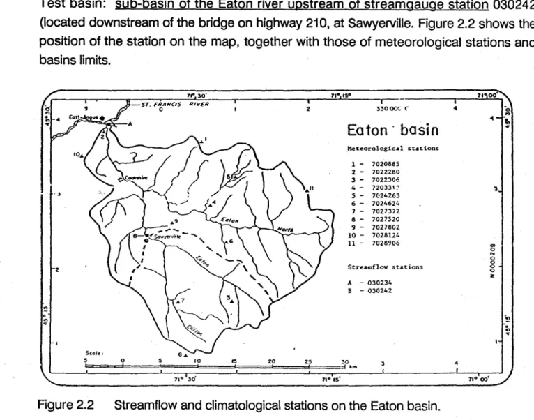
Test basin: sub-basin of the Eaton river upstream of streamgauge station 030242 (Iocated downstream of the bridge on highway 210, at Sawyerville. Figure 2.2 shows the position of the station on the map, together with those of meteorological stations and basins Iimits. ., o ., '" 2 Sca'~: 5 0 fe:t ' 7" 30' ST. FRANCIS RivER o '0 15
.
20 . 2 25 : 33000c ("Eafon' basin
Heteorological stations 1 - 1020885 2 - 1022280 3 - 1022306 4 - 120331 ~ 5 - 1('24263 6 - 1024624 1 - 1027372 8 - 1027520 9 - 1027602 10 - 1028124 11 - 7028906 Streamflov stations A - 030234 B - 030242 30 1 "tnFigure 2.2 Streamflow and climatological stations on the Eaton basin.
3 en o N o o o o z o '" ...
HYDROTEL 2.0 - 13
Are included in the data set: topographie data:
- File names and content:
- Clifton.ALT: mean altitude of each square (m);
- Clifton.ORI: aspect of each square to eight points of the compass, identified 1 to 8 counterclockwise from East (= 1);
- Clifton.PTE: slope of each square (m/m); - Clifton.MSK: basin mask;
- Clifton.NDS: information on reach ends (identification number, UTM coordinates (m), altitude (m) and channel width (m);
- Clifton.TRO: information on reaches (identification numbers for lower and higher ends (in that order), Manning's roughness coefficient). - File structure for *.ALT,*.ORI,*.PTE,*.MSK:
- line #1: file type: 1;
- li ne #2: number of lines, number of colums;
- line #3: UTM coordinates (Easting, Northing) of upper left corner, grid size (m); - line #4: title or comment identifying the file;
- line #5 to 4
+
(Ii X co): data (separated by blanks). - File structure for *.NDS:- line #1: file type: 1;
- line #2: number of reach ends;
- line #3: title or comment identifying the file;
- line #4 to (3
+
number of reach ends): identification number, Easting, orthing, altitude (m), channel width (m).HYDROTEL 2.0 - 14
- File structure for *.TRO: - line #1: file type: 1;
- line #2: number of reaches (= number of reach ends - 1); - line #3: title or comment identifying the file;
- line,#4 to (3
+
number of reaches): identification numbers for downstream and upstream ends, Manning's roughness coefficient.land-use data:
- File names and content:
- Clifton.CL.A: spatial distribution of land-use classes;
- Clifton.CLU: time invariant characteristics of land-use classes;
- Albedo.YV: albedo values of each land-use c1ass as a function of time for year "YVU
;
- Hau veg.YV: height of each land-use class as a function of time, for year "VY"; - Pro_rac.YV: depth reached by the root system, of each land-use class, as a
function of time, for year "VY";
- Inf fol.YV: leaf-area index of each land-use c1ass, as a function of time, for year "yyu.
- File structure for *.CL.A: - li ne #1: file type: 1;
- line #2: number of lines, number of cOlumns, number of classes; - line #3: EAST, NORTH, class codes, TOTAL;
- 'line #4 to 3
+
(Ii x co): UTM coordinates (Easting, Northing) of upper left corner, number of pixels belonging to each class, total number of pixels.- suggested class identification and codes: - bare fields: "champ";
HYDROTEL 2.0 - 15
- crops and pasture 2: "paill"; - extracting areas: "gravi";
- forested areas 1 (coniferous): "resin"; - forested areas 2 (deciduous): ''feuil'';
- highways and other impervious areas: "route"; - ~urface waters 1: "eau1";
- surface waters 2: "eau2"; - urban areas: "urb" (not in use);
- waste lands and bushes: ufrich" and "coupe"; - wet lands and marshes: "MAR" (not in use). - File structure for *.CLU:
- line #1: file type: 5;
- line #2: number of land-use classes, number of characteristics for eaeh land-use class;
- line #3: - line #4:
title or comment identifying the file; Nom _ COT COT CO ZS ZV ZP;
(Une #4 is considered as a comment. It is there only ta help in the identification of the values below. The user can change the wording, but not the arder).
- line #5 ta 4
+
number of land-use classes: maximum fraction CO(!) of the relative water content at field capacity useful for land-use elass 1,,<. (LUC1), maximum depth at which vegetation of LUC 1 can pomp water at a rate equal ta Co (1), depth reached by the roots when the root system is fully developed at the surface, maximum depth of the root system at maturity.
(Remember that ZV < ZP-ZS. The arder in which land-use classes are listed is not important, but the code names must be the same as that given in *.CLA).
- File structure for Albedo.VY, hau _ veg.VY, Pro _rae.VY, Ind _foI.VY: - line #1: file type: 2;
- line #2: - line #3: - line #4:
HYDROTEL 2.0 - 16
number of land-use classes, number of days (N of D) for which values are available, year;
title or comment identifying the file;
Month, Day, land-use class (LUC) code (1), LUC code (2), ... , LUC code (#LUC).
- line,#5 to 4
+
N of D: actual values for month, day and LUC (same order as decided in line #4).Soil data:
(fhe order in line #4 is not important, but he code names must be the same as that given in *.CLA. The extension "YY" should be changed to that of the actual year .eg. "73").
- File names and content:
- Clifton.SOL: hydraulic characteristics of soil types;
- Clifton.TSO: spatial distribution of soil types in the watershed. - File structure for *.SOL:
- line #1: - line #2: - line #3: - Iinè#4:
file type:
3;
number of soil types, number of characteristics for each sail type; title of comment identifying the file;
Name Thetas Thetacc Thetaph KS PSIS Lambda Alpha
{Une #4 is considered as a comment. It is there only ta help in the identification of the values below. The user can change the wording, but not the arder.
fine #5 ta 4
+
number of soil types: code name, water content at saturation (m3m-3), water content at field capacity (m3m-3), water content at the permanent wilting point (m3m-3), hydraulic conductivity (mh-1),matrix potential at 8s (m), pore size distribution, coefficient in eq.
HYDROTEL 2.0 - 17
- File structure for *.TSO: - line #1: file type: 4;
- line #2: number of lines, number of columns;
- line #3: UTM coordinates (Easting, Northing), spatial resolution (m); - line #4: title or comment identitying the file.
- fine #5 to 4
+
(number of line -1):code (0,0) - - - code (0, ncol-1)
1
code (nlig -1,0) - - - code (nlig-1, ncol-1) where the code values correspond to entries in file *.SOL. A code value of "0" corresponds to the first soil type, a code value of "1"
corresponds to the second soil type in *.SOL and so on. Streamflow and meteorological data available for use in the simulation: - List of meteorological stations:
- file name: Clifton.STM: - file structure:
- line #1: file type: 1;
- li ne #2: number of meteorological stations; - line #3: title or comment identifying the file;
- line #4 to (3
+
number of stations) identification number, longitude (degrees and minutes), latitude (degrees and minutes), altitude (m);- List of streamflow stations: - file name: Clifton.STH - file structure:
- line #1 : file type: 1;
HYDROTEL 2.0 - 18
- line #3: title or comment identifying the file;
- line #4 to (3
+
number of stations): identification number, longitude (degrees and minutes), latitude (degrees and minutes), altitude (m);INRS data formats
- streamflow data (ms) at streamgauge station 030242 for 1973 and 1974, beginning on the 1 st of January of each year;
- file name: H030242.VY (H station identification.year): - file structure:
- line #1: station identification, year, number of valid values;
line #2 to 32: 366 daily streamflows. Missing data (including February 29): -1000.
- meteorological data (maximum daily air temperature, minimum daily air temperature, rainfall, snowfall), for 1973 and 1974, beginning on the 1st of January of each year, at the following stations:
- 7020885 Bury;
- 7022280 East-Angus; - 7022306 Eaton 2nd Branch; - 7023312 Island Brook; - 7024263 Lawrence; - 7024624 Maple Leaf East; - 7027372 St-Isidore d'Auckland; - 7027520 St-Malo d'Auckland; - 7027802 Sawyerville Nord; - 7028124 Sherbrooke A; - 7028906 West Ditton.
HYDROTEL 2.0 -19
- file name: M7020885.VY (M station identification.year): - file structure:
- line #1: station identification, year, numbers (4) of valid data for maximum temperature, minimum temperature, rain and snow respectively. latitude in degrees and minutes, longitude in degrees and minutes, altitude (m), station identification;
- line #2 to 17: 366 maximum temperature (OC); - line #18 to 33: 366 minimum temperature (OC); - line #34 to 49: 366 rainfall values (10-1mm);
- Une #50 to 65: 366 snowfall values (10-1cm). - missing data:
- temperatures: -99; - rainfall or snowfall: -1.
Environment Canada data formats
- Format for streamflow data (from Environment Canada card format 79-041 (daily discharges)
Daily discharges for each month are stored on three 80 colums lines. General format for each line:
Colum's
1 code for type of data and units. Q-daily discharges in cubic metres per second 2-8: station number, e.g. 08AA023
9-11: year, e.g. "968" for 1968 12-13: month, e.g. "b?" for July
14: code for time interval
1: daily figures from day 1 ta day 20 2: daily figures tram day 11 ta day 20 3: daily figures from day 21 ta day 31 15-80: ten or eleven 6 - character data fields Comments:
- Each data field has six positions.
HYDROTEL 2.0 - 20
The first five positions contain daily discharge data, right justified with a decimal point if necessary; the sixth position contains a symbol.
- Whenever data are missing the value "-9999" is entered in positions 1-5 and position 6 cantains a blank.
- The first line contains 10 days fram day 1 ta 10; colums 75-78 are not used; the number of days in the month, e.g. "30" for November, is typed in colums 79-80. - The secand line cantains 10 days from day 11 ta 20; colums 75-80 are not used. - The third line cantains 11 days fram day 21 ta 31 ; the figure "-1111" is written in the
appropriate field for days that do not apply ta the months e.g. 30 and 31 for February 1968, and position 6 contains a blank.
- Format for meteoralogical data (fram Format documentation for the digital archive of canadian climatological data).
- Oaily values: Oaily values are archived as 232 character long monthly records. - File structure:
Colum(s)
1-7: station identification (alphanumeric) 8-10: year, e.g. "973" for 1973 (numeric)
11-12: month, e.g. 01 = JAN. etc (numeric) 13-15: elements number (numeric)
16-232: 31 7-character groups structured as follows: 1st character: sign "_" = negative
"0" = positive 2nd to 6th character: data value (numeric) 7th character: Flag (alphanumeric)
- File content (depending on element number):
The following elements are read and used in HYDROTEL 2.0 - maximum temperature: 001 (.1°c)
- minimum temperature: 002 (.1°c) - Total precipitation: 012 (.1mm) - Hourly values:
Hourly values are archived as 185 character long daily records. - File structure:
Colum(s)
1-7: station identification (alphanumeric) 8-10: year, e.g. "973" for 1973 (numeric) 11-12: month, e.g. 01 = JAN. etc (numeric) 13-14: day (numeric)
'15-17: element number (numeric)
18-185: 24 7-character groups structured as follows: 1 st character: sign "-" = negative
"0" = positive 2nd to 6th character: data value (numeric) 7th character: Flag (alphanumeric)
- File content (depending on element number):
The following elements are read and used in HYDROTEL 2.0 - wind: 076 (km h-1)
- relative hymidity: 080 (%)
- bright sunshine: 133 (.1 h)
- global solar radiation: 061 (.001 = MJjm2)
Intermediate results
- Format for values on squares:
The following variables are concerned: - temperatures (*.TPX and *.TPN) - rain (*.PRE)
- snowOlelt (*.FON)
- potential evapotranspiration (*.ETP) - outflow (*.PRO)
- runoff (*.RUI) - File structure:
- line #1 : file type: 1 (integer)
HYDROTEL 2.0 - 22
- line #2: number of lines, number of colums in the grid (integers)
- li ne #3: UTM coordinates (Easting, Northing) of upper left corner (long integers), grid size (m) (integer)
- li ne #4: simulation period: - starting year (integer) - starting day (integer) - duration in days (integer)
- line #5: title or comment identifying the file
- line #6 to end of file: groups of daily values, one for each day of the simulation, structured as follows:
- First line in the group: number of days since the beginning of the simulation
HYDROTEL 2.0 - 23
- Ali other lines in the group: (Ii X co) values recorded by lines ta facilitate display.
- Format for streamflow values in reaches. The foJlowing file is concerned:
Streamflows (*.DEB) - File structure:
- line #1: file type: 1 (integer)
- line #2: number of reaches (integer) - line #3: simulation period
- starting year (integer) - starting day Onteger) - duration in days (integer)
- li ne #4: title or comment identifying the file
- line #5 ta end of file: groups of daily values, one for each day ta of the simulation, structured as follows:
- First line in the group: number of days since the beginning of the simulation
("0" for the first day). - Ali other lines in the group:
-- reach identification number (integer) - lateral input (real)
- streamflow at downstream mode (real) Initial settings of state variables
- Initial settings for the vertical water budget (file *.PIS). - File structure:
- line #1: file type: 1 (integer)
HYDROTEL 2.0 - 24
- line #3: UTM coordinates (Easting, Northing) of upper left corner (long integers), grid size (ml Onteger)
- line #4: title or comment identifying the file
- line #5 to end of file: three groups of (Ii X co) values corresponding respectively to water levels in the soil (1), ground water (2) and lakes and marshes
(3) reservoirs in the CEQUEAU vertical water budget option. Initial settings for surface and sub-surface runoff (file *.RIS)
- File structure:
- line #1: file type: 1 Onteger)
- line #2: number of Unes, number of colums in the grid (integers)
- line #3: UTM coordinates (Easting, Northing) of upper left corner (long integers), grid size (ml Onteger)
- line #4: title or comment identifying the file - line #5 to end of file: (Ii X co) runoff values (real) Initial settings for streamflows in reaches (file *.CIS) - File structure:
- line #1: file type: 1 (integer)
- lins #2: number of reaches (integer) - line #3: title or comment identifying the file - line #4 to end of file:
For line #i corresponding to reach j
- index number for downstream end (different fram identification number) - index number for upstream end
- downstream flow (real) - upstream f10w (real) - lateral inflow (real)
HYDROTEL 2.0 - 68
- Outflow coefficient: type the outflow coefficient.
- Fraction of PET taken in saturated zone: type the nominal fraction of potential evapotranspiration taken from the saturated zone.
- Reference level for fraction of PET (mm): type the reference level (in millimeters) for which the effective fraction of evapotranspiration taken fram the saturated zone reservoir is that given above.
When this is done, leave the sub-menu by pressing "F10" (accept and save the new values) or "ESC" (no change to previously stored values).
2.3.5.4.1.4 Sub-menu #3.4.1.4: lakes and marshes (figure 2.43)
MAIN MENU
1._ Simulation parameters;
2.
3.- SUB-MODELS
4.-5.- 1. Interpolation of precipitations;
6. 2. Snowmelt;
O. - 3. - r - - - . ~4.- VERTICAL WATER BUDGET
5. -6. l.
0.- 2.- CEQUEAU (MODIFIED)
"-- 3.
4.-
1. Runoff on impervious areas;
O.
2.- Unsaturated zone reservoir;
~
3'=jSaturated zone
re~ervoir;4. [1
LAKES AND MARSHES ,F=============ïI
5.
6. Threshold for outflow (mm) ... 250
O. Outflow coefficient ... 2.5e-002
'
-4F10:Acceptl
IEsc:QuitF
HYDROTEL 2.0 - 25
2.3 Using HYDROTEL (2.0)
2.3.1 Starting HYDROTEL 2.0
Your files should now be in the proper directories or sub-directories, including your own basin files or the test files.
If you are not there, first come back (change) to c:\HYDROTEL.
Now, type "HYDROTEL" and the main menu will appear on the screen.
If
"/T"
has been added to the command "DEVICE=\GSSCGI,SYS" in the CONFIG.SYS file, when in c:\HYDROTEL, type "DRIVERS" before typing "HYDROTEL". Typing "DRIVERS/R" when going out of HYDROTEL 2.0 will free memory space for other programs.It should be mentioned at this stage that a tree structure has been developed for menus. The menus are written in a logical order so that even an unfamiliar user should normally be able to go through ail steps in the initialization process easily.
2.3.2 Main menu
The main menu contains 7 options (figure 2.3). To choose an option, first go to that option using the arrows on the keyboard. Then, push the "ENTER" key. The sub-menu needed to define that option will appear.
When the last simulation is finished, you can go out of HYDROTEL by choosing the "End of simulation" option and pressing "ENTER".
From the main menu, it is possible to go to "DOS" to use DOS commands and come back to HYDROTEL. This may be useful to edit files, for instance.
MAIN MENU
1. Simulation parameters;
2.-
Data input;
3.-
Sub-models;
4.-
Data Output;
5.-
Run;
6.-
DOS shell;
0.-End of simulation.
Figure 2.3 Main menu.
2.3.3 Sub-menu #1.0: simulation parameters
HYDROTEL 2.0 - 26
Sub-menu #1 (figure 2.4) contains 3 options. Each of these options leads you to a new sub-menu in which simulation parameters are defined. You can return to the previous (main) menu (by selecting option "0" followed by the "ENTER" key).
MAIN MENU
1. SIMULATION PARAMETERS
2.-3.
1.Path to fil es;
4.- 2.-
Temporal parameters;
5.- 3.-
Spatial parameters;
6.- 0.-
Return to previous menu.
O.-L---~
HYDROTEL 2.0 - 27
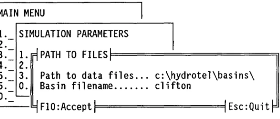
2.3.3.1 Sub-menu #1.1: paths to files
Informations on paths to files used by HYDROTEL have to be given here (figure 2.5):
MAIN MENU
11. SIMULATION PARAMETERS
t=:
1.~PATH
TO FILES:F==============il
4. 2.
5.- 3.
Path to data files .. .
6.-
o.
Basin filename ... .
c:\hydrotel\basins\
cl
ifton
0 . - - J
-
jFlO:Acceptl=l ==========IIEsc:Quit
Figure 2.5 Sub-menu #1.1: paths to files.
- path to data files: it has been suggested in section 2.2 to group data files in a particular sub-directory. The path to files in that sub-directory should be given here; - basin filename: this is the name under which ail data files for a particular basin will be
identified. As an example, the general name for ail data in the set furnished with the program is "CLIFTON". Particular files are identified by "CLIFTON.***", with the stars corresponding to letters and/or numbers identifying the specifie file.
At any time in that sub-menu you can quit the initialization process by pushing "ESC". The paths and basin name appearing on the screen remains in effect. No change is made to the previously stored name.
Normally, once the information is given you want to confirm or accept il. Press "F10". The paths to files are stored for later use by the program and return to the previous sub-menu #1.0 is done automatically.
HYDROTEL 2.0 - 28
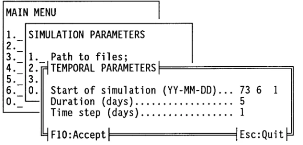
2.3.3.2 Sub-menu #1.2: temporal parameters
Back to sub-menu #1.0, go to the next option "Temporal parameters" and press "ENTER" to get sub-menu #1.2 (figure 2.6):
- start of simulation
rrv
MM DO): year (Iast two digits), month and day of the first day of the simulation;- duration (NN): the number of consecutive days in the simulation;
- time step (days): only one time step is allowed with HYOROTEL 2.0: 1 day.
Ali those values are entered by going to the proper line with the arrows on the keyboard and typing the appropriate values. When this is done, accept (and save) the values by pressing F10.
If you want to leave the menu without change, press "ESC".
MAIN MENU
11. SIMULATION PARAMETERS
2.-3. -
1.Path to fil es;
4.
=
2.
-ri
TEMPORAL PARAMETERS
:1===========iI
5. 3.
6.-
O. St art of simulation (YY-MM-DD) ... 73
6
1
O.-~
Duration (days) ... 5
-
Time step (days) ... 1
~F10:Acceptl
IEsc:Quit
TABLE 2.1 Julian days.
DAY Jan. Feb. March April May June Ju1y 1 1 32 60 91 121 152 182 2 2 33 61 92 122 153 183 3 3 34 62 93 123 154 184 4 4 35 63 94 124 155 185 5 5 36 64 95 125 156 186 6 6 37 65 96 126 157 187 7 7 38 66 97 127 158 188 ~ 8 39 67 98 128 159 189 9 9 40 68 99 129 160 190 10 10 41 69 100 130 161 191 11 11 42 70 101 131 162 192 12 12 43 71 102 132 163 193 13 13 44 72 103 133 164 194 14 14 45 73 104 134 165 195 15 15 46 74 105 135 166 196 16 16 47 75 106 136 167 197 17 17 48 76 107 137 168 198 18 18 49 77 108 138 169 199 19 19 50 78 109 139 170 200 20 20 51 79 110 140 171 201 21 21 52 80 111 141 172 202 22 22 53 81 112 142 173 203 23 23 54 82 113 143 174 204 24 24 55 83 114 144 175 205 25 25 56 84 115 145 176 206 26 26 57 85 116 146 177 207 27 27 58 86 117 147 178 208 28 28 59 87 118 148 179 209 29 29 ie 88 119 149 180 210 30 30 89 120 150 181 211 31 31 90 151 212
,'c For leap years, add 1 ta julian day after February 28th.
Aug. Sept. Oct. 213 244 274 214 245 275 215 246 276 216 247 277 217 248 278 218 249 279 219 250 280 220 251 281 221 252 282 222 253 283 223 254 284 224 255 285 225 256 286 226 257 287 227 258 288 228 259 289 229 260 290 230 261 291 231 262 292 232 263 293 233 264 294 234 265 295 235 266 296 236 267 297 237 268 298 238 269 299 239 270 300 240 271 301 241 272 302 242 273 303 243 304 Nov. Dec. 305 335 306 336 307 337 308 338 309 339 310 340 311 341 312 342 313 343 314 344 315 345 316 346 317 347 318 348 319 349 320 350 321 351 322 352 323 353 324 354 325 355 326 356 327 357 328 358 329 359 330 360 331 361 332 362 333 363 334 364 365 DAY 1 2 3 4 5 6 7 8 9 10 11 12 13 14 15 16 17 18 19 20 21 22 23 24 25 26 27 28 29 30 31 :c
-<
o :0o
-1 m r l'V o , 1\) <0HYDROTEL 2.0 - 30
2.3.3.3 Sub-menu #1.3: spatial parameters
Back to sub-menu #1.0, go to the next option "Spatial parameters" and press "ENTER" to get sub-menu #1.3 (figure 2.7):
- upper left corner (UTM): enter the upper left corner of the rectangular grid containing the basin, in UTM coordinates. Note: this will be change in later versions of HYDROTEL to use other coordinate systems more suitable to large basins;
- lower right corner (UTM): enter the lower right corner of the rectangular grid containing the basin, in UTM coordinates;
- resolution (m): enter grid size in meters. No more th an 40 squares are allowed in either direction, N-S or E-W, leading to a 40 x 40 matrix, of which only 900 squares can be within the basin. This number is much larger th an needed.
When this is done, accept (and save) the values by pressing "F10".
MAIN MENU
11. SIMULATION PARAMETERS
2.
-3.
1.Path to fil es;
4.= 2.=J Temporal
parameter~;5. _ 3.
1SPATIAL PARAMETERS
,1==============i1
6. O.
O. - ~ UlM zone... 19
Upper left corner (UTM) .... 295000
5026000
Lower right corner (UTM) ... 316000
5007000
Resolution (m) ... 1000
9
FlO :Accept
1
1
Esc: Quit
~Figure 2.7 Sub-menu # 1.3: spatial parameters.
HYDROTEL 2.0 - 31
Back ta sub-menu #1.0 (figure 2.4), go ta "Return ta previous menu" and press "ENTER" ta go back ta the "main menu".
2.3.4 Sub-menu #2.0: data input
Sub-menu #2.0 (figure 2.8) leads the user ta windows in which he will be able ta provide the informations on input data needed for the simulation.
MAIN MENU
l.
2.- DATA INPUT
3.-4._ 1._ File name specification;
5. 2. Data format specification;
6.- 3.- Read data;
0.- 4.- Display data;
~
0.- Return to previous menu.
HYDROTEL 2.0 - 32
2.3.4.1 Sub-menu #2.1: file name specification
Sub-menu #2.1 leads to three sub-menus in which the necessary file informations can be given for basin data, initial settings and intermediate data.
MAIN MENU
1.
12.- DATA INPUT
3.-4. 1. FILE NAME SPECIFICATION
5. 2.
6.- 3. 1. Basin data;
0.- 4.- 2.- Initial settings;
~0.- 3.- Intermediate data;
~
O.
Return ta previaus menu.
HYDROTEL 2.0 - 33
2.3.4.1.1 Sub-menu #2.1.1: basin data
Appropriate file names corresponding to ail types of basin data Iisted in sub-menu 2.1.1 (figure 2.10) should appear in that window.
MAIN MENU
1.
12.-
DATA INPUT
~:=
1._
FI~
NAME SPECfFICATION
15._ 2._
[1BASIN
DATAI~============== 6. 3. 1.0.- 4.- 2. Meteo station id ... clifton.stm
~0.-
3. Streamflows station id ... clifton.sth
~O.
Basin mask ... clifton.msk
'-- Altitude ... cl ifton.alt
Aspect ... clifton.ori
Slope ... clifton.pte
Land-use classes ... clifton.cla
Reach ends ... clifton.nds
Reaches ... clifton.tro
~FIO:Acceptl
IEsc:QuitF
HYDROTEL 2.0 - 34
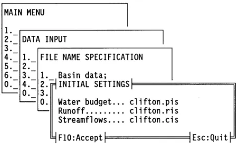
2.3.4.1.2 Sub-menu #2.1.2: initial settings
Initial values can be given to variables representing the hydrologie state of the basin at the beginning of the simulation. File names are given here. Otherwise, the initial settings default to zero ("Q") for surface and subsurface runoff and channel routing. In the case of the vertical budget, initial values can be also given in sub-menu 3.4.1.5. Informations on how to determine these initial values are given in the section on "initialization of state variables" at the end of Part 2.
MAIN MENU
1.
12.- DATA INPUT
3.-4. 1. FILE NAME SPECIFICATION
5. 2.
6.- 3.- 1. Basin data;
0.= 4.=
2.-~INITIAL SETTINGS:F===========ïI
'-- O. 3.
~
O. Water budget ... clifton.pis
~
Runoff ... clifton.ris
Streamflows .... clifton.cis
~
F10:Accept 1=1 ========11 Esc:Quit
HYDROTEL 2.0 - 35
2.3.4.1.3 Sub-menu #2.1.3: intermediate data
Names of the files containing intermediate data are given here (figure 2.12).
MAIN MENU
1. 1
2.- DATA INPUT
3.-4.
1.
FILE NAME SPECIFICATION
5.-
2.-6.- 3.
1.Basin data;
0.= 4.= 2.=Jlnitial settings;1
'-- 0._ 3.
lINTERMEDIATE DATA11===========;J
-
O.
--- Max. temp ... clifton.tpn
Min. temp ... clifton.tpx
Rain ... clifton.pre
melt ... clifton.fon
Pot. evap ... clifton.etp
Outflow ... clifton.pro
Runoff ... cl i fton. rui
Streamflows .... clifton.deb
9
FlO:Acceptl=l ======lIEsc:Quit
HYDROTEL 2.0 - 36
2.3.4.2 Sub-menu #2.2: data format specification
Data formats to read the various files are chosen in the menus accessed from menu 2.2 (figure 2.13). Further format options wiU be provided in later versions. For HYDROTEL 1.1 aU files are ASCII text files.
MAIN MENU
1.
-2.
-DATA INPUT
3.
-4.
- 1.-5. 2.
- -DATA FORMAT SPECIFICATION
6. 3.
0.-
4.
-1._ Meteo
&
hydro data;
' - - -
O.
2.
Basin data;
-
-3.
Initial settings;
-
-4.
-Intermediate data;
O.
-Return to previous menu.
HYDROTEL 2.0 - 37
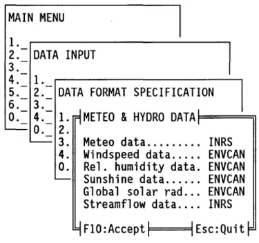
2.3.4.2.1 Sub-menu #2.2.1: hydrological and meteorological data
Environment Canada or INRS data formats can be chosen, using the "space" bar.
MAIN MENU
1.2.- DATA INPUT
3. -4. 1.5.- 2.- DATA FORMAT SPECIFICATION
6.-3.- ~ 1
0.-
4.=
1.ln
METEO
&HYDRO DATA,I=======iI
'--- o.
2 •...=
3. Meteo data ... INRS
4. Windspeed data ... ENVCAN
o.
Rel. humidity data. ENVCAN
~
Sunshine data ... ENVCAN
Global solar rad ... ENVCAN
Streamflow data .... INRS
YFIO:Acceptl
IEsc:Quitr
HYDROTEL 2.0 - 38
2.3.4.2.2 Sub-menu #2.2.2: basin data.
Only INRS ASCII text file format is available with HYDROTEL 1.1 (figure 2.15).
MAIN MENU
1.
2.-
DATA INPUT
3.-4.- 1.
5.- 2.-
DATA FORMAT SPECIFICATION
6.-
3.-0.= 4.=
l'_jMeteo
&
hY1ro data;
'-- 0._ 2. rlBASIN DATA,I==========
'-- 3.
4. Meteo station id ... INRS
O. Streamflows station id ... INRS
~
Basin mask ... INRS
Altitude ... INRS
Aspect. . . ..
1NRS
Slope ... INRS
Land-use classes ... INRS
Reach ends ... INRS
Reaches ... INRS
4
FIO:Accept
11======91
Esc:Quit
HYDROTEL 2.0 - 39
2.3.4.2.3 Sub-menu #2.2.3: initial settings
Only INRS ASCII text file format is available with HYDROTEL 2.0 (figure 2.16).
MAIN MENU
1.
2.- DATA INPUT
3.-4. - 1.
5.- 2.- DATA FORMAT SPECIFICATION
6.-
3.-0.- 4.- 1. Meteo
&
hydro data;
~
0.- 2.- Basin data;
-=
3.-, INITIAL SETTINGS
:1======iI
4.
O. Water budget .... INRS
-
Runoff... INRS
Streamflows ... INRS
, Fla
:Accept
H
Esc: Qui t
1= Figure 2.16 Sub-menu #2.2.3: initial settings.HYDROTEL 2.0 - 40
2.3.4.2.4 Sub-menu #2.2.4: intermediate data
Only INRS ASCII text file format is available with HYDROTEL 2.0 (figure 2.17).
MAIN MENU
1.
2.- DATA INPUT
3.-4.- 1.
5.- 2.- DATA FORMAT SPECIFICATION
6.-
3.-0.- 4.-
1.Meteo
&
hydro data;
~
0.- 2.- Basin data;
~3'=JInitial settings;1
4.
Il
INTERMEDIATE DATA 1
1======;'1O.
~Temperatures ... INRS
Rain ... INRS
melt ... INRS
Pot. evap ... INRS
Outflow ... INRS
Runoff ... INRS
Streamflows .... INRS
~
FlO :Accept
H
Esc: Qui t
~
HYDROTEL 2.0 - 41
2.3.4.3 Sub-menu #2.3: read data
With HYDROTEL 2.0, sub-menu 2.3 (figure 2.18) is optional. Basin data will be read automatically, but not initial settings of the state variables. This sub-menu will be used in later versions to permit data input from more th an one file for each variable. This will allow, for instance integration of two groups of files on contiguous basins, if not already done by PHYSITEL.
MAIN MENU
1.
-2.
-DATA INPUT
3.
-4.
- 1. -Fil e name specification;
5. 2.
--6. 3.
- -READ DATA
O. 4.
- -' - - -O.
1.Basin data;
--2.
Initial settings;
'-O. - Return to previous menu.
HYDROTEL 2.0 - 42
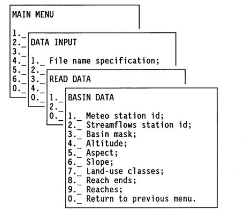
2.3.4.3.1 Sub-menu #2.3.1: basin data
With HYDROTEL 2.0, sub-menu 2.3.1 (figure 2.19) is optional. Data will be read automatically.
MAIN MENU
1.
-2.
-DATA INPUT
3.
-4.
- 1. -Fil e name specification;
5.
2.
6.
--3.
--READ DATA
1o.
-4.
-' - - -o.
1.BASIN DATA
- -' - - -2.
-o.
- 1. -Meteo station id;
' - - -
2.
Streamflows station id;
-3.
-Basin mask;
4.
Altitude;
5.= Aspect;
6._ Slope;
7.
-Land-use classes;
8.
-Reach ends;
9.
-Reaches;
o.
-Return to previous menu.
HYDROTEL 2.0 - 43
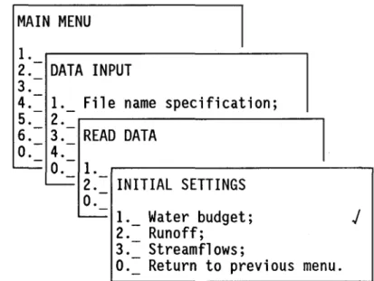
2.3.4.3.2 Sub-menu #2.3.2: initial settings
With HYDROTEL 2.0, sub-menu 2.3.2 (figure 2.20) is optional. If the user wants to initialize the state variables with values computed in a previous run, he must select the corresponding options. Otherwise, runoff and streamflow values will default to zero and water budget variables will have to be read at sub-menu 3.4.1.5.
MAIN MENU
l.
-2.
-DATA INPUT
3.
-4.
- l. -Fil e name specification;
5.
-2.
-6.
-3.
-READ DATA
o.
-4.
-' - - - -o.
l. - -' - - - -2.
INITIAL SETTINGS
-o.
-1._ Water budget;
J
-2.
-Runoff;
3.
Streamflows;
o.
- Return to previous menu.
HYDROTEL 2.0 - 44
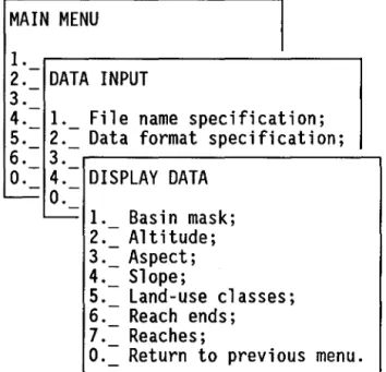
2.3.4.4 Sub-menu #2.4: display data
If one wants to have a visual representation of files containing basin data, he can select any of the options in sub-menu 2.4 (figure 2.21). The selected variable will be displayed on the screen, together with an appropriate legend.
MAIN MENU
1.
2.-
DATA INPUT
3.-4.-
1. File name specification;
5. 2. Data format specification;
6. 3.
0.- 4.- DISPLAY DATA
---=
0.----=
1.Basin mask;
2.-Altitude;
3.-
Aspect;
4. Slope;
5.= Land-use classes;
6._ Reach ends;
7._ Reaches;
0._ Return to previous menu.
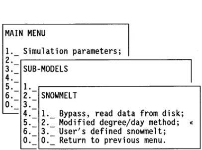
2.3.5 Sub-menu #3.0: sub-models
MAIN MENU
1. Simulation parameters;
2.-,---.
3.-
SUB-MODELS
4.-5.-
1. Interpolation of precipitations;
6.- 2.-
Snowmelt;
0.- 3.-
Evapotranspiration;
~4.-
Vertical water budget;
5.-
Surface and sub-surface runoff;
6.-
Channel routing;
0.-
Return to previous menu.
Figure 2.22 Sub-menu #3.0: sub-models.
HYDROTEL 2.0 - 45
Ali options (figure 2.22) can be selected by moving to each of those options and pressing "ENTER". After typing ail necessary data, in the sub-menus corresponding to those options return to the "main menu" by selecting option "0" and pressing "ENTER". It is possible to Olby pass" any of the submodels. In HYDROTEL 2.0, intermediate data corresponding to the output from that sub-model has then to be read.
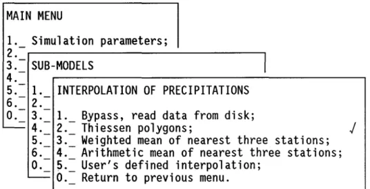
2.3.5.1 Sub-menu #3.1: interpolation of precipitation See section 3.2 for more informations.
MAIN MENU
1. Simulation parameters;
2.-
13.-
SUB-MODElS
4.-5. 1. INTERPOLATION OF PRECIPITATIONS
6. 2.0.- 3.-
1. Bypass, read data from disk;
~
4.- 2.-
Thiessen polygons;
j
5.- 3.-
Weighted mean of nearest three stations;
6.- 4.-
Arithmetic mean of nearest three stations;
0.- 5.-
User's defined interpolation;
~
0.-
Return to previous menu.
Figure 2.23 Sub-menu #3.1: interpolation of precipitation.
HYDROTEL 2.0 - 46
Five options are available for the interpolation of precipitations (figure 2.23). Select one of those and press "ENTER". After typing the input values, return to "sub-menu 3.0" by selecting option "0" and pressing "ENTER".
Option 1 allows the user to bypass interpolation of precipitation by reading instead precipitation matrices obtained from a previous run or elsewhere, for example from weather radar or satellite data. Precipitation values are read from the file specified in sub-menu 2.1.3 (intermediate data). It will be also possible for the user to write its own interpolation submodel, following the instructions given in this user's guide.
2.3.5.1.1 Sub-menu #3.1.1: Thiessen polygons (figure 2.24)
MAIN MENU
1. Simulation parameters;
2.-
13.- SUB-MODELS
4.-
~---~5. 1. INTERPOLATION OF PRECIPITATIONS
6.- 2.
0.-
3.-
1. Bypass, read data from disk;
~4.- 2.- Thiessen polygons;
HYDROTEL 2.0 - 47
5.= 3.=
Wei hted mean of nearrst three stations;
6._ 4._
Ar THIESSEN POLYGONS,I===========
o.
5.Us
~
0.- Re Precipitation vert. grad. (%/100m) ...
o.
Temperature lapse rate (C/I00m) ...
o.
4
FlO:AcceptFI
=========~IEsc:Quit
Figure 2.24 Sub-menu #3.1.1: Thiessen polygons.- Precipitation: vertical gradient (%/100 m): type the main vertical gradient of precipitations, in % per 100 meters. Type "0", if you consider that the vertical distribution of stations can take care of the gradient.
- Temperature: lapse rate (OC/100 m): type the temperature lapse rate in degrees Celcius per 100 meters. Type "0", if you consider that the vertical distribution of stations can take care of the lapse rate.
When this is done, leave the sub-menu by pressing "F10" (accept and save the new values) or "ESC" (no change to previously stored values).