Temporal evolution of low flow regimes in Canadian rivers.

Temporal evolution of low flow regimes

in Canadian rivers

Temporal evolution of low flow regimes in Canadian rivers

Par

. 1 * 1 2 3

M.N. Khahq , , T.B.M.J. Ouarda, P. Gachon ,L. Sushama

INSERC/Hydro-Quebec Statistical Hydrology Chair, Canada Research Chair on the Estimation of Hydrological Variables, INRS-ETE, University of Quebec, 490 de la Couronne, Quebec City, Quebec G1K 9A9, Canada

Tel: 418-654-3842, Fax: 418-654-2600, Email: nkhaliq@gmail.com

2 Atmospheric Science and Technology Directorate, Adaptation and Impacts Research Division, Environment Canada, Montreal, Quebec, Canada

30uranos Consortium on Regional Climatology and Adaptation to Climate Change, 550 Sherbrooke Street West, West Tower, 19th Floor, Montreal, Quebec H3A 1B9, Canada

Rapport de recherche N° R-986

ABSTRACT

This study investigates temporal evolution of 1-, 7-, 15- and 30-day annual and seasonal low· flow regimes of pristine river basins, included in the Canadian reference hydrometric basin network (RHBN), for three time frames: 1974-2003, 1964-2003 and 1954-2003. For the analysis, the RHBN stations are classified into three categories, which correspond to stations where annual low flows occur in winter only, summer only and both summer and winter seasons, respectively. Unlike in previous studies for the RHBN, such classification is essential to better understand and interpret the identified trends in low flow regimes in the RHBN. Nonparametric trend detection and bootstrap resampling approaches are used for the assessment of at-site temporal trends under the assumption of short-term persistence (STP). The results of the study demonstrate that previously suggested pre-whitening and trend free pre-pre-whitening approaches are inadequate in capturing the STP structure of low flow regimes compared to a bootstrap based approach. The analyses of 10 relatively longer records reveal that trends in low flow regimes exhibit fluctuating behavior and hence their temporal and spatial interpretations appear to be sensitive to the time frame chosen for the analysis. Furthermore, under the assumption of long-term persistence (LTP), which is a possible explanation for the fluctuating behavior of trends, many of the significant trends in low flow regimes, noted under the assumption of STP, become non-significant and their field significance also disappears. Therefore, correct identification of STP or LTP in time series of low flow regimes is very important as it has serious implications for the detection and interpretation of trends.

Keywords: Bootstrap resampling; Canada; dimate change; long-term persistence; low flows; nonparametric methods; RHBN; short-term persistence; trends.

1. INTRODUCTION

It is documented in the third assessment report of the Intergovernmental Panel on Climate Change (IPCC) [2001] that the global average surface temperature has increased by 0.6 ± 0.2 oC over the 20th century. Recently released summary of the fourth assessment report of the IPCC [2007] indicates that the global average surface temperature will increase by 1.8 to 4.0 oC by the year 2100 compared to current climate, with maximum changes being projected for the high latitude regions. Since climate is the most important driver of the hydrological cycle, the rise in temperature could cause changes in the pattern of occurrences of extreme hydrologie events (i.e., floods and droughts) and increases in their frequency and severity could pose serious challenges for sustainable management of water resources in different parts of the world, as water resources could be one of the most vulnerable to climate change. Our understanding of the climate system and magnitude of future climate change impacts is hindered by uncertainties in climate models and complex hydrological responses of catchments to climatic changes. Therefore, observational evidence plays a crucial role in addressing these uncertainties and achieving a fuller reconciliation between model-based scenarios and ground truth.

River flows represent an integrated response to various climatic inputs to a catchment and are known to be sensitive to changes in precipitation and evapotranspiration, which could occur as a result of climate change. Hence, there had been a number of studies on the identification and interpretation of temporal changes in river flow regimes in different parts of the world. Examples are Chiew and McMahon [1993], Letfenmaier et al. [1994], Lins and Slack [1999], Douglas et al. [2000], Zhang et al. [2001], Hisdal et al. [2001], Robson [2002], Burn and Hag Elnur [2002], Yue et al. [2003], Xiong and Shenglian [2004], Lindstrom and

Bergstrom [2004], Kundzewicz et al. [2005], Hannaford and Marsh [2006], among others; the objectives of these studies were the identification of temporal changes in hydrological time series through parametric, non-parametric and Bayesian approaches. Recently, Kundzewicz and Robson [2004] presented a review of the methodology and provided general guidance for the identification of hydrological trends. They recommended the use of good quality adequate baseline data in combination with a good methodology, i.e. the use of distribution-free testing and resampling methods, for reliable change detection in time series ofhydrological records.

The studies by Westmacott and Burn [1997], Gan [1998], Yulianti and Burn [1998], Déry and Wood [2005] and Rood et al. [2005] analyzed Canadian streamflow records for detecting changes at regionallbasin scales. Zhang et al. [2001] and Yue et al. [2003] focused on detecting changes at country-wide scale by analyzing streamflows from the reference hydrometric basin network (RHBN). The RHBN is a set of pristine river basins, which are minimally affected by human activities such as deforestation, urbanization, reservoirs, water abstractions, etc. None of the above studies fully explored the temporal behaviors of annual and seasonal low flows of various durations at country-wide scale using the RHBN. Therefore, the primary objective of this study is to examine the temporal trends in annual and seasonal key low flow indicators (i.e., 1-, 7-, 15- and 30-day low flows) at the country-wide scale using the RHBN. Investigation of the seasonallow flow indicators is important because occurrences of low flows in the RHBN reveal strong seasonal tendencies and therefore the analysis of only annual low flow indicators would not be adequate. The selected low flow indicators are important for water resources planning and management since severe reductions in these indicators can adversely affect riparian ecology, water quality and water availability. Individual values of these indicators represent severity of hydrological droughts experienced

in a year (or season) and have been generally used for designing safe water abstractions and waste load allocations in order to protect river water quality and aquatic ecosystems.

In low flow hydrology, it is usual to consider a representative annual or seasonallow flow index such as the annual minimum average discharge for a fixed duration [e.g., Gustard et al., 1992; Zaidman et al., 2003]; often 1-day, 7-day (most widely used) or 30-day durations are used [Smakhtin, 2003]. Flows below a suitably selected threshold have also been used to define hydrological droughts as periods during which the streamflow is below the selected threshold [e.g., Zelenhasié and Salvai, 1987; Tallaksen et al., 1997]. This paper only deals with the fixed duration low flows.

In this study, nonparametric and resampling techniques are employed for the identification of temporal trends in low flow regimes. The choice of nonparametric techniques is based on the fact that they are weIl suited in situations where minimal distributional assumptions are required to be made and where censored data and missing data problems are often encountered [Kundzewicz and Robson, 2000, 2004], as is the case with hydrological records. The resampling approaches provide altemate robust methods for assessing the significance of the observed test statistics on one hand and offer plausible means to address the issues of auto correlations in the time series being tested on the other hand. The auto correlation structure of the time series, being tested, is known to affect the accuracy of nonparametric trend investigation tests [e.g., von Storch, 1995]. These approaches are based on the assumption that the observations of hydrological variables are independent and identically distributed or possess short-term persistence (STP). On the contrary, long-term persistence (LTP) has been noted in time series of hydroc1imatological variables by some investigators, e.g. Montanari et al. [1996], Pelletier [1997], Syroka and Toumi [2001], Cohn

and Lins [2005], Koutsoyiannis [2006], Koutsoyiannis and Montanari [2007]. According to Koutsoyiannis [2003], Cohn and Lins [2005] and Koutsoyiannis and Montanari [2007], the presence of LTP has serious implications for the investigation of trends. For example, the assumption of STP can cause overestimation of significant trends if L TP is the correct working hypothesis. Therefore, it is important to consider the presence/absence of LTP in low flow regimes and its effect on the estimated trends. Similar to the effect of auto correlations on the outcome of the trend investigation test, the presence of positive cross correlation within a stream gauging network inflates the possibility of rejecting the null hypothesis of no field significance of estimated trends [Douglas et al., 2000]. For assessing the field significance of estimated trends (i.e., to control the rate of false detections), the False Discovery Rate (FDR) approach of Benjamini and Hochberg [1995] is used. The False Discovery Rate approach is recently recommended by Wilks [2006] for field significance analysis.

This paper is organized as follows. Description of the streamflow data used in the study is given in section 2. Necessary but concise description ofthe chosen statistical methods used for investigating temporal behavior of low flow regimes is presented in section 3. AIso, an appealing procedure adopted for obtaining seasonal low flows is described in section 3. Results along with main conclusions of the analyses are presented in section 4, followed by discussion in section 5.

2. DATA

The river basins of RHBN are characterized by either pristine or stable hydrological conditions. The streamflow data at all RHBN stations are acquired following a set of consistent, national standard procedures. Originally, the RHBN consisted of 249 hydrometric

stations, including continuous streamflow, seasonal streamflow and continuous lake level stations [Brimley et al., 1999; Harvey et al., 1999]. Over the years, the RHBN has evolved and currently this network consists of 229 hydrometric stations (Environment Canada, 2006, personal communication). Of the 229 hydrometric stations, 201 stations are used in the present analyses; the left out stations were either lake level stations or stations which did not have year-round continuous streamflow records. The location of these 201 stations is shown in Figure 1. The density of RHBN stations is not uniform over Canada and most of the stations are concentrated in southem Canada, south of 60oN, with certain provinces having limited spatial coverage. Basin sizes for the network of 201 stations range from 3.9 km2 to 145,000 km2. About 9% of the basins are less than 115 km2 and about the same percent is greater than 25,000 km2 while 50% ofthe basins are less than and equal to 1400 km2.

The streamflow data for the network of201 stations is obtained from the Water Survey of Canada's HYDAT data archive (http://www.wsc.ec.gc.ca/hydat/H20). At the time of writing this paper, streamflow records are available till the end of 2003 for the majority of stations except for stations located in the province of Quebec. For the Quebec stations, complete streamflow records are available till the end of 2000 and therefore the analysis for those stations is performed using data till the year 2000. The network of 201 stations consists of 8590 station years with about 78% of stations having more than or equal to 30 years of record. The minimum length of useful year-round continuous record, without missing values, is 7 years, while the maximum is 93 years. Average record length is about 43 years.

Temporal evolutions of annual and seasonal 1-, 7-, 15- and 30-day low flows are studied in detail for three time frames in order to address the uncertainty of the temporal change signal to the length of historical record. The three time frames studied are: (1)

1974-- - -

-2003, (2) 1964--2003, and (3) 1954-2003. Thus, for each n-day low flow the length of time series is either 30, 40 or 50 years. In order for a station to be included in the analysis, a maximum of 3 missing year criterion for each time frame is used. Hence, the number of stations used for each time frame is different: 156 for the 30-year period, 102 for the 40-year period and 49 for the 50-year period. The RHBN stations withTelatively longer records are used to investigate long-term behavior of seasonal n-day low flows. These stations are found in southem parts of Canada only, i.e. southem parts of Alberta, Ontario and Quebec and Atlantic provinces.

3. METHODOLOGY

3.1. Seasonal partitioning of low flows

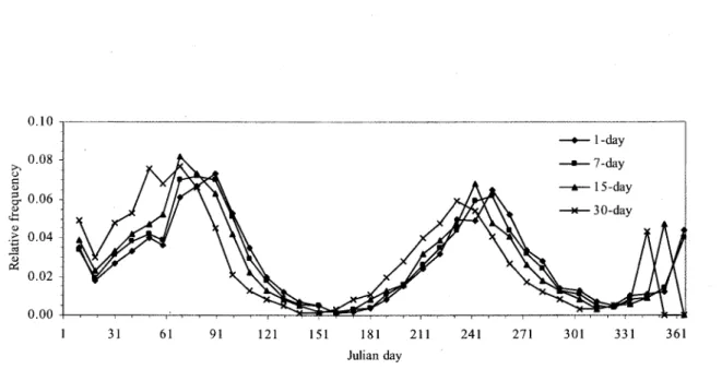
In sorne of the previous studies, e.g. Whalen and Woo [1987] for the historical streamflow records and Sushama et al. [2006] for the Canadian regional climate model simulated flows, it has been established that low flows exhibit a seasonal behavior in Canadian streams, i.e. the low flow conditions occur because of two different mechanisms. Firstly, the low flows occur as a result of storage depletion following below freezing temperatures during the winter season. Secondly, the low flows occur as a result of lack of precipitation and increased evaporation due to higher temperatures during the summer season. For the seasonal partitioning of low flow regimes, starting dates of occurrence of 1-, 7-, 15-and 30-day annual low flows are obtained from 201 RHBN stations 15-and the resulting frequency distributions of these dates are shown in Figure 2. It is quite obvious from this figure that the occurrences of annual low flows show a seasonal behavior. Therefore, annual low flows can be classified into summer low flows and winter low flows. Since it is difficult

to define exactly the date which differentiates between winter and summer low flow seasons, it is assumed that summer and winter low flows fall within the 'June to November' and 'December to May' periods, respectively. The percent age of station years during which (winter, summer) low flows were recorded are (58.8%, 41.2%), (59.7%, 40.3%), (60.4%, 39.6%) and (60.5%,39.5%) for 1-, 7-, 15- and 30-day durations, respective1y. This winter and summer seasonal partitioning of low flow regimes is based on the results presented in Figure 2. Detailed information on various other methods of seasonality analysis for river flow regimes can be found in the work of Ouarda et al. [2006].

In order to appropriately study the seasonal nature of low flow regimes, it is useful to divide the RHBN stations into three categories, i.e. CATI-stations with winter low flows only, CAT2-stations with summer low flows only, and CAT3-stations with low flows occurring in bothwinter and summer seasons. The choice of the low flow duration has a little influence on the division of stations into various categories because the number of stations which experience winter only, summer only and mixed low flows vary slightly with respect to the chosen n-day low flow duration. For the present analyses, the division of stations, shown in Figure 1, based on the seasonality of annual 7-day low flows is assumed adequate. Out of 201 RHBN stations, the number of stations for CATI, CAT2 and CAT3 are 60,14 and 127, respective1y. Majority of the CATI and CAT3 stations are found respectively above and be10w the 500

N. The CAT2 stations are small in number and are found only in southwestem British Columbia and Nova Scotia, with one station in southeastem Ontario. The seasonal behavior oflow flow regimes c1early indicates that it is important to study temporal variations in seasonal low flows, in addition to annual n-day low flows, to fully investigate the time

evolution of low flow regimes in Canadian RHBN, given more than 60% of the stations belong to CA T3.

3.2. Statistical methods

Nonparametric methods for trend detection and estimation of the magnitude of trend have been widely used in hydrology and climatology, in particular the Mann-Kendall (MK) [Kendall, 1975] and Spearman rank correlation [Dahmen and Hall, 1990] tests and Sen's robust slope estimator (SS) [Sen, 1968] when combined with a resampling approach. Yue et al. [2002a] found no appreciable differences between the results of the MK and Spearman rank correlation tests. Furthermore, it is found that the SS-based trend identification test generally results in a liberal test. Therefore, the MK test is considered in this study for the detection of time trend and the SS method for the estimation of magnitude of trend in time series of low flow indices. A challenging problem with the MK test is that the result of the test is affected by the autocorrelation structure of the time series being tested and therefore various approaches have been suggested in the literature to address the effect of autocorrelation on the outcome of the test. The mostly used of these suggested approaches are: the pre-whitening (PW), trend-free pre-whitening (TFPW) and block resampling techniques, e.g. the block bootstrap (BBS) approach. For the convenience of presentation, these approaches are referred to as MK-PW, MK-TFPW and MK-BBS throughout the paper. It should be noted that aIl of these approaches assume only STP and do not account for LTP.

3.2.1. Pre-whitening (PW)

Kulkarni and von Storch [1995] found that if the time series is autocorrelated, then the MK test will suggest a significant trend more often than for the independent series. To remedy

this situation, Kulkarni and von Storch [1995] and von Storch [1995] suggested that the time series be "pre-whitened" before conducting the MK test. Following their suggestion, Douglas et al. [2000] and Zhang et al. [2001], in addition to other investigators, implemented the PW approach for the estimation of time trends in US and Canadian streamflows, respective1y. Sorne variants of this approach exist, but the main steps one would take in implementing this approach are as follows: (1) compute the lag-1 auto correlation coefficient rI, (2) if rI is non-significant at a chosen significance leve1 (say a%) then the MK test is applied to the original time series (YPY2, ... ,Yn), otherwise (3) the MK test is applied to the pre-whitened time

3.2.2. Trend-free pre-whitening (TFPW)

Yue et al. [2002b] and Fleming and Clark [2002] found that the PW approach affects the magnitude of the slope present in the untransfonned observations. To overcome this problem, Yue et al. [2002b] introduced the TFPW approach for the detection of a time trend. The steps involved in implementing the TFPW approach are summarized below: (1) for a given low flow time series, estimate slope of the trend using the SS method, (2) detrend the time series and estimate the first auto correlation coefficient rI from the detrended series, (3) if

rI is non-significant at a% significance level then the MK test is applied to the original time series, otherwise (4) the MK test is applied to the detrended pre-whitened series recombined with the estimated slope of trend from step 1.

3.2.3. Block bootstrap (BBS)

To incorporate the effect of auto correl ations , Kundzewicz and Robson [2000] suggested block resampling approach; a specialized version of this approach is the BBS. In

this approach, the original data is resampled in predetermined blocks for a large number of times to estimate the significance of the observed MK test statistic. It should be noted that this approach does not involve modification of the original data and also incorporates the effect of auto correlation coefficients higher than just the first one. The PW and TFPW approaches involve modification of the original data of the autocorrelated time series and they are suitable only if the auto correlation coefficients of order higher than 1 are found non-significant at the chosen significance level. The steps involved in implementing the BBS approach are summarized below: (1) estimate the MK test statistic from the original low flow time series, (2) estimate the number of significant (at a% level) continuous auto correlation coefficients k, e.g. using the method described in Salas et al. [1980], (3) resample the original time series in blocks of k

+

1] for a large number of times while estimating the MK test statistic for each simulated sample in order to develop a distribution of the test statistic, (4) estimate the significance of the observed MK test statistic estimated in step 1 from the simulated distribution developed in step 3. Under the null hypothesis of no trend, any ordering of the data is equally likely. Hence, if the original test statistic lies in the tails of the simulated distribution then the test statistic is likely to be significant, i.e. a temporal trend is more likely to be present in data. For a successful implementation ofthis approach, the parameter 1] needs to be estimated iteratively in such a way that the simulated samples mimic the auto correlation

-

-structure of the observed time series. In this study, 1]

=

1 is used and the block size is constrained to a maximum of 10 meaning that first nine significant auto correlations are considered. It will be seen in the results section that this maximum block size is quite adequate for the RHBN under the assumption of STP. Further discussion on this approach can be seen in Khaliq et al. [2007] and also in the recently published work of Elmore et al. [2006].

3.2.4. Assessment of field significance

Field significance analysis (i.e., simultaneous evaluation of multiple tests) is carried out to minimize the rate of false detections and that could be because of cross correlation among various sites in a stream gauging network [Douglas et al., 2000; Yue et al., 2003]. For this purpose, often the Monte Carlo simulation based test of Livezey and Chen [1983] is used. In this conventional field significance test, the local (at-site) null hypotheses that are very strongly rejected (i.e., p-values that are very much smaller than the significance level a) carry no greater weight in the field significance test than do tests for which the p-values are only slightly smaller than a [Wilks, 2006]. In addition to this, the conventional field significance test only indicates whether the overall results are field significant or not but does not specify where and how the results are field significant. These shortcomings of the conventional procedure to field significance assessment can in general be improved upon through the use of test statistics that depend on the magnitudes of individual p-values of alliocai tests. One such test is the False Discovery Rate (FDR) [Benjamini and Hochberg, 1995], which is a relatively new statistical procedure for simultaneous evaluation of multiple tests. The FDR procedure identifies a set of significant tests (i.e., 'discoveries') by controlling the 'false discovery rate' q, which is the 'expected proportion' of rejected local null hypotheses that are actually true. Field significance would be dec1ared by this method if at least one local null hypothesis is rejected. The FDR procedure is recommended by Wilks [2006] for assessing field significance since it exhibits generally better power than the conventional approach and is robust to issues of spatial correlations. The procedure for implementing FDR test can be seen in Wilks [2006] and references therein. The FDR procedure works with any statistical test for which one can generate a p-value. Thus, as long as the effects of auto correlations of time series are taken care

of appropriately for evaluating at-site p-values in a hydrological network, the FDR procedure could be applied for field significance analysis to minimize false detections.

3.2.5. Other considerations

For a consistent analysis, 5% significance level is used to assess the significance of various test statistics throughout the study. Unless otherwise indicated, 10,000 bootstrap samples (also Monte Carlo simulated sampI es where applicable) are used for each simulation to accurately estimate the significance of the test statistics. Davison and Hinkley [1997] suggested 1,000 to 2,000 bootstrap samples for making statistical inference. However, the accuracy of the statistical inference improves as the number of samples increases. No widely acceptable conventions have been established for the FDR q in the published work. However, to be consistent with the practice of accepting a% (e.g., 5%) incorrect rejections for local testing, smaller values of q should be acceptable. Given this assertion, q is taken to be equal to

a for assessing field significance.

4.RESULTS

4.1. Annual n-day low flows 4.1.1. Temporal trends

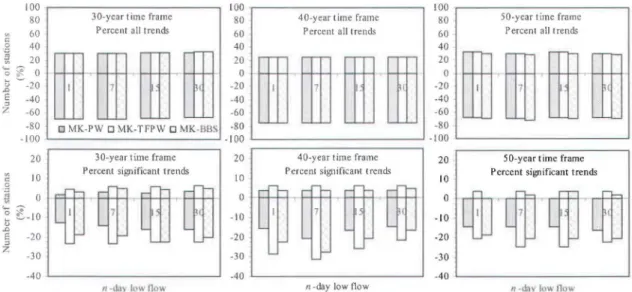
The percent number of stations where positive (increasing) and negative (decreasing) trends in 1-, 7-, 15- and 30-day annuallow flows for the three studied time frames are shown in Figure 3 (top panels). The positive and negative nature of the trend is decided on the basis ofthe sign of the MK test statistic. However, one could also obtain similar results using the SS method, but those results may not always exactly be the same. From zero to a maximum of 4% difference (with a small average difference of 0.4%), between the results of the MK and

SS methods, has been noticed in the present study when deciding the nature of the trend. The results of Figure 3 suggest that for the 40-year time frame, the proportion of positive (negative) trends is slightly smaller (larger) than the corresponding proportions for the 30-year and 50-year time frames. In general, as far as the nature of trend is concerned, the results obtained with the MK-PW, MK-TFPW and MK-BBS approaches are very similar, with about two thirds of the RHBN stations suggesting negative trends and the remaining one third suggesting positive trends.

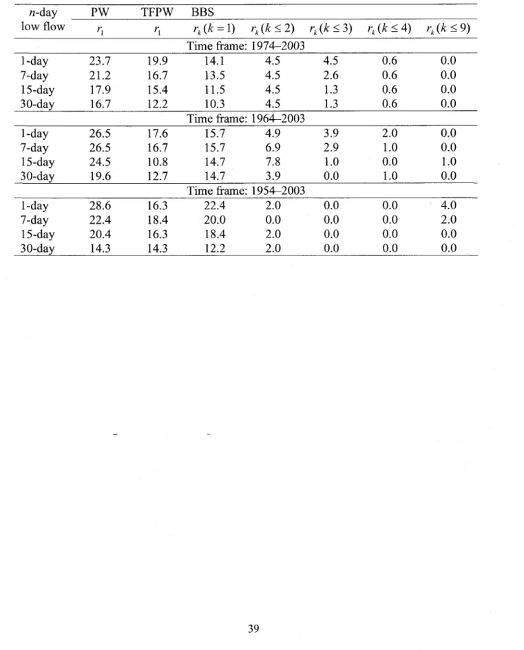
The significance of the observed trends estimated with the MK-PW, MK-TFPW and MK-BBS approaches differs from each other, particularly for the cases of significantly autocorrelated time series. Therefore, it is important to know information about the seriaI structure of time series of various n-day low flows. The percent number of annual n-day low flow time series which exhibit significant auto correlation coefficients of order k (k 21) for three studied time frames are given in Table 1. It should be noted that the auto correlation coefficients for the PW and BBS approaches are obtained from the raw data samples for the autocorrelated time series and not from the transformed data as for the TFPW approach. The percent number of time series which show significant autocorrelation coefficients of order one is higher for the PW and BBS approaches as compared to the TFPW approach for the four annual n-day low flow time series for the three time frames studied. In general, the percent number of time series with significant autocorrelations is highest for 1-day low flows and lowest for 30-day low flows, irrespective of the approach of analysis for incorporating the effect of autocorrelations. It is also interesting to notice from Table 1 that a non-negligible number of low flow time series exhibit significant autocorrelation coefficients of order higher

than one, particularly for the 30- and 40-year time frames. The PW and TFPW approaches assume that these autocorrelation coefficients are negligible.

The percent number of stations which show statistically significant positive and negative trends in the time series of the selected four annual n-day low flows for the three studied time frames obtained with the MK-PW, MK-TFPW and MK-BBS approaches are shown in bottom panels of Figure 3, where differences between the results ofthese approaches are especially evident. The following main conclusions can be drawn from the results presented in this figure:

(1) The MK-PW approach is more conservative in identifying stations with significant trends as compared to the other two. Thus, the stations with weak signaIs would be overlooked by this approach; this observation confirms the previously reported results [Yue et al., 2002b] based on Monte Carlo simulation experiments.

(2) The MK-BBS approach give results that lie in between those obtained with the MK-PW and MK-TFPW. The possible reason behind this could be explained as follows. The MK-TFPW approach neglects the effects ofhigher order significant autocorrelations and that could result in higher number of significant trends. In addition to neglecting the effects of higher order significant autocorrelations, more importantly, the PW approach affects the slope of the original data values and hence the ability of the MK test to identify significant trends [Yue et al., 2002b; Fleming and Clark, 2002]; this could result in lower number of significant trends. The MK-BBS approach does not suffer from these problems and almost exactly takes into account the short-term auto correlation structure of the time series being tested.

(3) Although 1-, 7-, 15- and 30-day low flow time series are derived from the same dataset for every station of the RHBN, the percent number of stations with significant trends

for each n-day low flow time series is not the same. This point can also be verified from Figure 4 where the number oftime series oflow flows (i.e., out of 1-, 7-, 15- and 30-day low flow time series), for each station, with simultaneously significant trends is shown. It is obvious that the trends in 1-, 7-, 15- and 30-day low flow time series are not found simultaneously significant for many stations. These results suggest that by analyzing only one low flow time series (e.g., I-day low flows), one could have inadvertently led to a different set of conclusions. Thus, the advantage of studying more than one low flow time series, derived form the same dataset, is very obvious.

(4) For the RHBN stations analyzed here, an studied methods indicate that the number of stations with significant negative trends in the selected annual n-day low flows is much greater than the number of stations with significant positive trends, irrespective of the period of analysis.

The results of field significance analysis are presented in Table 2(a). It is found that the annuallow flow regimes in the RHBN are dominated by positive cross correlations. For example, for the annual 7-day low flows for the 30-, 40- and 50-year time frames, the proportion of significant positive (negative) cross correlations is 14% (2%), 15% (2%), and 18% (2%), respectively. Therefore, the results of field significance analysis are robust to the presence of positive cross correlations. Because of the problems (discussed above) associated with the MK-PW and MK-TFPW approaches, here the discussion is limited to the MK-BBS approach only. However, the results for the other two approaches are presented for the sake of completeness. The usefulness of studying more than one low flow regime and more than one time frame is obvious from the results of field significance analysis because the strength of the signal (i.e., the number of discoveries) do vary from one low flow regime to the other and

across various time frames. The results of trend analyses for aIl four low flow regimes are field significant for the 40- and 50-year time frames, while for the 30-year time frame, only the 7- and 15-day low flow regimes are field significant. The strength of the signal is relatively stronger for the 40-year time frame as is obvious from the number of discoveries. For example, for this time frame, the 30-day low flow regimes are significantly changing at 22% of stations (see second bottom panel Figure 3) while field significance test however suggests significant changes at 8% of stations; the time trends at the remaining 14% of stations could be false.

Based on the comparative results discussed above for the MK-PW, MK-TFPW and MK-BBS approaches, it is obvious that the MK-BBS approach incorporates the effects of seriaI dependence in an appropriate manner than the other two and therefore the MK-BBS approach is used for the analyses presented in the rest ofthe paper.

4.1.2. Spatial distributions of temporal trends

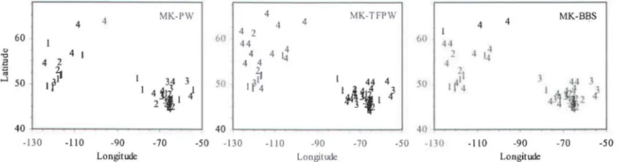
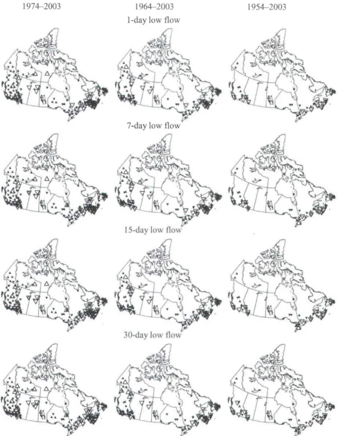
Spatial distributions of time trends in the selected annual n-day low flows for the three time frames obtained with the MK-BBS approach are shown in Figure 5. Collectively over the 1974-2003, 1964-2003 and 1954-2003 time frames, significant negative trends are observed in southem British Columbia, central and southwestem Alberta, central Saskatchewan, southem Ontario and Quebec and Atlantic provinces (New Brunswick, Nova Scotia, Newfoundland and Prince Edward Island). Northem British Columbia, Yukon, Northwest Territories, Nunavut and southem Ontario (Great Lakes region) show significant positive trends. Central British Columbia shows both significant positive and negative trends. It should be noted that these conclusions are drawn from the results for theRHBN and they could vary when such trend analyses are performed on basin-scale using additional stations. As far as the

spatial distributions of non-significant positive and negative trends are concerned, there is no discernable pattern of their occurrence and often both types of trend coexist throughout the RHBN. The spatial distributions of positive and negative trends in 1-day annual low flows, where the MK-PW, MK-TFPW and MK-BBS approaches agree, are broadly in agreement with those previously reported in Zhang et al. [2001] and Yue et al. [2003], who explored annual 1-day low flows for the RHBN but using data till the year 1996 for three different time frames. Analyses of 7-, 15- and 30-day annual low flows were not performed earlier and hence provide additional insights into the temporal evolution of annual low flow regimes in the RHBN. According to the FDR field significance test, discoveries are found in northern and southern British Columbia, central Alberta, southern Ontario and Quebec, New Brunswick and N ewfoundland.

4.2. Win ter season n-day low flows

4.2.1. Temporal trends

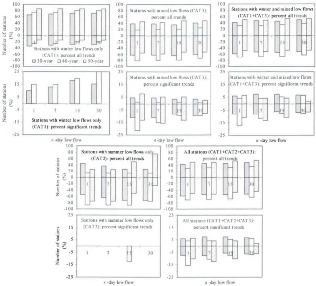
The temporal evolution of winter n-day low flows is studied by partitioning the RHBN stations into three categories namely CATI, CAT2 and CAT3. The numbers of stations, which satisfy the station inclusion criteria presented in the methodology section, for CATI are 39, 20 and 7 for 30-, 40- and 50-year time frames, respectively. In the same order, the number of stations for CAT2 is Il,8 and 4 and that for CAT3 are 106, 74 and 38. The percent number of stations with positive and negative trends in the time series of winter n-day low flows for individual and mixed categories of RHBN stations is shown in Figure 6. The percent number of stations with significant positive and negative trends is also shown in this figure and the following observations can be made from the presented results:

- - -

-(1) Both positive and negative trends (number of positive trends » number of negative trends) are observed in time series of winter n-day low flows for CATI stations but only positive trends are found significant at sorne of the stations for the 30- and 40-year time frames and none for the 50-year time frame. This behavior hints toward a generally increasing pattern ofwinter low flows in the recent past for CATI stations.

(2) Both positive and negative trends (number of negative trends> number of positive trends) are observed in time series ofwinter n-day low flows for CAT3 stations. The percent number of stations with significant negative trends is higher than that with significant positive trends, suggesting that there is no conclusive pattern of trends for CA T3 stations. The same conclusion applies for combined CATI and CAT3 RHBN stations.

(3) Both positive and negative trends, with greater number of negative trends, in winter n-day low flows are observed for CA T2 stations but most of them are not found significant, except few significant negative trends for 15-day low flows only. From these results it can be stated that winter low flows at CA T2 RHBN stations are not experiencing any obvious significant temporal change because of a very weak signal.

(4) The overall results demonstrate that both positive and negative trends, with almost same proportions, exist in the winter n-day low flows for the RHBN.

Based on an analysis of annual or winter n-day low flows for the RHBN stations as one category, i.e. without seasonal classification of stations, it would not have been possible to understand the difference in behavior between CATI and CAT2 stations, with CATI stations experiencing significantly increasing trends and CA T2 stations experiencing generally no trends in winter n-day low flows. The common belief is that winter flows are increasing, which do es not seem to hold everywhere in the RHBN. Therefore, it is important to categorize

catchments in a larger network, such as the RHBN where seasonality of low flow regimes plays an important role, for realistic identification of temporal changes. This is the most important conclusion of this subsection. However, trends in low flow regimes for any of the time frames for both CATI and CAT2 stations are not found field significant. For CAT3 stations, trends in 15-day low flows for the 30-year time frame, 7- and 30-day low flows for the 40-year time frame, and 1- and 7-day low flows for the 50-year time frame are found field significant.

4.2.2. Spatial distributions of temporal trends

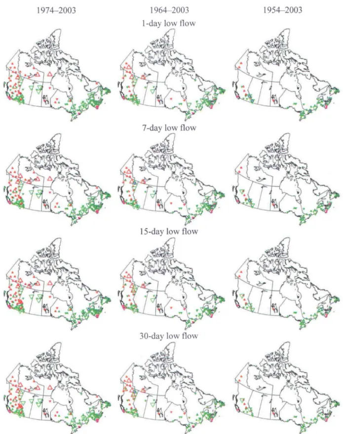
Spatial distributions of positive and negative time trends in winter n-day low flows are shown in Figure 7. It should be noted that observed trends are not simultaneously significant for all n-day low flows for any chosen time frame. Therefore, the spatial interpretation is based on the combined behavior of trends for the winter n-day low flows for the three time frames studied. Significantly increasing short-term trends are found in central and northem British Columbia, southwestem Alberta, Yukon, Northwest Territories and Nunavut for CATI stations. These increasing trends could be attributed, in a qualitative sense as no quantitative analysis has been undertaken, to increasing winter warming trends reported in the work of Bansal et al. [2001], who found increasing trends in the lower and higher percentiles of the daily minimum and maximum temperature distributions for the December to May period in southwestem Canada, west of 85°W. The analyses presented in ACIA [2005] corroborate the winter warming trends.

For CAT3 stations, significantly decreasing trends are found in central and southem British Columbia, central and southwestem Alberta, central Saskatchewan, southem Quebec, Newfoundland, New Brunswick and Nova Scotia, and significantly increasing trends are

found in southem Ontario and northem British Columbia. On the basis of winter warming trends discussed in the above paragraph, increasing trends could be explained but there is no simple explanation for decreasing trends observed in southwestem Canada for CA T3 stations, which require further investigation particularly on regional-scales. Also, dec1ining trends in historie annual streamflows are observed for rivers in the Canadian Rockies [Raad et al., 2005] and the Canadian Prairies [Westmacatt and Burn, 1997; Yulianti and Burn, 1998]. The decreasing trends observed for CA T3 stations located in southeastem Canada could be due to winter cooling trends reported in Zhang et al. [2000] and Bansal et al. [2001] but this attribution should be considered only qualitative as no quantitative analysis has been undertaken. For CAT2 stations, the only significant decreasing trend is in southwestem British Columbia for the 15-day low flows for the 40-year time frame, suggesting a very weak overall signal. Field significance analysis discaveries are found in northem and southem British Columbia, southwestem Alberta, southem Ontario and Quebec, and Nova Scotia.

4.3. Summer season n-day low flows 4.3.1. Temporal trends

The types of RHBN stations used for the analysis presented in this subsection are the same as for the winter season presented in subsection 4.2. It is necessary to point out here that summer n-day low flows generally terminate on November 30th for many of the CATI and CAT3 stations and therefore 30-day low flows would represent November flows. The hydrographs for these stations gradually dec1ine toward winter season low flows and it is not possible to define an exact ending date for summer low flows.

The percent number of stations with positive and negative trends in the time series of summer n-day low flows for individual and mixed categories of the RHBN stations is shown

III Figure 8, and that with significant trends is also shown III this figure. Following

observations can be made from the results presented in this figure:

(1) Generally negative trends in summer n-day low flows are observed for CAT2 stations, with few exceptions for the 40-year time frame. Significant negative trends exist in time series of summer low flows for the 30-, 40- and 50-year time frames with larger proportions for 1-, 7- and 15-day low flows for the 40-year time frame.

(2) Similar to winter low flows, both positive and negative trends are observed in summer n-day low flows for CA T3 stations but with much larger proportion of stations with negative trends. Generally negative trends are found to be significant for aIl three time frames with few exceptions for the 50-year time frame. In contrast with winter low flows, for which the results are inconclusive, it can be stated that summer n-day low flows are decreasing at CA T3 RHBN stations. The same conclusion applies for combined CA T2 and CA T3 RHBN stations.

(3) For CATI RHBN stations, both positive and negative trends are observed in summer n-day low flows. The number of significant positive and negative trends is very small but significant positive trends dominate.

(4) The overall results demonstrate that both positive and negative trends (with positive proportions «negative proportions) exist in summer n-day low flows for the RHBN. The percent number of stations with significant positive trends is much smaller than the percent number of stations with significant negative trends for aIl n-day low flows and time frames. Thus, the RHBN is dominated by negative trends in summer low flows.

Merely based on the analysis of annual n-day low flows, it would not have been possible to identify that summer low flows are significantly decreasing at CAT2 and CAT3

RHBN stations. The trends in summer low flows for the CATI stations are not field significant for any of the time frame. For the CAT2 stations, the trends in sorne of the n-day low flows are field significant but the number of discaveries is very small (at most one). However, the temporal changes are more obvious for the CAT3 stations, i.e. the trends in

n-day low flows are field significant along with many discaveries.

4.3.2. Spatial distributions of temporal trends

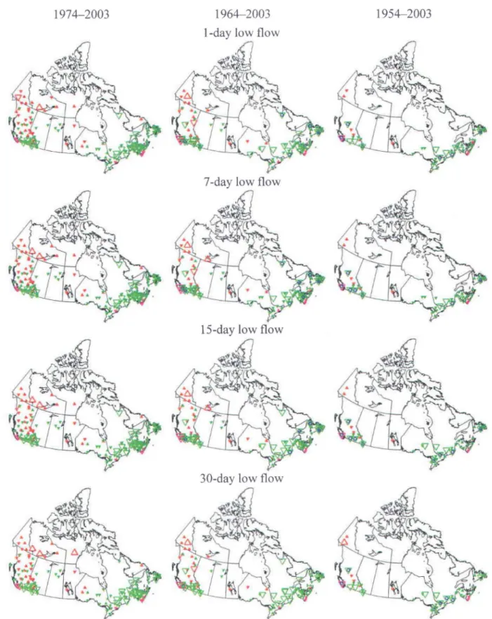
Spatial distributions of positive and negative time trends in summer n-day low flows are shown in Figure 9. Significantly increasing trends are found in Yukon, Northwest Territories, Nunavut and southem British Columbia for CATI stations, but they are not simultaneously significant for the four n-day low flow time series and for the three time frames studied. For the same category of stations, significantly decreasing trends are found in Yukon for the 30-year time frame (l-day low flows) and central British Columbia for the 40-year time frame only.

For CAT3 stations, significantly decreasing trends are found in central and southem British Columbia, southem Alberta and Ontario, northem and southem Quebec, Newfoundland, New Brunswick and Nova Scotia, and significantly increasing trend in southem Ontario for the 50-year time frame only. For CAT2 stations, significantly decreasing trends are found in southwestem British Columbia and Nova Scotia only. According to Bansal et al. [2005], southem Canada, where aIl of the CAT2 and most of the CAT3 stations are located, is associated with significant trends towards fewer days with extreme low temperatures during summer for the 1900-1998 and 1950-1998 periods, compared to daily maximum temperatures, for which consistent changes were not noticed. It is plausible to qualitatively postulate that the above reported warming of the summer low temperature

regime is partially responsible for the decreasing trends in low flow regimes for the CAT2 and CAT3 stations. Field significance analysis discoveries for CAT3 stations are found in central and southem British Columbia, southem Alberta and Ontario, northem and southem Quebec, Newfoundland and New Brunswick. While those for the CAT2 stations are found in Nova Scotia and southwestem British Columbia.

4.4. Choice of time frame and long-term persistence (L TP)

4.4.1. Choice of time frame

The effect of time frame on the estimated trends is analyzed by selecting only 10 RHBN stations with longer records, ranging from 75 to 93 years, and estimating consecutive trends using 30-, 40- and 50-year moving windows. Most of the RHBN stations with record length > 80 years are concentrated in southem Canada, particularly in Ontario (5 stations), New Brunswick (3 stations) and Nova Scotia (6 stations). Two of the selected 10 stations belong to CAT2 and the remaining 8 to CAT3, including one station from Quebec and another from Newfoundland with record length of 75 and 77 years, respectively. No long-term station is available for CATI. Time evolutions of trends in time series of 1-, 7-, 15- and 30-day winter and summer low flows were obtained and those for only winter 7-day low flows are shown in Figure 10 for brevity. Depending on the chosen time frame, both positive and

-

-negative trends exist within the full record of observations for the same time series. Also, it can be seen that trends systematically change from positive to negative and vice versa. This reveals a tendency towards fluctuating behavior, i.e. many drought-rich years follow many drought-poor years (and vice versa) to produce a systematic behavior. It is possible that the systematic fluctuating behavior in low flow regimes may have associations with the large scale atmospheric circulation anomalies, including El Nino--Southem Oscillation, the North

- - -

-Atlantic Oscillation, the Pacific Decadal Oscillation, or the Arctic Oscillation, and it would be interesting to explore such associations in future to better understand the behavior of low flow regimes in Canadian rivers.

The positive trends for the full historical observations for stations 02EC002 and 02KB001 are found to be significant while the trends in observations for the 1974-2003, 1964-2003 and 1954-2003 time frames are not significant. Therefore, the estimated trends in observations of low flows for the past 30-50 years cannot be reliably assumed as representative of long-term trends. These observations suggest that the positive and negative nature of trends and their associated temporal and spatial interpretation appear to be closely tied with the chosen time frames. Given the history of evolution of temporal trends for the long-term stations, it is difficult to be certain if the temporal and spatial patterns of trends observed for the 1974-2003, 1964-2003 and 1954-2003 time frames will continue to persist into the future. Because of the sensitivity of trends to the chosen time frame, care must be exercised in the comparison and interpretation of trends in low flow regimes with corresponding trends in precipitation and temperature.

4.4.2. Long-term persistence (L TP)

In sorne earlier [e.g., Potter, 1976] and recent studies [e.g., Koutsoyiannis, 2003; Cohn and Lins, 2005; Mil/s, 2007] it has been suggested that the above presented fluctuating behavior of trends is a manifestation of L TP. Thus, it becomes important to investigate the presence/absence of LTP in time series of low flow regimes because it has significant impact on the interpretation of trends identified with the assumption of STP. The presence of LTP is usually investigated by estimating the Hurst exponent H; 0.5 < H < 1 range corresponds to a persistent process, 0 < H < 0.5 range corresponds to an antipersistent process and H

=

0.5

corresponds to a purely independent process. Various methods have been developed to estimate the Burst exponent, in addition to the rescaled range statistic (commonly known as RIS) originally proposed by Hurst [1951]. For an overview ofthese methods, see Taqqu et al. [1995]. Most ofthese methods are intuitive and easy to apply. In this study, three commonly used techniques are investigated; Proc1: rescaled adjusted range statistic [Mielniczuk and Wojdyllo, 2007], Proc2: aggregated standard deviation [Koutsoyiannis, 2003, 2006], and Proc3: fractional autoregressive integrated moving average (FARIMA (p,d,q)) modeling approach [Hosking, 1984], where p and q respectively stand for the number of autoregressive and moving average parameters and d

=

H - 0.5 is the fractional differencing parameter. Details of these procedures can be found in the respective references. It is noted that Hosking [1984] has recommended at least 100 years of record to investigate LTP. In hydrology, instrumental river flow records seldom exceed 100 years and therefore records do not satisfy the condition for a long-term data. As a result of this fact, it becomes important to study the sampling distribution of H in order to establish Monte Carlo simulation confidence intervals for diagnostic purposes. To establish whether the value of H estimated with each of the three selected methods for a given sample is significantly different from 0.5, Monte Carlo simulated distribution of His developed by generating a large number of random samples, each of size equal to the observed one, from a white noise process (i.e., normally distributed values with zero mean and unit variance) and estimating H for each of the simulated samples. The results of this analysis are shown in Figure 11. For the FARIMA (p,d,q) model with p

s

q

sI,

FARIMA (O,d,O) mode! is found as the best fitting model for majority of the low flow time series (z 50 years long) on the basis of Bayesian information criterion [Schwarz, 1978] and therefore the corresponding results for the F ARIMA (0, d ,0) are adopted for presentation. For

F ARIMA modeling and simulation, the 'fracdiff' package of the 'R' computing environment is used. On the basis of 95% confidence intervals obtained using Proc1 for estimating H, 7-day winter low flows do not exhibit LTP. When Proc2 and Proc3 are used, the number of stations which possibly exhibit LTP are one (i.e., 05BBOOl) and 3 (i.e., OlAQOOl, 02PJ007 and 05BBOOl) respectively. These results clearly demonstrate that an estimated value of H different from 0.5 (see Figure 11) does not necessarily mean LTP and so care must be exercised in its interpretation, particularly when H is estimated from short sampI es. Sorne other conclusions can also be drawn from Figure Il, e.g. the distribution of H can easily be assumed Normal, the value of H when estimated using Proc1 is biased upward and that when estimated using Proc2 and Proc3 is biased downward. Sorne of these results are consistent with the findings of Couillard and Davison [2005]. It is also worth mentioning here that much narrower confidence intervals for H are noted for large samples indicating that the degree with which one can confidently diagnose LTP increases with the increase in sample size; see Couillard and Davison [2005] for details on diagnosing LTP and for sorne statistical tests and related discussion.

If it is assumed that L TP is present in time series of low flow regimes then it has profound influence on the interpretation of the results presented in earlier sections of the paper under the assumption of STP. For example, for station 02EC002 for which there is insufficient evidence in favor of L TP on the basis of Monte Carlo simulated confidence intervals, the p-value of the trend identification test increased by several orders of magnitude but still remained significant, i.e. from 0.005 (obtained using the MK-BBS approach) to 0.02. Similarly, for station 02PJ007 for which LTP could possibly be assumed, the p-value again increased from 0.22 (obtained using the MK-BBS approach) to 0.40. In general, these results

are consistent with the ones presented in Cohn and Lins [2005] and Koutsoyiannis [2003]. For assessing the significance of the observed MK test statistic under the assumption of L TP, the following simple stochastic simulation procedure is adopted: (1) fit a F ARIMA (0, d ,0) model with 0 < d < 0.5 to observations of low flows, (2) generate a sample from the fitted FARIMA(O,d,O) model of size equal to the observed record and estimate the MK test statistic, (3) repeat step (2) for a large number of times to develop a simulated distribution of the MK test statistic, (4) estimate the significance of the observed MK test statistic from the simulated distribution developed in step (3). This procedure is similar in spirit to the ones presented in Cohn and Lins [2005] and Koutsoyiannis [2003]. Other stochastic modeling and simulation methodologies like the one developed in Langousis and Koutsoyiannis [2006] could also be employed. Following the ab ove described simulation procedure, the estimated trends in annual, winter (for CA T3 stations) and summer (for CA T3 stations) low flow regimes for the 50-year time frame are analyzed and subjected to field significance analysis. Contrary to the results presented in Tables 2(a) to 2(c) for the STP case, none of these low flow regimes is found field significant and the number of stations with significant trends reduced on average by 9.7% for annual, 7.9% for winter and 8.6% for summer low flows.

5. DISCUSSION

The sensitivity of streamflows to changes in climatic inputs is weIl known and it is thus important to look for evidence of temporal changes in various streamflow regimes. A temporal change could be in the form of a monotonic trend or a sudden jump or a combination ofboth ofthem. In this study, the temporal changes in 1-, 7-, 15- and 30-day low flow regimes of the Canadian RHBN is assumed to be in the form of a monotonic trend, which could be

linear, and no attempt has been made to investigate other forms of the temporal change. Low flow regimes corresponding to various durations are considered because the conclusions drawn from the analysis of I-day low flows do not hold true for low flows of 15- and 30-day durations across the whole network.

It is shown in this study that annuallow flows reveal seasonal behavior, i.e. low flows are caused by two distinct physical mechanisms. Thus, to take into account the effect of seasonal behavior of low flows appropriately, the RHBN is divided into three types of stations: (1) stations where annuallow flows were observed during the winter season only (2) stations where annual low flows were observed during the summer season only, and (3) stations where annual low flows were observed both during the winter and summer seasons. This partitioning of the RHBN stations is imperative because results of the study show that conclusions drawn from the analysis of annuallow flows alone, without due consideration to their seasonal behavior, could lead to erroneous conclusions for the whole network. Therefore, the seasonality of the studied low flow regimes should not be ignored when identifying temporal changes.

Numerous studies have investigated patterns of temporal trend in streamflow regimes but there is no general agreement among hydrologists on the best methods to identify trends. The adopted methods included non-parametric, parametric, Bayesian and resampling procedures. This study employed the MK nonparametric test in combination with the PW, TFPW and BBS approaches to incorporate the effect of STP in order to study temporal evolution of low flow regimes in Canadian rivers. The combined MK-BBS approach, while being simple, is based on least number of statistical assumptions and properly takes into account the effect of auto correlation structure of the time series of low flows. The

auto correlation structure of the time series being tested is known to affect the accuracy of the trend identification methods. The issue of selection and use of an appropriate methodology for assessing temporal changes in hydrological time series is an important one and it will continue to attract additional research because the results of estimating trend significance are not only sensitive to the choice of the method but also to the assumptions about the seriaI structure of the time series. It is also instructive to use more than one method for satisfactorily assessing the temporal change signal from limited length hydrological records. At the outset of any trend investigation study for detecting changes in time series of hydrological records, simple approaches involving least number of statistical assumptions, either based on the STP or LTP hypothesis, should be used and then the recourse be made to other sophisticated approaches, such as the ones reviewed in Khaliq et al. [2006], for modeling purposes to develop non-stationary low flow magnitude-frequency relationships.

Under the assumption of STP, both statistically significant increasing and decreasing trends are noticed in low flow regimes in different parts of Canada, but the exact nature of causes of these trends has not been investigated. A detailed analysis ofthe interaction between climatic factors and low flow regimes is beyond the scope of this paper and therefore plausible qualitative explanations based on previously published work on trends in the associated climate fields for increasing and decreasing trends in low flow regimes are provided. Although the RHBN provides an excellent datas et for studying temporal changes, the limited record length and poor spatial coverage, especially in northern Canada, are obvious limitations. The interpretation of trends is strongly tied with the time period analyzed which makes it difficult to generalize the inferences made from 30-50 years datasets as there is potential for errors to be introduced depending on whether the period considered is

drought-rich or drought-poor. Therefore, it is difficult to assume that the observed trends in low flow regimes and their joint spatial patterns for the 30-, 40- and 50-year time frames noted in the study reflect the behavior of longer time frames in all regions of the country.

The assumption of L TP as opposed to STP when identifying hydrological trends is another important issue that needs special attention because not only the at-site but also collective interpretation of identified trends is affected by this assumption. For example, for the 50-year time frame, the trends in 7-day summer low flows for the CAT3 stations are field significant under the assumption of STP but are not field significant under the assumption of LTP. In order to satisfactorily diagnose the presence/absence of LTP, very long observed records are required but hydrological records seldom exceed 100 years and therefore do not satisfy the requirement of very long records. Analysis of 10 relatively long records (which vary between 75 and 93 years) from the RHBN demonstrates that it is not advisable to decide the presence/absence of LTP merely based on the estimated value of the Hurst exponent, particularly when it is estimated from records which do not satisfy the requirement of very long record. Therefore, the Hurst exponent estimated from observed hydrological records should be subjected to statistical testing to identify satisfactorily the presence/absence ofLTP.

Finally, the results ofthis study have enhanced our knowledge concerning evolution of temporal changes in low flow regimes of Canadian rivers, in addition to a better understanding of the methods used for investigating trends under the assumption of STP. The observed trends in low flow regimes, where they are found field significant, could be seen as potential evidence of climate change and its impact on the hydrological cycle, which could eventually lead to shifts in water resources management strategies. Further research into the attribution of the observed trends on basin-scale is needed, because of the regional differences observed in

the evolution of low flowregimes. In particular, the links to local climate and indices of large scale atmospheric circulations would be useful to better understand the past changes and variability in the low flow regimes of Canadian rivers. Furthermore, the effect of cross correlation, if it is responsible for generating false discoveries, can best be studied by defining small hydrological homogeneous regions or climatic zones. Lastly, it should not be forgotten that the interpretation of identified trends, whether at local or regional scales, is strongly dependent on the assumption of STP/LTP and more importantly on how well the assumption of LTP can be verified from limited length hydrological records.

ACKNOWLEDGEMENTS

The financial support provided by the Ouranos Consortium on Regional Climatology and Adaptation to Climate Change, National Science and Engineering Research Council (NSERC) of Canada and Environment Canada (Adaptation and Impacts Research Division) is gratefully acknowledged. The authors would like to thank Andreas Langousis, Francesco Laio and Harry Lins, and the Associate Editor, Demetris Koutsoyiannis, for helpful comments.

REFERENCES

ACIA (Arctic Climate Impact Assessment) (2005), Impacts of a warming Arctic: Arctic Climate Impact Assessment, Scientific Report, 1042 pp., Cambridge University Press, Cambridge, available on: http://www.acia.uaf.edu. date visited: March 10,2007.

Benjamini, Y., and Y. Hochberg (1995), Controlling the false discovery rate: A practical and powerful approach to multiple testing. J. R. Statist. Soc., Ser. B, 57,289-300.

Bonsal, B.R., X. Zhang, L.A. Vincent, and W.D. Hogg (2001), Characteristics of daily and extreme temperatures over Canada, J. Clim., 14, 1959-1976.

Brimley, B., J.F. Cantin, D. Harvey, M. Kowalchuk, P. Marsh, T.B.M.J. Ouarda, B. Phinney, P. Pilon, M. Renouf, B. Tassone, R. Wedel, and T. Yuzyk (1999), Establishment of the referenee hydrometrie basin network (RHBN) , Environment Canada Researeh Report, 41 pp., Ontario, Canada.

Bum, D.H., and M.A. Hag Elnur (2002), Detection of hydrologie trends and variability, J Hydra/., 255, 107-122.

Chiew, F.H., and T.A. McMahon (1993), Detection of trend in or change in annual flow of Australian rivers, Int. J. Climatal., 13,643-653.

Cohn, T.A., and H.F. Lins (2005), Nature's style: Naturally trendy, Geoph. Res. Let, 32, doi: 10.1029/2005GL024476.

Couillard, M., and M. Davison (2005), A comment on measuring the Hurst exponent of financial time series, Pysica A, 384, 404-418.

Dahmen, E.R., and M.J. Hall (1990), Screening of Hydrological Data, Publication No. 49, 58 pp., International Institute for Land Reclamation and Improvement (ILRI), Netherlands. Davison, A.C., and D.V. Hinkley (1997), Bootstrap Methods and their Application,

Cambridge University Press, Cambridge.

- Déry, S.J., and E.F. Wood (2005), Decreasing river discharge in northem Canada, Geophys. Res. Lett. 32, LI0401, doi: 10.l029/2005GL022845.

Douglas, E.M., R.M. Vogel, and C.N. Knoll (2000), Trends in flood and low flows in the United States: impact of spatial correlation, J Hydral., 240, 90-105.

Elmore, K.L., M.E. Baldwin, and D.M. Schultz (2006), Field significance revisited: Spatial bias errors in forecasts as applied to the Eta model. Mon. Weath. Rev., 134,519-531.

Fleming, S.W., and G.K.C. Clark (2002), Autoregressive noise, deserialization, and trend detection and quantification in annual river discharge time series, Cano Water Resour. J., 27(3), 335-354.

Gan, T.Y. (1998), Hydroc1imatic trends and possible c1imatic warming in the Canadian Prairies, Water Resour. Res., 34(11), 3009-3015.

Gustard, A., A. Bullock, and J.M. Dixon (1992), Low flow estimation in the United Kingdom, IH Report No. 108,88 pp., Institute of Hydrology, Wallingford, Oxon.

Hannaford, J., and T. Marsh (2006), An assessment of trends in UK runoff and low flows using a network of undisturbed catchments, Int. J. Climatol., 26, 1237-1253.

Harvey, K.D., P.J. Pilon, and T.R. Yuzyk (1999), Canada's reference hydrometric basin network (RHBN): In partnerships in water resources management, paper presented at Canadian Water Resources Association (CWRA)'s 51 st annual conference, Halifax, Nova Scotia, June 1999.

Hisdal, H., K. Stahl, L.M. Tallaksen, and S. Demuth (2001), Have streamflow droughts in Europe become more severe or frequent? Int. J. Climatol., 21,317-333.

Hosking, J.R.M. (1984), Modeling persistence in hydrological time series usmg usmg fractional differencing, Water Resour. Res., 20(12), 1898-1908.

Hurst, H.E. (1951), Long term storage capacity of reservoirs. Trans. ASCE, 116, 776-808. IPCC (2001), Climate Change 2001, Synthesis Report, edited by RT Watson and the Core

Writing Team, Contribution of Working Groups l, II and III to the Third Assessment Report of the Intergovernmental Panel on Climate Change (IPCC), Cambridge University Press, Cambridge.