Analytic Solution to Optimal Reconfigurations of Satellite Formation Flying in Circular Orbit under J2 Perturbation

(1)

Analytic Solution to Optimal

Reconfigurations of Satellite

Formation Flying in Circular

Orbit under J

2 Perturbation

HANCHEOL CHO SANG-YOUNG PARK HAN-EARL PARK KYU-HONG CHOI Yonsei University Republic of Korea

This paper presents an analytic solution to the optimal reconfiguration problem of satellite formation flying in J₂orbital perturbation. Continuous and variable low-thrust accelerations are represented by the Fourier series, and initial and final boundary conditions are used to establish the constraints on the thrust functions. The thrust functions are implemented by optimal Fourier coefficients that minimize the cost during the maneuver. The analytic solution composed of these Fourier coefficients are simply represented in a closed form, and no approximation is needed. Numerical simulations are conducted to visualize and compare the results obtained in this paper with those of previous papers with no perturbations. The analytic solution developed in this paper is more accurate in that the general behavior of the optimal control history and reconfiguration trajectories are easily calculated even in the presence of the J₂potential disturbance. The analytic solution is useful for designing a reconfiguration controller for satellite formation flying under J₂orbital perturbation.

Manuscript received May 8, 2008; revised December 24, 2008, July 3, 2009, and November 4, 2009; released for publication July 21, 2011.

IEEE Log No. T-AES/48/3/944010.

Refereeing of this contribution was handled by M. Campbell. This work is supported by the Korean Science and Engineering Foundation through the National Research Laboratory Program funded by the Ministry of Science and Technology (No. M10600000282-06J0000-28210).

Authors’ address: Astrodynamics and Control Laboratory, Department of Astronomy, Yonsei University, Seoul 120-749, Republic of Korea, E-mail: (spark624@yonsei.ac.kr).

0018-9251/12/$26.00 c° 2012 IEEE

I. INTRODUCTION

Satellite formation flying is used when a group of satellites needs to perform a unified space mission. Satellite formation flying has been extensively studied to enable space missions to obtain higher-resolution imagery and interferometry, robust and redundant fault-tolerant space systems, and more complex networks of satellites [1]. Among the technologies associated with satellites in a formation, the optimal reconfiguration problem is of great concern. This is because small satellites consisting of a formation generally have a limited fuel budget. Originally, the Hill-Clohessy-Wiltshire (HCW) equations [2, 3] of relative motion were used to analyze relative motion among satellites because they are the simplest models governing the dynamics of relative motion; these equations model relative motion in a local vertical, local horizontal (LVLH) frame. The HCW equations assume that 1) the reference orbit is circular, 2) the satellites (the chief and the deputy) orbit in the absence of perturbations, and 3) the differential gravity field is linear. If the chief’s orbit is eccentric, if the gravitational field is perturbed, or if the relative distance is not small, then the HCW equations are no longer valid.

The problems associated with relative motion under perturbations have attracted a lot of researchers. Among the various perturbations, the dominant one is Earth’s oblateness, especially the second spherical harmonic of Earth’s geopotential, called J₂[4]. Kechichian [5] derives an exact formulation of the relative motion of satellites under the J₂disturbance, which requires numerical integration to predict the motion of the satellites over time. Sedwick, et al. [6] includes the effects of the J₂ disturbance as a forcing function that they apply to the right side of the HCW equations. This causes the secular drift, and they present the amount of changes in velocity needed to counteract this secular term. Recently, Hamel and de Lafontaine [7] propose a linearized set of equations of relative motion concerning the J₂-perturbed elliptic reference orbit. The model uses the linearized differential drift rate of mean orbit elements to predict the impact of the J₂perturbation on relative osculating satellite motion. However, the most frequently used models that describe relative motion under the J₂ perturbation are those presented by Schweighart and Sedwick [8] and Ross [9]; both of which use the circular reference orbit. The equations proposed by Schweighart and Sedwick were chosen for this paper because they are easily solved and they pick up where Ross leaves off; that is, they account for the shift in orbital period and ascending node associated with the J₂ effect.

(2)

Let us turn to the optimal reconfiguration problem. This problem, which is directly related to the traditional optimal rendezvous problem, is also of great interest, especially because of Lawden’s primer vector theory [10]. Most solutions have been numerically obtained because this problem is highly nonlinear. Zanon and Campbell [11] describe a numerical method for constructing formation optimal maneuvers using the Hamilton-Jacobi-Bellman formulation. Tillerson, et al. [12] present optimal control algorithms for formation keeping and reconfiguration, which are based on the solutions of linear and integer programming. Finding the numerical solutions is somewhat difficult because the necessary and optimality conditions must be numerically satisfied. However, analytic solutions would give insight into the feedback controller, and therefore would be easily exploited for formation flying, if they could be uncovered. Also, for the actual on-board control system, it is preferable to have analytic solutions because this makes the computational load smaller. Vaddi, et al. [13] propose an analytic two-impulse solution using Gauss’s variational equations. This algorithm is based on the circular reference orbit given by the HCW equations. Palmer [14] presents an elegant analytic solution for the problem by representing the continuous and variable thrust acceleration in a Fourier series with a period equal to the maneuver time. He uses Parseval’s theorem [15] to make the infinite sum into a closed form. However, this analytic solution is limited to formation flying in an unperturbed circular orbit because the HCW equations are used. Using a similar approach, Cho, et al. [16] extend the previous result and obtain a solution to general-elliptic-orbit cases. In [16], the Tschauner-Hempel equations [17] are used to describe relative motion in an eccentric orbit, and its fundamental matrix, given by Yamanaka and Ankersen [18], is used. Scott and Spencer [19] choose the calculus of variations to obtain an analytic solution; they bring in the adjoint system to find an optimal thrust vector. This solution applies only to unperturbed circular-reference-orbit cases. Sharma, et al. [20] solve the problem of frequently used eccentricity and include the effects of nonlinear differential gravity.

The control strategy for reconfiguration in the presence of the J₂ disturbance has also been conducted by various researchers. Schaub and Alfriend [21] discuss the effect of applying impulsive control on the orbital elements, perturbed by the J₂ effect. In [22], two approaches–impulsive control and continuous control–are developed and compared. The optimal impulsive controls are obtained from a numerical method, and the continuous controls law is derived from a candidate Lyapunov function. Horneman [23] develops a multi-impulse guidance

scheme in the HCW frame for satellites flying in formation based on a set of relative orbital elements, including first-order effects of the J₂perturbations. However, an analytic solution for fuel-optimal reconfiguration is rarely presented. Yan and Alfriend [24] show an approximate, analytic, low-thrust control law using a pseudospectral method. The control law is based on a state transition matrix, including the J₂ perturbations for linearized equations of relative motion. The control law requires state values to evaluate the control value at the current time, and the values of the control between parameterized points should be obtained by interpolation. However, as evident in [24], this study shows only an approximate control law for formation reconfigurations. Thus, it is challenging to find a method that can be used to obtain analytic solutions of state histories and cost function, as well as control histories for formation reconfigurations under the J₂ perturbations.

We present an analytic solution to the satellite formation reconfiguration (relocation) problem in a J₂-perturbed circular orbit using the Fourier series. The procedure used in this paper to obtain the analytic solution depends on that found in [14]. However, we use a different dynamic model to include the J₂ orbital perturbations, and it obtains an analytic solution that has been modified appropriately. The J₂ perturbations yield stronger effects near the bulge of Earth, which means small orbital inclinations. Hence, when the orbital inclination of the satellite is small, our dynamic model used would be more accurate than the HCW dynamic model in [14]. Consequently, our dynamic model gives more accurate results in control simulation at small inclinations. The analytic method developed in this paper yields closed forms of accelerations, closed forms of position and velocity vectors, and a closed form of cost

function. Initial and final positions and velocities of the deputy satellites are calculated to establish the constraints on the thrust functions. These constraints are incorporated into the cost function by introducing Lagrange multipliers. The analytic solutions are formed by the magnitude and direction of continuous thrust accelerations as a function of time. Presumably, there are no restrictions on the thrust vector, and a transfer time is chosen as a specific value. The satellites are assumed to have low-level thrusters in three orthogonal directions that correspond to the radial, along-track, and cross-track directions. Thrusters are fired during a significant fraction of an orbital period throughout the maneuver. Any thruster acceleration can be represented by the infinite Fourier series. With Parseval’s theorem, the Fourier series is summed up in a closed-form solution. Analytic optimal solutions are derived by using an extreme cost function with respect to all Fourier coefficients. Then, the solution minimizes propellant

(3)

usage for the reconfiguration of satellite formation. The present paper describes thrust accelerations in closed form for the optimal satellite relocation problem. The solution is useful for designing a feedback controller for satellite formation flying in a J₂-perturbed circular orbit. This study has addressed multiple challenges, which are described here. First, for formation reconfigurations, closed form solutions to the circular orbits with J₂ perturbations are found. The analytic solutions include state histories and cost function, as well as control histories. Second, to provide the range of when our solutions play an important role, the dynamic model used is compared to a true nonlinear dynamic model including J₂ perturbations. The underestimated drifts in both the dynamic model used in this study and the dynamic model used in [14] are calculated. Third, we evaluate the accuracy of the solutions both in this paper and in [14] for various orbits. For an inclination of less than i_ref_{¼ 54:735 deg, the solutions calculated here yield} smaller errors of final position than those found in [14]. The new solutions can be used as a baseline in the design of formation flying with an inclination of less than i_ref_{¼ 54:735 deg.}

II. RELATIVE ORBITAL DYNAMICS UNDER J₂ DISTURBANCE

In this section, relative dynamics in the presence of J₂ disturbance is briefly described. Schweighart and Sedwick [8] modify the HCW equations to catch the effect of the J₂disturbance as follows:

¨x ¡ 2np1 + s _y_{¡ (3 + 5s)n}2x = T_x (1a)

¨y + 2np1 + s _x = T_y (1b)

¨z + q2_{z = 2lq cos(qt + Á) + T} z (1c) where the x(t)-axis lies in the radial direction, the y(t)-axis is in the in-track direction, and the z(t)-axis along the orbital angular momentum vector completes a right-handed system, while the dot² above a variable represents the differentiation with respect to time t. In (1), n is the mean motion of the chief satellite, Á is the phase difference between the chief and the deputy satellite at the initial location, the constant s emerges because of the shift of period of a reference orbit, and q, which is also a constant, is responsible for the change of the ascending node in the presence of the J₂ disturbance. Presumably, the thrust functions T_x(t), T_y(t), and T_z(t) can be applied at the desired directions during the maneuver. The equations in (1) are initialized; that is, the cluster of satellites passes the ascending node at t = 0. Let us define t_i and t_f as the turn-on and turn-off points of the thrusters, respectively. Furthermore, the following

are defined [8]: s =3J2R2e 8r2 ref (1 + 3 cos 2i_ref) c =p1 + s, n = r_¹ r3 ref k = nc +3nJ2R 2 e 2r2 ref cos2i_ref i_D= _z0 kr_ref+ iC, ¢−0= z₀ r_refsin i_ref °₀= cot¡1

·

cot iCsin iD¡ cosiDcos ¢−0

sin ¢−₀

¸

©₀= cos¡1[cos iDcos iC+ sin iDsin iCcos ¢−0]

_ −D=¡ 3nJ₂R2 e 2r2 ref cos iD _ −C=¡ 3nJ₂R2 e 2r2 ref cos iC

q = nc¡ (cos°0sin °0cot ¢−0¡ sin 2_°

0cos iD)

£ ( _−D¡ _−C)¡ _−Dcos iD

l =¡rref

sin iDsin iCsin ¢−0

sin ©₀ ( _−D¡ _−C)

m sin Á = z₀, l sin Á + qm cos Á = _z₀

(2)

where the subscripts C and D mean the chief and deputy satellites, respectively, J₂is the second spherical harmonic of Earth’s geopotential, and R_e is the radius of Earth. In addition, r_ref is the radius of the reference orbit, i is the inclination, and ¹_{´ GM}_e, where G is the gravitational constant and M_e is the mass of Earth. s emerges in the process of adjusting the period of the reference orbit to that of the deputy satellite’s orbit, resulting in a new angular velocity of the reference orbit, which is responsible for c. k is employed to force the ascending node of the reference orbit to move at the same speed as the deputy satellite’s orbit. The other quantities are necessary for correcting the cross-track z motion. When c = 1, q = n, and l = 0, the equations in (1) are the same as the familiar HCW equations. Here, we assume that the chief satellite’s orbit coincides with the reference orbit.

III. SOLUTION TO THE MODIFIED HCW EQUATIONS WITH J₂DISTURBANCE

In this section, the solutions to the modified HCW equations in (1) are derived. Because the z motion is decoupled from x and y, the out-of-plane maneuvers are first considered.

A. Solution to Out-of-Plane Maneuvers

First, we solve the homogeneous form of (1c):

(4)

The solution is ·_z h(t) _z_h(t) ¸ = 2 4 cos qt 1 qsin qt ¡q sin qt cos qt 3 5·z0 _z₀ ¸ (4)

where z₀_{´ z(0), _z}₀_{´ _z(0), and the subscript h means} the homogeneous solution. If we want to use the values at the turn-on time t = t_i, we perform the following transformation: ·_z 0 _z₀ ¸ = 2 4 cos qti 1 qsin qti ¡qsin qti cos qti 3 5 ¡1_· z_i _z_i ¸ = 2 4 cos qti ¡ 1 qsin qti q sin qt_i cos qt_i 3 5·zi _z_i ¸ (5)

where z_i_{´ z(t}_i) and _z_i_{´ _z(t}_i). Inserting the J₂ disturbance term 2lq cos(qt + Á) into the right-hand side of (3), the solution is

z_J2(t) = lt sin(qt + Á)

_z_J2(t) = l sin(qt + Á) + qlt cos(qt + Á) (6) where the subscript J2 refers to the particular solution because of the J₂ disturbance term and tan Á = qz₀=_z₀. Next, let us consider another disturbance term: T_z(t). Ignoring the J₂disturbance term, (3) is

¨z + q2_{z = T}

z: (7)

Utilizing the variation of parameters [25], we get z_p(t) =1 q Z t ti sin q(t_{¡ ¿)T}_z(¿ )d¿ and _z_p(t) = Z t ti cos q(t_{¡ ¿)T}_z(¿ )d¿ (8)

where the subscript p means the particular solution because of the thrust term. When t = t_f, the thruster is turned off and the deputy satellite is in the desired relative position; that is, z(t_f) and _z(t_f) are our predefined values, which give the constraints on the thrust function. Therefore, the following constraints must exist at t = t_f: " ˜_I 0 ˜I₁ # ´ ·_z p(tf) _z_p(t_f) ¸ = ·_z(t f) _z(t_f) ¸ ¡ ·_z h(tf) _z_h(t_f) ¸ ¡ ·_z J2(tf) _z_J2(t_f) ¸ : (9)

We then find a thrust function T_z(t) that satisfies (9). B. Solution to In-Plane Maneuvers

We solve the homogeneous form of (1a) and (1b): ¨x ¡ 2np1 + s _y_{¡ (3 + 5s)n}2x = 0

¨y + 2np1 + s _x = 0:

(10) It is straightforward to show that

2 6 6 6 4 x_h(t) _x_h(t) yh(t) _yh(t) 3 7 7 7 5= ©(t, 0) 2 6 6 6 4 x₀ _x₀ y₀ _y₀ 3 7 7 7 5= 2 6 6 6 6 6 6 6 6 6 6 6 6 6 4 1 1¡ s · _{4(1 + s)} ¡(3 + 5s)cos¯t ¸ 1 np1_{¡ s}sin ¯t 0 2p1 + s n(1¡ s)[1¡ cos¯t] n(3 + 5s) p 1_{¡ s} sin ¯t cos ¯t 0 2p1 + s p 1_{¡ s} sin ¯t 2p1 + s(3 + 5s) (1¡ s)p1¡ s [sin ¯t¡ ¯t] 2p1 + s n(1¡ s)[cos ¯t¡ 1] 1 1 1¡ s "4(1 + s) np1¡ ssin ¯t ¡(3 + 5s)t # 2np1 + s(3 + 5s) 1¡ s [cos ¯t¡ 1] ¡ 2p1 + s p 1¡ s sin ¯t 0 1 1¡ s ·_{4(1 + s) cos ¯t} ¡(3 + 5s) ¸ 3 7 7 7 7 7 7 7 7 7 7 7 7 7 5 2 6 6 6 4 x₀ _x₀ y₀ _y₀ 3 7 7 7 5 (11a) where © is the state transition matrix and ¯_{´ n}p1_{¡ s.}

If we use the values at t = t_irather than t = 0, then the following transformation is performed in advance:

2 6 6 6 4 x₀ _x₀ y₀ _y₀ 3 7 7 7 5= © ¡1_(t i, 0) 2 6 6 6 4 x_i _x_i yi _yi 3 7 7 7 5= 2 6 6 6 6 6 6 6 6 6 6 6 6 6 4 1 1¡ s · _{4(1 + s)} ¡(3 + 5s)cos¯ti ¸ ¡ 1 np1¡ ssin ¯ti 0 2p1 + s n(1¡ s)[1¡ cos¯ti] ¡n(3 + 5s)p 1_{¡ s} sin ¯ti cos ¯ti 0 ¡ 2p1 + s p 1_{¡ s} sin ¯ti ¡2 p 1 + s(3 + 5s) (1_{¡ s)}p1_{¡ s} [sin ¯ti¡ ¯ti] 2p1 + s n(1¡ s)[cos ¯ti¡ 1] 1 ¡ 1 1¡ s "4(1 + s) np1¡ ssin ¯ti ¡(3 + 5s)ti # 2np1 + s(3 + 5s) 1¡ s [cos ¯ti¡ 1] 2p1 + s p 1¡ s sin ¯ti 0 1 1¡ s ·_{4(1 + s) cos ¯t} i ¡(3 + 5s) ¸ 3 7 7 7 7 7 7 7 7 7 7 7 7 7 5 2 6 6 6 4 x_i _x_i yi _yi 3 7 7 7 5: (11b)

(5)

Next, the particular solution to (1a) and (1b) must be found. We again use the variation of parameters [25] to get 2 6 6 6 6 4 x_p(t) _x_p(t) y_p(t) _y_p(t) 3 7 7 7 7 5= 2 6 6 6 6 6 6 6 6 6 4 2p1 + s n(1_{¡ s)} ¡ 2p1 + s n(1_{¡ s)} 0 0 0 0 2p1_{¡ s} 0 ¡3 + 5s₁ ¡ s t 0 4p1 + s np1_{¡ s} 1 n(1_{¡ s)} ¡3 + 5s₁ ¡ s 4(1 + s) 1_{¡ s} 0 0 3 7 7 7 7 7 7 7 7 7 5 2 6 6 6 4 I₂(t) I₃(t) I₄(t) I₅(t) 3 7 7 7 5 (12) where I₂(t)_´ Z t ti T_y(¿ )d¿ I₃(t)_´ Z t ti T_y(¿ ) cos ¯(t_{¡ ¿)d¿} ¡ p 1_{¡ s} 2p1 + s Z t ti T_x(¿ ) sin ¯(t_{¡ ¿)d¿} (13) I₄(t)_´ p 1 + s 1_{¡ s} Z t ti T_y(¿ ) sin ¯(t_{¡ ¿)d¿} + 1 2p1_{¡ s} Z t ti T_x(¿ ) cos ¯(t_{¡ ¿)d¿} I₅(t)_{´ n(3 + 5s)} Z t ti T_y(¿ )¿ d¿_{¡ 2}p1 + s Z t ti T_x(¿ )d¿: In (13), ¯_{´ n}p1_{¡ s. The singularity condition of (12)} occurs if 1_{¡ s = 0. However, this singularity rarely} occurs because s = (3J₂R_e2=8r_ref2 )(1 + 3 cos 2i_ref) is rarely 1. As before, constraints must exist at t = t_f:

2 6 6 6 6 4 ˜I₂ ˜I₃ ˜I₄ ˜I₅ 3 7 7 7 7 5´ 2 6 6 6 4 I₂(t_f) I₃(t_f) I₄(t_f) I₅(t_f) 3 7 7 7 5= 2 6 6 6 6 6 6 6 6 6 4 2p1 + s n(1_{¡ s)} ¡ 2p1 + s n(1_{¡ s)} 0 0 0 0 2p1_{¡ s} 0 ¡3 + 5s₁ ¡ s tf 0 4p1 + s np1_{¡ s} 1 np1_{¡ s} ¡3 + 5s₁ ¡ s 4(1 + s) 1_{¡ s} 0 0 3 7 7 7 7 7 7 7 7 7 5 ¡1 2 6 6 6 6 4 x(t_f)_{¡ x}_h(t_f) _x(t_f)_{¡ _x}_h(t_f) y(t_f)_{¡ y}_h(t_f) _y(tf)¡ _yh(tf) 3 7 7 7 7 5 = 2 6 6 6 6 6 6 6 4 2np1 + s 0 0 1 n(3 + 5s) 2p1 + s 0 0 1 0 1 2p1_{¡ s} 0 0 2n2p_{1 + s(3 + 5s)t} f ¡2 p 1 + s n(1_{¡ s) n(3 + 5s)t}_f 3 7 7 7 7 7 7 7 5 2 6 6 6 6 4 x(t_f)_{¡ x}_h(t_f) _x(t_f)_{¡ _x}_h(t_f) y(t_f)_{¡ y}_h(t_f) _y(t_f)_{¡ _y}_h(t_f) 3 7 7 7 7 5 (14)

We then find the thrust functions T_x(t) and T_y(t) that satisfy (14) at t = t_f.

IV. THRUST FUNCTIONS IN A FOURIER SERIES Our objective is to relocate the deputy to the desired position and velocity relative to the chief at t = t_f while minimizing control energy. Therefore, the cost function is J = Z tf ti T2(¿ )d¿ (15) where T2_{(t) = T}2

x(t) + Ty2(t) + Tz2(t) and the low levels of thrusters are operated for the chief satellite’s t_i_· t_{· t}_f. Because the out-of-plane motion is decoupled from the in-plane motion, we divide them into the following two cost functions:

J_z= Z tf ti T_z2(¿ )d¿ (16a) J_xy= Z tf ti [T_x2(¿ ) + T_y2(¿ )]d¿: (16b) Defining ¢t_{´ t}_f_{¡ t}_i, we represent each thrust function as a Fourier series with the period

(6)

of ¢t: T_x(t) =ax0 2 + 1 X n=1 · a_xncos μ_2n¼ ¢t t ¶ + b_xnsin μ_2n¼ ¢t t ¶¸ (17a) T_y(t) =ay0 2 + 1 X n=1 · a_yncos μ 2n¼ ¢t t ¶ + b_ynsin μ 2n¼ ¢t t ¶¸ (17b) T_z(t) =az0 2 + 1 X n=1 · a_zncos μ 2n¼ ¢t t ¶ + b_znsin μ 2n¼ ¢t t ¶¸ (17c) where a_x0= 2 ¢t Z tf ti T_x(¿ )d¿ a_xn= 2 ¢t Z tf ti T_x(¿ ) cos2n¼ ¢t ¿ d¿ b_xn= 2 ¢t Z tf ti T_x(¿ ) sin2n¼ ¢t ¿ d¿ a_y0= 2 ¢t Z tf ti T_y(¿ )d¿ a_yn= 2 ¢t Z tf ti T_y(¿ ) cos2n¼ ¢t ¿ d¿ b_yn= 2 ¢t Z tf ti T_y(¿ ) sin2n¼ ¢t ¿ d¿ a_z0= 2 ¢t Z tf ti T_z(¿ )d¿ a_zn= 2 ¢t Z tf ti T_z(¿ ) cos2n¼ ¢t¿ d¿ b_zn= 2 ¢t Z tf ti T_x(¿ ) sin2n¼ ¢t ¿ d¿:

If Parseval’s theorem [15], which represents the relationship between the average of the square of T(t) and the Fourier coefficients, is used, the cost functions are expressed in terms of the Fourier coefficients:

J_z=¢t 2 " a2_z0 2 + 1 X n=1 (a2_zn+ b2_zn) # (18a) J_xy=¢t 2 " a2_x0 2 + 1 X n=1 (a2_xn+ b2_xn) # +¢t 2 " a2 y0 2 + 1 X n=1 (a2_yn+ b2_yn) # : (18b)

Now, we must find those Fourier coefficients that minimize the cost functions J_z and J_xy. As mentioned earlier, in doing so we must not forget to incorporate boundary constraints. Let us consider the out-of-plane case first and then the in-plane case.

A. Out-of-Plane Optimal Thrust Function

For brevity, we introduce new constraints K₀and K₁ rather than the original constraints of ˜I₀and ˜I₁, respectively: ·_K 0 K₁ ¸ ´ · _{q sin qt} f cos qtf ¡qcosqtf sin qtf ¸" ˜I₀ ˜I₁ # = "Rtf ti Tz(¿ ) cos q¿ d¿ Rtf ti Tz(¿ ) sin q¿ d¿ # : (19)

Substituting (17c) into (19) yields K₀=fz0az0 2 + 1 X n=1 f_za(n)a_zn+ 1 X n=1 f_zb(n)b_zn (20a) K₁=gz0az0 2 + 1 X n=1 g_za(n)a_zn+ 1 X n=1 g_zb(n)b_zn (20b) where f_z0= Z tf ti cos q¿ d¿ f_za(n) = Z tf ti cos q¿ cos2n¼ ¢t ¿ d¿ (21a) f_zb(n) = Z tf ti cos q¿ sin2n¼ ¢t ¿ d¿ g_z0= Z tf ti sin q¿ d¿ g_za(n) = Z tf ti sin q¿ cos2n¼ ¢t ¿ d¿ (21b) g_zb(n) = Z tf ti sin q¿ sin2n¼ ¢t ¿ d¿:

Incorporating the constraints (20) using Lagrange multipliers ¸₀and ¸₁, the augmented cost function J_z,aug obtains the following:

J_z,aug=¢t 2 " a2 z0 2 + 1 X n=1 a2zn+ 1 X n=1 bzn2 # + ¸₀ " K₀¡fz0az0 2 ¡ 1 X n=1 fza(n)azn¡ 1 X n=1 fzb(n)bzn # + ¸₁ " K₁¡gz0az0 2 ¡ 1 X n=1 g_za(n)a_zn¡ 1 X n=1 g_zb(n)b_zn # : (22)

(7)

Then, partially differentiating (22) with respect to each Fourier coefficient a_z0, a_zn, and b_zn, and setting the results equal to zero, the coefficients for the optimal maneuver are obtained as follows to minimize the cost function: a_z0= 1 ¢t[¸0fz0+ ¸1gz0] a_zn= 1 ¢t[¸0fza(n) + ¸1gza(n)] b_zn= 1 ¢t[¸0fzb(n) + ¸1gzb(n)]: (23)

Substituting (23) into (20), K₀ and K₁ are rewritten in terms of ¸₀and ¸₁: " K₀ K₁ # = " p₀ p₁ p₁ q₁ #" ¸₀ ¸₁ # (24) where p₀= f 2 z0 2¢t+ 1 ¢t 1 X n=1 [f_za2(n) + f_zb2(n)] p₁=fz0gz0 2¢t + 1 ¢t 1 X n=1 [f_za(n)g_za(n) + f_zb(n)g_zb(n)] q₁= g 2 z0 2¢t+ 1 ¢t 1 X n=1 [g2_za(n) + g_zb2(n)]:

By Parseval’s theorem, p₀, p₁, and q₁converge at constant values: p₀=1 2 Z tf ti cos2q¿ d¿ =1 2 · ¿ 2+ sin 2q¿ 4q ¸tf ti p₁=1 2 Z tf ti sin q¿ cos q¿ d¿ =1 2 " sin2q¿ 2q #tf ti q₁=1 2 Z tf ti sin2q¿ d¿ =1 2 · ¿ 2¡ sin 2q¿ 4q ¸tf ti where [f(¿ )]tf ti ´ f(tf)¡ f(ti). From (24), we have

convenient closed-form parameters to represent the Lagrange multipliers: ·_¸ 0 ¸₁ ¸ = 1 p₀q₁_{¡ p}2 1 · _q 1 ¡p1 ¡p1 p0 ¸·_K 0 K₁ ¸ : (25)

All parameters in (25) are constant from (19) and Parseval’s theorem.

Finally, using (23), we use these parameters to express the optimal thrust function T_z(t),

producing T_z(t) =az0 2 + 1 X n=1 a_zncos2n¼ ¢t t + 1 X n=1 b_znsin2n¼ ¢t t = 1 2¢t[¸0fz0+ ¸1gz0] + 1 ¢t 1 X n=1 [¸₀f_za(n) + ¸₁g_za(n)] cos2n¼ ¢tt + 1 ¢t 1 X n=1 [¸₀f_zb(n) + ¸₁g_zb(n)] sin2n¼ ¢t t: (26) Equation (26) is simplified into the following

closed-form solution using Parseval’s theorem: T_z(t) =1

2[¸0cos qt + ¸1sin qt] = ¡ cos(qt¡ ³) (27) where ¡_´1₂q¸2

0+ ¸21and tan ³´ ¸1=¸0. Equation (27) is the final result for T_z(t) which is a z-component of thrust for the optimal rendezvous of satellites under the J₂disturbance. Equation (27) may also be readily derived from the out-of-plane solution in [14] by considering the two terms on right-hand side of (1c) as a pseudothrust. When we set z-components (z(t_f), _z(t_f)) of the final position and velocity, the original constraints (˜I₀, ˜I₁) are evaluated by (9). When z₀and _z₀ are given, z_h(t_f), _z_h(t_f), z_J2(t_f), and _z_J2(t_f) are easily estimated using (4) and (6). We use (25) to evaluate ¸₀and ¸₁, in which K₀and K₁ are determined from (19). If (27) is substituted for (16a), it is easily shown that the cost function (18a) is represented in a simple closed form as follows:

J_z=1₂[K₀¸₀+ K₁¸₁]: (28) Furthermore, if (27) is inserted into (8), we obtain the variations in z_p and _z_p during the maneuver:

z_p(t) = 1 2sin(qt¡ ³)(t ¡ ti) + 1 4q[cos(2q¿¡ qt ¡ ³)] t ti (29a) _z_p(t) = 1 2cos(qt¡ ³)(t ¡ ti) + 1 4q[sin(2q¿¡ qt ¡ ³)] t ti: (29b) Once z_p(t) and _z_p(t) are found, we then know the z-component of the deputy’s position and velocity during the maneuver by adding the homogeneous and J₂ disturbance-induced solutions of (4) and (6). B. In-Plane Optimal Thrust Functions

For brevity, we consider new constraints K₂to K₅ rather than the original ˜I₂ to ˜I₅, respectively:

(8)

2 6 6 6 4 K₂ K₃ K₄ K₅ 3 7 7 7 5´ 2 6 6 6 6 6 6 4 1 0 0 0 0 p1 + s sin ¯t_f _{¡(1 ¡ s)cos¯t}_f 0 0 p1 + s cos ¯t_f (1_{¡ s)sin¯t}_f 0 1 0 0 _¡ 2 n(3 + 5s)t_f 3 7 7 7 7 7 7 5 2 6 6 6 6 4 ˜I₂ ˜I₃ ˜I₄ ˜I₅ 3 7 7 7 7 5 = 2 6 6 6 6 6 6 6 6 6 4 2np1 + s 0 0 1 n 2(3 + 5s) sin ¯tf ¡ 1 2 p 1_{¡ scos¯t}_f 0 p1 + s sin ¯t_f n 2(3 + 5s) cos ¯tf 1 2 p 1_{¡ ssin¯t}_f 0 p1 + s cos ¯t_f ¡2np1 + s 4 p 1 + s n(3 + 5s)t_f ¡2 1_{¡ s} (3 + 5s)t_f ¡1 3 7 7 7 7 7 7 7 7 7 5 2 6 6 6 6 4 x(t_f)_{¡ x}_h(t_f) _x(t_f)_{¡ _x}_h(t_f) y(t_f)_{¡ y}_h(t_f) _y(t_f)_{¡ _y}_h(t_f) 3 7 7 7 7 5 = 2 6 6 6 6 6 6 6 6 6 6 6 6 6 4 Z tf ti T_y(¿ )d¿ ¡ p 1_{¡ s} 2 Z tf ti T_x(¿ ) cos ¯¿ d¿ +p1 + s Z tf ti T_y(¿ ) sin ¯¿ d¿ p 1_{¡ s} 2 Z tf ti T_x(¿ ) sin ¯¿ d¿ +p1 + s Z tf ti T_y(¿ ) cos ¯¿ d¿ 4p1 + s n(3 + 5s)t_f Z tf ti T_x(¿ )d¿ + Z tf ti T_y(¿ ) Ã 1_¡2¿ t_f ! d¿ 3 7 7 7 7 7 7 7 7 7 7 7 7 7 5 : (30)

Inserting (17a) and (17b) into (30) yields K₂=1 2hy0ay0+ 1 X n=1 h_ya(n)a_yn+ 1 X n=1 h_yb(n)b_yn K₃=1 2jx0ax0+ 1 X n=1 j_xa(n)a_xn+ 1 X n=1 j_xb(n)b_xn +1 2jy0ay0+ 1 X n=1 j_ya(n)a_yn+ 1 X n=1 j_yb(n)b_yn K₄=1 2kx0ax0+ 1 X n=1 k_xa(n)a_xn+ 1 X n=1 k_xb(n)b_xn +1 2ky0ay0+ 1 X n=1 k_ya(n)a_yn+ 1 X n=1 k_yb(n)b_yn K₅=1 2lx0ax0+ 1 X n=1 l_xa(n)a_xn+ 1 X n=1 l_xb(n)b_xn +1 2ly0ay0+ 1 X n=1 l_ya(n)a_yn+ 1 X n=1 l_yb(n)b_yn (31) where h_y0= Z tf ti d¿ h_ya(n) = Z tf ti cos2n¼ ¢t ¿ d¿ h_yb(n) = Z tf ti sin2n¼ ¢t¿ d¿ j_x0=_¡ p 1_{¡ s} 2 Z tf ti cos ¯¿ d¿ j_xa(n) =_¡ p 1_{¡ s} 2 Z tf ti cos ¯¿ cos2n¼ ¢t ¿ d¿ j_xb(n) =_¡ p 1_{¡ s} 2 Z tf ti cos ¯¿ sin2n¼ ¢t ¿ d¿ j_y0=p1 + s Z tf ti sin ¯¿ d¿ j_ya(n) =p1 + s Z tf ti sin ¯¿ cos2n¼ ¢t¿ d¿ j_yb(n) =p1 + s Z tf ti sin ¯¿ sin2n¼ ¢t ¿ d¿ k_x0= p 1_{¡ s} 2 Z tf ti sin ¯¿ d¿ k_xa(n) = p 1_{¡ s} 2 Z tf ti sin ¯¿ cos2n¼ ¢t ¿ d¿ k_xb(n) = p 1_{¡ s} 2 Z tf ti sin ¯¿ sin2n¼ ¢t ¿ d¿ k_y0=p1 + s Z tf ti cos ¯¿ d¿ k_ya(n) =p1 + s Z tf ti cos ¯¿ cos2n¼ ¢t ¿ d¿ k_yb(n) =p1 + s Z tf ti cos ¯¿ sin2n¼ ¢t¿ d¿

(9)

l_x0= 4 p 1 + s n(3 + 5s)t_f Z tf ti d¿ l_xa(n) = 4 p 1 + s n(3 + 5s)t_f Z tf ti cos2n¼ ¢t ¿ d¿ l_xa(n) = 4 p 1 + s n(3 + 5s)t_f Z tf ti sin2n¼ ¢t ¿ d¿ l_y0= Z tf ti Ã 1_¡2 t_f¿ ! d¿ l_ya(n) = Z tf ti Ã 1_¡2 t_f¿ ! cos2n¼ ¢t ¿ d¿ l_yb(n) = Z tf ti Ã 1_¡2 t_f¿ ! sin2n¼ ¢t ¿ d¿:

Next, we must incorporate the constraints of (31) using constant Lagrange multipliers (¸₂, ¸₃, ¸₄, ¸₅) to get an augmented cost function J_xy,aug. We obtain the following: J_xy,aug=¢t 2 " a2_x0 2 + 1 X n=1 a2_xn+ 1 X n=1 b_xn2 # +¢t 2 " a2_y0 2 + 1 X n=1 a2_yn+ 1 X n=1 b2_yn # + ¸₂ " K₂_¡hy0ay0 2 ¡ 1 X n=1 h_ya(n)a_yn_¡ 1 X n=1 h_yb(n)b_yn # + ¸₃ " K₃_¡jx0ax0 2 ¡ 1 X n=1 j_xa(n)a_xn_¡ 1 X n=1 j_xb(n)b_xn_¡jy0ay0 2 ¡ 1 X n=1 j_ya(n)a_yn_¡ 1 X n=1 j_yb(n)b_yn # + ¸₄ " K₄_¡kx0ax0 2 ¡ 1 X n=1 k_xa(n)a_xn_¡ 1 X n=1 k_xb(n)b_xn_¡ky0ay0 2 ¡ 1 X n=1 k_ya(n)a_yn_¡ 1 X n=1 k_yb(n)b_yn # + ¸₅ " K₅_¡lx0ax0 2 ¡ 1 X n=1 l_xa(n)a_xn_¡ 1 X n=1 l_xb(n)b_xn_¡ly0ay0 2 ¡ 1 X n=1 l_ya(n)a_yn_¡ 1 X n=1 l_yb(n)b_yn # : (32)

After partially differentiating (32) with respect to each Fourier coefficient and setting the results equal to zero to minimize the cost function, we get

a_x0= 1 ¢t(¸3jx0+ ¸4kx0+ ¸5lx0) a_xn= 1 ¢t(¸3jxa+ ¸4kxa+ ¸5lxa) b_xn= 1 ¢t(¸3jxb+ ¸4kxb+ ¸5lxb) a_y0= 1 ¢t(¸2hy0+ ¸3jy0+ ¸4ky0+ ¸5ly0) a_yn= 1 ¢t(¸2hya+ ¸3jya+ ¸4kya+ ¸5lya) b_yn= 1 ¢t(¸2hyb+ ¸3jyb+ ¸4kyb+ ¸5lyb): (33)

If we substitute (33) into (31), the results from K₂ to K₅become 2 6 6 6 4 K₂ K₃ K₄ K₅ 3 7 7 7 5= 2 6 6 6 4 p₂ p₃ p₄ p₅ p₃ q₃ q₄ q₅ p₄ q₄ r₄ r₅ p₅ q₅ r₅ s₅ 3 7 7 7 5 2 6 6 6 4 ¸₂ ¸₃ ¸₄ ¸₅ 3 7 7 7 5 (34) where p₂= h 2 y0 2¢t+ 1 ¢t 1 X n=1 (h2_ya+ h2_yb) p₃=hy0jy0 2¢t + 1 ¢t 1 X n=1 (h_yaj_ya+ h_ybj_yb) p₄=hy0ky0 2¢t + 1 ¢t 1 X n=1 (h_yak_ya+ h_ybk_yb) p₅=hy0ly0 2¢t + 1 ¢t 1 X n=1 (h_yal_ya+ h_ybl_yb) q₃= j 2 x0 2¢t+ 1 ¢t 1 X n=1 (j_xa2 + j_xb2) + j 2 y0 2¢t+ 1 ¢t 1 X n=1 (j_ya2 + j_yb2) q₄=jx0kx0 2¢t + 1 ¢t 1 X n=1 (j_xak_xa+ j_xbk_xb) +jy0ky0 2¢t + 1 ¢t 1 X n=1 (j_yak_ya+ j_ybk_yb) q₅=jx0lx0 2¢t + 1 ¢t 1 X n=1 (j_xal_xa+ j_xbl_xb) +jy0ly0 2¢t + 1 ¢t 1 X n=1 (j_yal_ya+ j_ybl_yb)

(10)

r₄= k 2 x0 2¢t+ 1 ¢t 1 X n=1 (k_xa2 + k_xb2) + k 2 y0 2¢t+ 1 ¢t 1 X n=1 (k_ya2 + k2_yb) r₅=kx0lx0 2¢t + 1 ¢t 1 X n=1 (k_xal_xa+ k_xbl_xb) +ky0ly0 2¢t + 1 ¢t 1 X n=1 (k_yal_ya+ k_ybl_yb) s₅= l 2 x0 2¢t+ 1 ¢t 1 X n=1 (l2_xa+ l_xb2) + l 2 y0 2¢t+ 1 ¢t 1 X n=1 (l2_ya+ l2_yb):

Parseval’s theorem simplifies the preceding results:

p₂=h¿ 2 itf ti p₃=¡ p 1 + s 2¯ [cos ¯¿ ] tf ti p₄= p 1 + s 2¯ [sin ¯¿ ] tf ti p₅=1 2 · ¿¡_t1 f ¿2 ¸tf ti q₃=1¡ s 8 · ¿ 2+ 1 4¯sin 2¯¿ ¸tf ti +1 + s 2 · ¿ 2¡ 1 4¯sin 2¯¿ ¸tf ti q₄=3 + 5s 8 · sin2¯¿ 2¯ ¸t_f ti (35) q₅=¡ p 1¡ s2 n(3 + 5s)t_f · 1 ¯sin ¯¿ ¸t_f ti + p 1 + s 2 · ¡_¯1cos ¯¿¡_t2 f μ sin ¯¿ ¯2 ¡ ¿ cos ¯¿ ¯ ¶¸tf t_i r₄=1¡ s 8 · ¿ 2¡ 1 4¯sin 2¯¿ ¸t_f ti +1 + s 2 · ¿ 2+ 1 4¯sin 2¯¿ ¸tf ti r₅= p 1¡ s2 n(3 + 5s)tf · ¡1_¯cos ¯¿ ¸t_f ti + p 1 + s 2 · 1 ¯sin ¯¿¡ 2 tf μ cos ¯¿ ¯2 + ¿ sin ¯¿ ¯ ¶¸tf ti s₅= 8(1 + s) n2_{(3 + 5s)}2_t2 f [¿ ]tf ti + 1 2 · 4 3t2 f ¿3¡_t2 f ¿2+ ¿ ¸tf ti :

Then, from (34), we get the values of the Lagrange multipliers: 2 6 6 6 6 4 ¸₂ ¸₃ ¸₄ ¸₅ 3 7 7 7 7 5= 2 6 6 6 6 4 p₂ p₃ p₄ p₅ p₃ q₃ q₄ q₅ p₄ q₄ r₄ r₅ p₅ q₅ r₅ s₅ 3 7 7 7 7 5 ¡12 6 6 6 6 4 K₂ K₃ K₄ K₅ 3 7 7 7 7 5: (36)

When we express T_x and T_y using the preceding Lagrange multipliers and (33), the following equations are obtained: T_x(t) = ax0 2 + 1 X n=1 a_xncos2n¼ ¢t t + 1 X n=1 b_xnsin2n¼ ¢tt = 1 2¢t[¸3jx0+ ¸4kx0+ ¸5lx0] + 1 ¢t 1 X n=1 [¸₃j_xa+ ¸₄k_xa+ ¸₅l_xa] cos2n¼ ¢t t + 1 ¢t 1 X n=1 [¸₃j_xb+ ¸₄k_xb+ ¸₅l_xb] sin2n¼ ¢t t (37a) T_y(t) = ay0 2 + 1 X n=1 a_yncos2n¼ ¢t t + 1 X n=1 b_ynsin2n¼ ¢t t = 1 2¢t[¸2hy0+ ¸3jy0+ ¸4ky0+ ¸5ly0] + 1 ¢t 1 X n=1 [¸₂h_ya+ ¸₃j_ya+ ¸₄k_ya+ ¸₅l_ya] cos2n¼ ¢tt + 1 ¢t 1 X n=1 [¸₂h_yb+ ¸₃j_yb+ ¸₄k_yb+ ¸₅l_yb] sin2n¼ ¢t t: (37b) Using (35) and Parseval’s theorem, (37) is

simplified into the following closed form: T_x(t) =_¡¸₃ p 1_{¡ s} 4 cos ¯t + ¸4 p 1_{¡ s} 4 sin ¯t + ¸₅ 2 p 1 + s n(3 + 5s)t_f =2 p 1 + s 3 + 5s T1+ ¤ 2 p 1_{¡ ssin(¯t ¡ Ã)} (38a) T_y(t) =¸2 2 + ¸₃ 2 p 1 + s sin ¯t +¸4 2 p 1 + s cos ¯t +¸5 2 Ã 1_¡2 t_ft ! = T₀_{¡ T}₁(nt) + ¤p1 + s cos(¯t_{¡ Ã)} (38b)

(11)

where ¯_{´ n}p1_{¡ s} T₀_´1 2(¸2+ ¸5) T₁_´ ¸5 nt_f ¤_´1 2 q ¸2 3+ ¸24 tan Ã_´¸3 ¸₄:

The equations in (38) are the final results for T_x(t) and T_y(t), which are the x- and y-components of thrust, respectively, for the optimal rendezvous in the presence of the J₂ disturbance. The equations in (38) can also be derived from the in-plane solutions obtained in [14] by using the baseline described in [26], which separates the in-plane motion into an oscillation because of eccentricity in the orbit and an along-track drift because of a shift in the semimajor axis. When we set the x and y components (x(t_f), _x(t_f), y(t_f), _y(t_f)) of the final position and velocity, the original constraints (˜I₂, ˜I₃, ˜I₄, ˜I₅) are evaluated by (14). The homogeneous solutions (x_h(t_f), _x_h(t_f), y_h(t_f), _y_h(t_f)) are easily estimated using (11) when x₀, _x₀, y₀, and _y₀are given. We use (36) to evaluate ¸₂, ¸₃, ¸₄, and ¸₅, in which K₂, K₃, K₄, and K₅, respectively, are determined from the first part of (30). If the equations in (38) are inserted into (16b), the cost function (18b) is then succinctly expressed as

J_xy=1

2[K2¸2+ K3¸3+ K4¸4+ K5¸5]: (39) Furthermore, substituting (38) for (13) yields:

I₂(t) = T₀[¿ ]t ti¡ n 2T1[¿2] t ti+ ¤ ¯ p 1 + s[sin(¯¿¡ Ã)]t ti I₃(t) =¤(5 + 3s) 8p1 + s cos(¯t¡ Ã)[¿] t t_i¡ T₀ ¯[sin ¯(t¡ ¿)] t t_i +pT1 1¡ s[¿ sin ¯(t¡ ¿)] t ti¡ 4nT₁(1¡ s) ¯2_{(3 + 5s)}[cos ¯(t¡ ¿)] t ti + ¤(3 + 5s) 16¯p1 + s[sin(2¯¿¡ ¯t ¡ Ã)] t ti (40) I₄(t) =¤(5 + 3s) 8(1¡ s) sin(¯t¡ Ã)[¿] t ti+ T₀p1 + s ¯(1¡ s)[cos ¯(t¡ ¿)] t ti ¡T1n p 1 + s ¯(1¡ s) [¿ cos ¯(t¡ ¿)] t ti ¡ 4T1 p 1 + s n(1¡ s)(3 + 5s)[sin ¯(t¡ ¿)] t ti + ¤(3 + 5s) 16¯(1¡ s)[cos(2¯¿¡ ¯t ¡ Ã)] t ti I₅(t) =_¡4T1(1 + s) 3 + 5s [¿ ] t ti+ T₀ 2n(3 + 5s)[¿ 2_]t ti ¡T1 3n 2_{(3 + 5s)[¿}3_]t t_i (40) +¤ ¯n(3 + 5s) p 1 + s[¿ sin(¯¿¡ Ã)]t ti + p 1 + s ¯2 μ ¤n(3 + 5s) +4¯T1 p 1 + s 3 + 5s ¶ [cos(¯¿¡ Ã)]t ti:

These values can then be substituted back into (12) to obtain the position and velocity of the deputy satellite during the maneuver.

We have derived all equations for an analytic solution to the maneuvers of relative motions using thrust acceleration. Let us summarize the main steps. The results in this study can be clearly utilized for relative motions by following these steps:

1) The initial position (x₀, y₀, z₀) and the velocity ( _x₀, _y₀, _z₀) of the deputy satellite are given. The final position (x(t_f), y(t_f), z(t_f)) and the velocity ( _x(t_f), _y(t_f), _z(t_f)) are also given for the deputy.

2) The x-y components (x_h(t), y_h(t), _x_h(t), _y_h(t)) of homogeneous solutions are estimated using (11). The z-component (z_h(t), _z_h(t)) of homogeneous solutions is easily calculated using (4), whereas the z-component (z_J2(t), _z_J2(t)) of the particular solution resulting from the J₂perturbations are obtained by (6). From these solutions, we know the values of (x_h(t_f), y_h(t_f), z_h(t_f), _x_h(t_f), _y_h(t_f), _z_h(t_f)) and (z_J2(t_f), _z_J2(t_f)).

3) Equation (19) is used to get K₀and K₁after having ˜I₀and ˜I₁in (9). The second part of (30) is used to evaluate K₂, K₃, K₄, and K₅.

4) Equation (25) is used to calculate ¸₀and ¸₁, and (36) is used to determine ¸₂, ¸₃, ¸₄, and ¸₅.

5) Based on ¸₀, ¸₁, ¸₂, ¸₃, ¸₄, and ¸₅, the closed-form solutions for thrust acceleration are derived. The x-y components of thrust acceleration for the optimal maneuver are obtained by (38a) and (38b), whereas the z-component of thrust acceleration is calculated by (27).

6) Equation (40) is used to estimate I₂(t), I₃(t), I₄(t), and I₅(t).

7) The x-y components (x_p(t), y_p(t), _x_p(t), _y_p(t)) of particular solutions are found using (12), and the z-component (z_p(t), _z_p(t)) of particular solutions is found using (29).

8) The position and velocity of the deputy satellite during maneuvers are also derived in closed forms. The x-y components of the position and velocity are obtained by adding the homogeneous solutions (x_h(t), y_h(t), _x_h(t), _y_h(t)) to the particular solutions (x_p(t), y_p(t), _x_p(t), _y_p(t)). The z-component of the position and velocity are found by adding the particular solution (z_p(t), _z_p(t)) to the homogeneous

(12)

(z_h(t), _z_h(t)) and J₂disturbance-induced (z_J2(t), _z_J2(t)) solutions.

9) The performance index is also represented in a simple closed form. Equation (39) yields the performance index for the in-plane motion, whereas (28) gives the performance index for the out-of-plane motion.

V. SIMULATION RESULTS

To visualize the results obtained, a numerical simulator is employed in this section. The numerical simulator includes only the effects of J₂ perturbation and ignores higher-order perturbations. In the first simulation, the satellites, which are initially placed into a “free-orbit ellipse,” have a rendezvous. A free-orbit ellipse describes the formation configuration in which the projection of the satellites’ relative motion in the cross-track direction is a 2-by-1 ellipse, in the in-track direction is a line, and in the radial direction is a circle [8]. Presumably, the reconfiguration (rendezvous) during the chief’s five orbital periods starts from the ascending node, that is, t_i= 0. The semimajor axis and the inclination (i_ref) of the reference orbit, which coincides with the chief’s orbit, are 7_{£ 10}6 _{m and 35}±_{, respectively. For the} rendezvous, the initial conditions are x = 707:1 m, _x = 0:7615 m/s, y = 1414:2 m, _y = ¡1:525 m/s, z = 1414:2 m, and _z = 1:526 m/s; final conditions are x = 0 m, _x = 0 m/s, y = 0 m, _y = 0 m/s, z = 0 m, and _z = 0 m/s. Although the initial conditions for the free-orbit ellipse are already given in [27], Schweighart and Sedwick [8] propose the following initial conditions for the J₂-perturbed case:

x₀=½0 2 cos Á, y0= ½0sin Á z₀= ½₀sin Á, _x₀=ny0 2 (1_{¡ s)} p 1 + s _y₀=_¡2nx₀p1 + s, _z₀= ½₀q cos Á (41)

where ½₀ is a radius of the circle, which is projected in the radial direction, and Á is the initial location of the deputy (the phase angle). Here, ½₀and Á are chosen to be 2000 m and 45 deg, respectively.

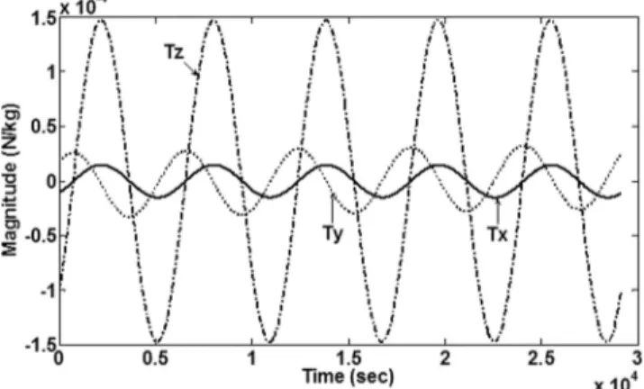
Figure 1 shows thrust accelerations in each axis during the rendezvous. The solid line represents the values of T_x, the dotted line represents the values of T_y, and the dash-dotted line represents the values of T_z. From (27) and (38), it is found that T_x and T_z are sinusoidal and periodic, whereas T_y slightly increases with oscillations. The total simulation time in Figs. 1—4 is the chief satellite’s five orbital periods. Fig. 2 shows the difference between the thrust accelerations obtained by (38) and (27) in this paper and those calculated by [14], which uses the HCW equations assuming no perturbations. They differ by about 1% in total thrust for the case. It is found that

the difference of the accelerations is changed as the inclination of reference orbit varies. The difference is maximized (2.3%) when i_ref= 0 or 180 deg. The relatively small difference in the accelerations occurs because the coefficients of the modified HCW equations differ only slightly from those of the HCW equations. Because the time average of the gradient of the J₂ potential is used, the orbital period of the reference orbit has been adjusted to match the period of the satellite, and the reference orbit’s ascending node is forced to move at the same speed as the ascending node of the satellite’s orbit. Fig. 3 shows the three-dimensional optimal trajectory in the LVLH frame during the rendezvous. The square and circle are used to show the initial and final relative position, respectively. The narrow line is a trajectory with the initial condition without consuming thrusts. The solid line represents the optimal trajectory, which is obtained from the analytic solutions ((4), (11), (12), and (29)). After five periods, the deputy successfully has a rendezvous with the chief. Fig. 4 shows the difference between position vectors when the linear dynamic model given in (1a)—(1c) is used; the position vector given in Fig. 3 is subtracted from that obtained when the thrust accelerations given by [14] have the same initial conditions. Because the homogeneous solutions are the same, this figure directly denotes the difference between the two particular solutions. The difference is getting larger, as expected. This indicates that the effect of the J₂ perturbation cannot be ignored. An important feature is that there is a large drift in the along-track (y) direction. This results from the particular solution of the along-track direction having a relatively large secular term, namely, the t3 _{term in I}

5(t) in (40). Physically, the J₂ effect invokes a small relative tangential velocity difference between the deputy and the chief satellites, and it is magnified with time. Although this feature captures the general behavior of the relative distance in the presence of the J₂ disturbance, the linear models in [14] and in this paper tend to underestimate the drift in the along-track direction. The initial conditions for the free-orbit ellipse cancel the drift in the linear model but not in the nonlinear model. Moreover, the nonlinear gravity, which is not incorporated in the linear model, amplifies the secular drift, yielding drifts in the radial and cross-track directions. To evaluate the underestimated amounts by either of the two linear models, numerical simulations are performed using the nonlinear model (~F_obl), including J₂ perturbations in ~ F_obl=_¡¹ r3~r¡ ¹J2R2e · 3Z r5 ˆk + μ 3 2r5¡ 15z2 2r7 ¶ ~r ¸ + ~T_ECI (42)

(13)

Fig. 1. Thrust accelerations in each axis for rendezvous maneuver with J₂perturbations during chief’s five orbital periods (deputy’s initial ½₀and Á are chosen to be 2000 m and 45 deg). Figure 3 shows three-dimensional optimal trajectory in LVLH

frame during rendezvous.

Fig. 2. Difference between thrust accelerations in Fig. 1 and those calculated by [14] with no J₂ perturbations.

where ~r = Xˆi + Yˆj + Z ˆk is the satellite position vector in the Earth-centered inertial (ECI) frame and ~T_ECI is the thrust acceleration obtained using the two linear models (HCW equations used in [14] and the linear dynamics model given here by (1a)—(1c)). The thrust acceleration can be analytically calculated in the LVLH coordinate using the results in this paper or in [14] and can be converted to the value in the ECI coordinate system. The nonlinear model gives the absolute motion of satellite in the ECI frame. The motion of satellite is then converted to the LVLH coordinate. To check the accuracy of our linear dynamic model and the linear dynamic model in [14], the nonlinear model of (42) and the two linear dynamic models are used to calculate the satellite motions without the thrust acceleration. The conditions of (41) are used as initial conditions for the simulations. Here, ½₀and ' are chosen to be 2000 m and 45 deg, respectively. For the initial orbital elements of the reference orbit, the semimajor axis is 7000 km; the mean eccentricity is 0; the inclination varies from 0 to 90 deg; the other elements are set to

Fig. 3. Three-dimensional optimal trajectory of rendezvous in LVLH frame when accelerations in Fig. 1 are applied with J₂

perturbations.

Fig. 4. Difference between position vectors in Fig. 3 obtained in this paper and position vectors obtained by thrust accelerations in

[14] for same rendezvous problem.

0. The satellite motions obtained from the nonlinear model are compared to those from the two linear models to check the accuracy of the two linear models with respect to the nonlinear model. The orbit of the satellite is numerically propagated for 12 h using the nonlinear model in an ECI frame with J₂perturbation, and then it is transformed into the LVLH frame.

Figure 5 demonstrates the root mean square (RMS) of the position differences between the two linear models and the nonlinear model after the simulation time of 12 h. The RMS values of each component are shown as the inclination of the chief satellite varies. As expected, the drift in the along-track direction (y-component) by both linear models is dominant for most inclinations of the satellite. The drift of the cross-track direction (z-component) in the HCW linear dynamic model cannot be ignored for lower inclinations, and it can reach its maximum as the inclination goes to 0 deg. For the rendezvous problem, the thrust acceleration is analytically calculated using our results or those of [14], and it is applied to the nonlinear dynamic model given by (42). As the inclination of the chief satellite varies, the numerical simulations are performed in the same initial conditions and final conditions used

(14)

TABLE I

Position Errors of Rendezvous Problem in Nonlinear Dynamic Model when Thrust Accelerations are used from this Paper (T_J2) and [14] (T_HCW)

½ (m) x-axis (m) y-axis (m) z-axis (m)

i (deg) T_J2 T_HCW T_J2 T_HCW T_J2 T_HCW T_J2 T_HCW 0.1 60.32 146.77 ¡21:40 ¡12:85 37.19 116.39 ¡42:40 ¡88:48 5 68.09 154.87 ¡21:09 ¡12:63 49.01 127.07 ¡42:29 ¡87:62 15 90.58 169.62 ¡20:03 ¡12:33 77.68 148.22 ¡42:06 ¡81:55 25 118.65 181.08 ¡18:49 ¡12:21 109.51 166.46 ¡41:73 ¡70:22 35 147.52 188.18 ¡16:65 ¡12:30 140.67 179.61 ¡41:18 ¡54:78 45 172.77 190.06 ¡14:73 ¡12:58 167.34 186.02 ¡40:37 ¡36:90 55 190.78 186.21 ¡12:98 ¡13:02 186.23 184.81 ¡39:34 ¡18:69 65 199.06 176.53 _¡11:60 _¡13:56 195.00 175.99 _¡38:28 _¡2:41 75 196.46 161.47 _¡10:75 _¡14:13 192.56 160.55 _¡37:47 9.76 85 183.34 142.08 _¡10:52 _¡14:66 179.23 140.39 _¡37:13 16.17 89.9 173.54 131.46 _¡10:66 _¡14:90 169.17 129.52 _¡37:19 16.90

Note: The error varies with respect to the inclination of the chief satellite. ½ is the total absolute error of the final position, and the x-, y-, and z-axes indicate the component in radial, along-track, and cross-track directions, respectively.

Fig. 5. Position errors of HCW linear model and linear dynamic model (in [8]) used in this paper are numerically analyzed using nonlinear dynamic model given in (42) without thrust acceleration. Vertical axis is RMS of position error for simulation time of 12 h,

and horizontal axis is inclination of chief satellite. ½ is total absolute error, and x-, y-, and z-axes note component in radial,

along-track, and cross-track directions, respectively.

for Figs. 1—4. The errors of final positions from the numerical simulations are compared in Table I.

The error varies with respect to the inclination of the chief satellite. In Table I, ½ is the total absolute error of final position, and the x-, y-, and z-axes indicate the component in radial, along-track, and cross-track directions, respectively. For an inclination of less than i_ref_{¼ 54:735 deg, the thrust acceleration} (T_J2) that we calculated gives smaller errors of the final position than those found when the thrust acceleration (T_HCW) calculated in [14] is used. The error of the final position by the thrust acceleration in this paper is reduced by up to 59% of the error

yielded by the thrust acceleration in [14] as the inclination of satellite approaches 0 deg. The reason for this phenomenon results from the linear dynamic model used to establish the thrust acceleration. As shown in Fig. 5, dynamic errors from the linear dynamic model used in this paper are less than the dynamic errors from the linear dynamic model used in [14] when the inclination is less than i_ref_¼ 54:735 deg. The J₂perturbations yield stronger effects near the bulge of Earth, which means small orbital inclinations. Hence, when the orbital inclination of the satellite is small, our dynamic model would be more accurate than the HCW dynamic model in [14]. Consequently, our dynamic model gives more accurate results in control simulation at small inclinations. However, the trend is reversed for the inclination larger than i_ref_{¼ 54:735 deg. Hence, it is} found that the accuracy of thrust acceleration depends on the accuracy of the linear dynamic model used to analytically calculate the thrust acceleration. The relative orbital dynamics in (1a)—(1c) under the J₂ disturbance used in this paper is different from that in the HCW equations used in [14]. Our relative orbital dynamics contains some parameters, such as s, c, q, and l, that are determined by the inclination i_ref and the radius r_ref of the reference orbit. When s=0, where s = (3J₂R2

e=8rref2 )(1 + 3 cos 2iref), the in-plane motion of the dynamics is the same as that of the HCW equations. Therefore, when i_ref_{¼ 54:735 or} 125.265 deg, which implies s = 0, the solutions of optimal trajectory using the two dynamics become the same. In addition, the solutions from the two dynamics have the largest differences when i_ref= 0 or 180 deg, which implies that s has the maximum value.

As a second simulation, the deputy satellite, which is initially placed in a free-orbit ellipse, resizes its configuration twice; that is, in (41), ½₀is chosen to be 2000 m at first and increases into 4000 m in the end. The phase angle Á is 45 deg for both the initial and

(15)

Fig. 6. Thrust accelerations in each axis for formation reconfiguration maneuver during chief’s five orbital periods. Figure 8 shows three-dimensional optimal trajectory in LVLH

frame during reconfiguration.

Fig. 7. Difference between thrust accelerations in Fig. 6 and those calculated by [14] with no J₂ perturbations.

the final conditions. For the formation reconfiguration, the initial conditions are x = 707:1 m, _x = 0:7615 m/s, y = 1414:2 m, _y =_{¡1:525 m/s, z = 1414:2 m, and} _z = 1:526 m/s; the final conditions are x = 1414:2 m, _x = 1:523 m/s, y = 2828:4 m, _y = ¡3:050 m/s, z = 2828:4 m, and _z = 3:053 m/s. The maneuver time is five periods of the reference orbit.

Figure 6 shows thrust accelerations in each axis during the maneuver. T_x and T_z are sinusoidal, but T_y slightly decreases with oscillations in this case because the sign of T₁ (or ¸₅) in (38) is positive. The total simulation time in the Figs. 6—9 is the chief satellite’s five orbital periods. Figure 7 shows the difference between the thrust accelerations determined from the analytic solutions in (38) and (27) here and those given by [14], which uses the HCW equations assuming no perturbations. They differ by about 5% in total thrust, and the difference grows smaller with respect to time for every axis. The difference of the accelerations is changed as the inclination of reference orbit varies. The difference is maximized (6.2%) when i_ref= 0 or 180 deg. Comparing the two frequencies in the thrust accelerations for each axis, we find that they differ slightly from each other, so

Fig. 8. Three-dimensional optimal trajectory of reconfiguration in LVLH frame when accelerations in Fig. 6 are applied with J₂

perturbations.

Fig. 9. Difference between position vectors in Fig. 8 obtained in this paper and position vectors obtained by thrust accelerations in

[14] for same reconfiguration problem.

Fig. 7 represents a “beat”-like phenomenon. Figure 8 shows the three-dimensional optimal trajectory in the LVLH frame during the resizing. The elements of the figure are as explained previously for Fig. 3. After the chief revolves five times, the deputy is placed at the final desired state. Figure 9 shows the difference between position vectors when the linear dynamic model given in (1a)—(1c) is used; the position vector given in Fig. 8 is subtracted from that obtained when the thrust accelerations given by [14] with the same initial conditions. The difference grows larger, which indicates that the effect of the J₂ perturbation cannot be ignored. As in Fig. 4, there is a secular drift in the along-track direction.

For the reconfiguration problem, the analytic thrust accelerations from the two linear dynamic models are applied to the nonlinear dynamic model of (42). The results of the numerical simulations are compared to the final positions of the reconfiguration problem, as shown in Table II. As with the rendezvous problem, for an inclination of less than i_ref_¼

54:735 deg, our calculated thrust acceleration gives smaller errors of the final position than those found when the thrust acceleration calculated in [14] is used. The error of the final position by the thrust acceleration in this paper is reduced by up to 25%

(16)

TABLE II

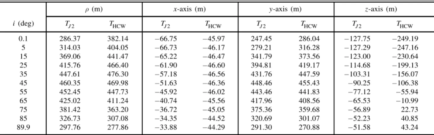
Position Errors of Reconfiguration Problem in Nonlinear Dynamic Model when Thrust Accelerations are used from this Paper (T_J2) and [14] (T_HCW)

½ (m) x-axis (m) y-axis (m) z-axis (m)

i (deg) T_J2 T_HCW T_J2 T_HCW T_J2 T_HCW T_J2 T_HCW 0.1 286.37 382.14 ¡66:75 ¡45:97 247.45 286.04 ¡127:75 ¡249:19 5 314.03 404.05 ¡66:73 ¡46:17 279.21 316.28 ¡127:29 ¡247:16 15 369.06 441.47 ¡65:22 ¡46:47 341.79 373.56 ¡123:00 ¡230:64 25 415.76 466.40 ¡61:90 ¡46:60 394.81 419.17 ¡114:68 ¡199:13 35 447.61 476.30 ¡57:18 ¡46:56 431.76 447.59 ¡103:31 ¡156:07 45 460.35 469.98 ¡51:63 ¡46:36 448.46 455.43 ¡90:25 ¡106:38 55 452.45 447.73 ¡45:92 ¡46:02 443.46 441.83 ¡77:12 ¡55:94 65 425.02 411.24 _¡40:74 _¡45:56 417.96 408.56 _¡65:53 _¡10:99 75 381.42 363.20 _¡36:72 _¡45:05 375.36 359.68 _¡56:89 22.73 85 326.73 307.08 _¡34:35 _¡44:52 320.69 301.07 _¡52:23 40.85 89.9 297.76 277.86 _¡33:88 _¡44:29 291.30 270.88 _¡51:58 43.24

Note: The error varies with respect to the inclination of the chief satellite. ½ is the total absolute error of the final position, and the x-, y-, and z-axes indicate the component in radial, along-track, and cross-track directions, respectively.

of the error yielded by the thrust acceleration in [14] as the inclination of the satellite approaches 0 deg. However, the trend is reversed for the inclination larger than i_ref_{¼ 54:735 deg. As mentioned for the} rendezvous problem, this phenomenon results from the approximations of linear dynamic models used to calculate the analytic thrust acceleration.

Our analytic solution is a modification of the solution given by [14] to adopt the J₂orbital perturbations, but it has some drawbacks because of the drawbacks of the modified dynamic model used to derive the solution. The main drawback is that the modified HCW equations presented by Schweighart and Sedwick [8] are sensitive to initial conditions. In the process of averaging the gradient of the J₂ disturbance over one period, some information within the orbital period is lost, so the appropriate initial conditions are mandatory, and several coefficients in the cross-track direction are obtained through spherical geometry. Our optimal solution is as simple as that given in [14]; it must be more accurate even in the presence of the J₂ potential disturbance when the inclination of satellites in formation flying is less than 54.735 deg. For the maneuvers treated in this study, the magnitude of the thrust accelerations is no larger than about 1:5_{£ 10}¡4N/kg. This order of magnitude is easily achieved by current engine technology. Thus, the results in this study can be utilized for the relative maneuvers. To extend the applications, it is challenging to evaluate analytic solutions for bounded thrust. This is beyond the scope of this study, and we plan to address this problem in a future study. VI. CONCLUSIONS

We derive novel closed-form solutions to the optimal reconfiguration of satellites flying in a formation under the J₂ perturbation. Our procedure to obtain the analytic solution is similar to that in [14]. However, we use a different dynamic model

to include the J₂ orbital perturbations and obtain an analytic solution that has been modified appropriately. The thrust accelerations are low level, continuous, and of variable magnitude. For the given initial and desired relative states of a satellite under the J₂ disturbance, we immediately generate an appropriate thrust acceleration and reconfiguration trajectory in a completely analytic method. With the analytic solution obtained in this paper, a reconfiguration controller can be easily designed to relocate the satellites into desired states even when the J₂disturbance cannot be ignored. The numerical simulations show the difference between our solution and those given in the previous research, assuming no perturbation. For an inclination of less than i_ref_{¼ 54:735 deg, the thrust} acceleration calculated in this paper gives smaller errors of the final position than those found when the thrust acceleration calculated in [14] is used. Thus, our solutions can be applied to any linear relative motions of a satellite with an inclination of less than i_ref_{¼ 54:735 deg to improve the results by including} the J₂perturbations. This analytic solution can be employed in preliminary analysis as a more practical tool, used as an initial approximation for finding an exact solution, and used as a base at early stages of space mission design.

REFERENCES

[1] Aoude, G. S., How, J. P., and Garcia, I. M.

Two-stage path planning approach for designing multiple spacecraft reconfiguration maneuvers.

In Proceedings of the 20th International Symposium on

Space Flight Dynamics, Annapolis, MD, Sept. 2007.

[2] Hill, G. W.

Researches in the lunar theory.

American Journal of Mathematics, 1, 1 (1878), 5—26.

[3] Clohessy, W. H. and Wiltshire, R. S.

Terminal guidance system for satellite rendezvous.

Journal of the Aerospace Sciences, 27, 8 (1960), 653—658,

(17)

[4] Sabol, C., Burns, R., and McLaughlin, C. A. Satellite formation flying design and evolution.

Journal of Spacecraft and Rockets, 38, 2 (2001), 270—278.

[5] Kechichian, J. A.

Motion in general elliptic orbit with respect to a dragging and processing coordinate frame.

Journal of the Astronautical Sciences, 46, 1 (1998), 25—45.

[6] Sedwick, R. J., Miller, D. W., and Kong, E. M. C. Mitigation of differential perturbations in clusters of formation flying satellites.

In Proceedings of the 9th AAS/AIAA Space Flight

Mechanics Meeting, AAS 99-124, Breckenridge, CO, Feb.

1999.

[7] Hamel, J-F. and de Lafontaine, J.

Linearized dynamics of formation flying spacecraft on a J₂-perturbed elliptical orbit.

Journal of Guidance, Control, and Dynamics, 30, 6 (2007),

1649—1658.

[8] Schweighart, S. A. and Sedwick, R. J.

High-fidelity linearized J₂model for satellite formation flight.

1073—1080. [9] Ross, I. M.

Linearized dynamics equations for spacecraft subject to J₂ perturbations.

657—659. [10] Lawden, D. F.

Optimal Trajectories for Space Navigation.

London: Butterworths, 1967, pp. 79—95. [11] Zanon, D. J. and Campbell, M. E.

Optimal planner for spacecraft formations in elliptical orbits.

161—171.

[12] Tillerson, M., Inalhan, G., and How, J. P.

Co-ordinate and control of distributed spacecraft systems using convex optimization techniques.

International Journal of Robust and Nonlinear Control, 12

(2002), 207—242.

[13] Vaddi, S. S., Alfriend, K. T., Vadali, S. R., and Sengupta, P. Formation establishment and reconfiguration using impulsive control.

262—268. [14] Palmer, P.

Optimal relocation of satellites flying in near-circular-orbit formations.

519—526. [15] Boas, M. L.

Mathematical Methods in the Physical Sciences (2nd ed.).

New York: Wiley, 1983, pp. 307—334. [16] Cho, H-C., Park, S-Y., Yoo, S-M., and Choi, K-H.

Analytical solution to optimal relocation of satellite formation flying in arbitrary elliptic orbits. In Proceedings of the 17th AAS/AIAA Space Flight

Mechanics Meeting, AAS 07-108, Sedona, AZ, Jan. 2007.

[17] Tschauner, J. and Hempel, P.

Rendezvous zu einemin elliptischer bahn umlaufenden ziel.

Acta Astronautica, 11, 2 (1965), 104—109, in German.

[18] Yamanaka, K. and Ankersen, F.

New state transition matrix for relative motion on an arbitrary elliptical orbit.

60—66.

[19] Scott, C. J. and Spencer, D. B.

Optimal reconfiguration of satellites in formation.

Journal of Spacecraft and Rockets, 44, 1 (2007), 230—239.

[20] Sharma, R., Sengupta, P., and Vadali, S. R.

Near-optimal feedback rendezvous in elliptic orbits accounting for nonlinear differential gravity.

1803—1813.

[21] Schaub, H. and Alfriend, K. T.

Impulse feedback control to establish specific mean orbit elements of spacecraft formations.

739—745. [22] Sengupta, P.

Satellite relative motion propagation and control in the presence of J₂perturbations.

M.S. thesis, Texas A&M University, College Station, 2003.

[23] Horneman, K.

Reconfiguration and maintenance of satellite formations in the presence of J₂perturbations.

M.S. thesis, University of Missouri—Columbia, 2003. [24] Yan, H. and Alfriend, K. T.

Approximate minimum energy control laws for low-thrust formation reconfiguration.

1182—1185.

[25] Mathews, J. and Walker, R. L.

Mathematical Methods of Physics (2nd ed.).

New York: Benjamin/Cummings Publishing, 1970, pp. 8—13.

[26] Palmer, P.

Reachability and optimal phasing for reconfiguration in near-circular orbit formations.

1542—1546.

[27] Vaddi, S. S., Vadali, S. R., and Alfriend, K. T. Formation flying: Accommodating nonlinearity and eccentric perturbations.