CIRPÉE
Centre interuniversitaire sur le risque, les politiques économiques et l’emploi
Cahier de recherche/Working Paper 07-04
Research Cycles
Yann Bramoullé Gilles Saint-Paul
Février/February 2007
_______________________
Bramoullé: Department of Economics, GREEN and CIRPÉE, Université Laval, Québec.
Saint-Paul: IDEI, GREMAQ, LEERNA, Université des Sciences Sociales, Toulouse; CEPR and IZA.
Abstract:
This paper studies the dynamics of fundamental research. We develop a simple model where researchers allocate their effort between improving existing fields and inventing new ones. A key assumption is that scientists derive utility from recognition from other scientists. We show that the economy can be either in a regime where new fields are constantly invented, and then converges to a steady state, or in a cyclical regime where periods of innovation alternate with periods of exploitation. We characterize the cyclical dynamics of the economy, show that indeterminacy may appear, and establish some comparative statics and welfare implications.
Keywords: Research dynamics, innovation cycles, indeterminacy JEL Classification: O39, C61
“my love of natural science (...) has been much aided by the am-bition to be esteemed by my fellow naturalists.” Darwin (1958).
1
Introduction
This paper studies the dynamics of fundamental research. We observe that periods of intense innovations are followed by periods of exploitation of ex-isting fields. We want to understand these dynamics and be able to study whether they are efficient from the point of view of social welfare.
A key aspect we are interested in is the credential one. Scientists derive utility from recognition from other scientists, which often takes the form of citations. In our model, the value derived by a scientist from a paper he has written is the sum of an “intrinsic” value of the paper, which depends on the field in which it is written and its order of appearance in that field, and a “citation premium” which depends on the number of subsequent papers written in that field.
We show that our model yields a rich set of results, both with respect to the cyclical dynamics of the allocation of the research effort and in terms of the comparative statics around the steady state, when it exists.
More specifically, we show that the economy can be either in a regime where new fields are constantly invented, and then converges to a steady state, or in a cyclical regime where periods of innovation alternate with peri-ods where one only exploits existing fields. Furthermore, these cycles are very irregular and the duration of a cycle is “unpredictable” from the duration of the previous cycle — i.e. related to it by a very nonlinear function.
Furthermoire, we are able to perform comparative statics in the conver-gence regime and show that a (i) higher citation premium raises the equi-librium rate of innovation, (ii) a mean-preserving spread in the distribution
of the value of new fields reduces the equilibrium rate of innovation and (iii) a larger citation premium makes researchers less risk-averse, in that it alleviates (and potentially reverses) that effect.
We introduce the distinction between extensive and intensive research to the study of scientific progress. Studies of technological changes have long stressed the difference between improvements of known processes and inno-vations leading to new products (e.g. Rosenberg (1972)). Similarly, it seems that some scientific contributions are pioneering and open up new avenues for future research, while others mainly refine or extend previous work. This distinction lies at the core of Kuhn (1970)’s influential theory of scientific evolution. In his view, science alternates between periods of normal sci-ence and scientific revolutions. Under normal scisci-ence, progress is gradual and builds up on past achievements. In contrast, scientific revolutions cor-respond to paradigm shifts during which scientists qualitatively change their focus and assumptions. Without necessarily adhering to Kuhn’s view, other observers have noted the importance of fads and fashions in science. Bron-fenbrenner (1966) gives an early account of fads in economics. Stephan and Levin (1991) discuss how scientific fashions might affect a scientist’s career. Sunstein (2001) relates academic fads to informational cascades.
This literature remains relatively undeveloped.2 We develop the first
formal model of the evolution of science that gives rise to innovation cycles and scientific fashions. We also explicitly account for the unique reward structure of science, by assuming that scientists care for recognition by their peers through citations of their work.3
In the literature on growth,4 several papers look at innovation cycles.
2Exceptions include Levin and Stephan (1991), Brock and Durlauf (1999), Goyal et al.
(2006), see also Stephan (1996) and the references therein.
3Scientists could also care for citations because of the financial gains they generate, see
e.g. Diamond (1986).
Jovanovic and Rob (1990) and Jovanovic and Nyarko (1996) build learning models. In Jovanovic and Rob (1990), an agent can explore a known or an unknown dimension of the technological space. Innovation cycles emerge for an intermediate range of the parameters. In Jovanovic and Nyarko (1996), the agent chooses between a known and a better, but unknown, technology. Permanent upgrading and growth can coexist with technological lock-in and stagnation. Matsuyama (1999) shows how innovation cycles can emerge in an endogenous growth model. Phases where investment is concentrated on old technologies alternate with phases with innovation. Innovation cycles emerge because of the temporary monopoly power enjoyed by innovators.
In contrast, the mechanism that drives our cycles is due to a multiplier effect, namely the fact that one unit of effort devoted to creating a new field today induces more than one unit of effort to exploit this field tomorrow.
Another novelty of our specification, relative to these papers, is the cita-tion premium.5 Through citations, payoffs from a scientist’s current choice
depend on the future evolution of science. This introduces a non-trivial dynamic linkage between current and future actions. We show that the ex-istence of innovation cycles does not depend on that of a citation premium, but that it affects their characteristics. In particular, a higher improvement phase tends to reduce the length of the improvement phase relative to the invention phase.
Note that our results could also potentially be applied to the analysis of commercial R & D, with our citation premium being reinterpreted as
which studies the incentive to innovate in one sector vs. another (See Acemoglu, 1998). The determinants of innovation in existing vs. new fields which we discuss here, however, are substantially different from the ones studied in that literature. The two approaches could be brought together, however, by assuming that exploiting existing fields uses dif-ferent factors of production than invention.
5Another difference is that the agent can make one search per period in Jovanovic
and Rob (1990) and Jovanovic and Nyarko (1996), while in our model research effort is continuous and allocated among different alternatives in every period.
the income derived by an innovator from the royalties paid by subsequent innovators building on his or her invention. The level of the citation premium can then be interpreted as the level of intellectual property6.
The rest of the paper is organized as follows. We introduce the model in section 2. We present our main result in section 3 and interpret it in section 4. We derive comparative statics in section 5 and comparative dynamics in section 6. We show that indeterminacy may appear in section 7, and establish some welfare results in section 8.
2
The model
We consider an infinite horizon model with discrete time. At each date t there is a continuum of existing fields of research, which we index by i. Each field is characterized by a stock of contributions (or ‘papers’) nt(i)at the end
of period t.
Papers are produced by researchers. Researchers live for two periods, hence we have an overlapping generation structure. In the first period of their life, researchers produce contributions. In the second period of their life, they enjoy the returns from their scientific “reputation”, which defines their utility function. A researcher’s scientific reputation is the sum of the contribution of each individual paper he or she has written. An individual paper written at date t in existing field i yields the following contribution to its author’s reputation:
vt(i) = ω(i)− β(ln nt(i)− ln ¯n) + θ(ln nt+1(i)− ln nt(i)).
This reputation is the sum of two terms. The first term, ω(i)−β(ln nt(i)−
ln ¯n), defines the intrinsic value of the paper. ω(i) is a field-specific constant
6Or, more generally, as the degree of appropriability of the returns to innovation
which represents the field’s value (or initial research potential) as a whole. The term β(ln nt(i)− ln ¯n), where β and ¯n are positive parameters, captures
the fact that there are decreasing returns to research: the larger the stock of knowledge in field i, the smaller the intrinsic value of additional contributions. The second term, θ(ln nt+1(i)− ln nt(i)), is the citation premium. It tells us
that the reputation obtained from papers written at t is greater, the greater the flow of further advances in the relevant field at t + 1. Underlying this formulation is the idea that papers come in a given order, and that new papers cite previous papers, thus enhancing their author’s reputation. Note that contemporaneous papers do not cite each other, so that what matters for citations is the log difference between the stock of papers written at the end of t + 1 and that at the end of t.
The total mass of researchers per generation is normalized to 1. Each researcher is endowed with ν units of time. He allocates his time optimally between writing papers in different fields. In addition to that, one may create new fields.7
When one writes the first paper in a new field, its potential ω(i) is drawn from some distribution, with pdf f (.), such that all moments exist. The realization of ω(i) is unknown when one decides to write the paper. At the end of the period when the new field is created, its advancement level is set at the minimal value ¯n. Therefore, one must wait one period before making further contributions to a new field.
We assume that one unit of time produces either 1 paper in an existing field or γ papers in a new field.
We make two technical assumptions that we need to be able to solve the model:
7Note that this distinction between fundamental and secondary innovation is different
from the one used by Aghion and Howitt (1996, 2000 ch. 6), who assume that secondary innovation results from learning by doing only.
Assumption A1 — If at date t, there is a strictly positive measure of new fields invented, then all fields invented before date t can no longer be re-searched from date t + 1 on.
This assumption is a useful simplification that avoids having to keep track of all the fields ever invented at any date t.8 Only the fields invented in the
last wave of innovation can be exploited at a given date.9
Assumption A2 — γ < 1.
This assumption states that inventing a new field requires more labor than writing a paper in an existingf field. It is a plausible, but merely technical assumption, required to prove the existence of an equilibrium for θ > 0.10
3
Equilibrium
In this section, we show the existence of an equilibrium, and the conditions under which it is cyclical as opposed to converging to a steady state. We provide a result for uniqueness in the case where θ = 0. We first discuss the equilibrium conditions of the model in the two regimes of interest. We then state the paper’s main result, whose proof is relegated to the Appendix. In the next section, we discuss its economic interpretation using a graphical il-lustration, confining ourselves to the θ = 0 case. We then work out numerical
8This assumption is consistent with Kuhn’s theory: “When it repudiates a paradigm,
a scientific community simultaneously renounces most of the books and articles in which that paradigm had been embodied”, Kuhn (1970). See also theorem 2 in Jovanonvic and Rob (1990) and the “no-recall” assumption of Jovanovic and Nyarko (1996).
9It is not necessary to make this assumption in the special case where θ = 0. In such
a case the value of inventing a new field is VN = γ ¯ω = γE(ω), which is also the lower
bound of the value of working on an existing field, since one could always produce new fields instead. Consequently, when new fields are invented, all previous fields reach their maximum advancement level, such that the value of the marginal paper is equal to VN;
they will not be exploited thereafter.
examples. Finally, we give a sketch of the proof when the citation premium is positive.
3.1
Equilibrium conditions
At any point in time, the economy may be in one of two regimes:
In Regime I, all the research input is allocated to improving existing fields. There exists a shadow value of time λt; a field is exploited if and only if the
first paper written in the current period has a value greater than λt, that is:
ω(i)− β(ln nt−1(i)− ln ¯n) + θ(ln nt+1(i)− ln nt−1(i)) > λt.
The number of papers written in such a field, at t, must satisfy
ω(i)− β(ln nt(i)− ln ¯n) + θ(ln nt+1(i)− ln nt(i)) = λt.
The equilibrium value of λt must adjust so that the total mass of papers
being written is equal to υ. Call s the last period where invention took place, and µs the mass of new fields invented at s. The evolution of one of these
fields will clearly be a sole function of its intrinsic value ω. Thus nt can be
written as a sole function of ω rather than the field’s specific index i. The preceding conditions are equivalent to
ω > (β + θ) ln nt−1(ω)− β ln ¯n − θ ln nt+1(ω) + λt, (1) and nt(ω) = ¯n β β+θn t+1(ω) θ β+θe ω−λt β+θ . (2)
The full employment condition can therefore be written as µs
Z
ω>(β+θ) ln nt−1(ω)−β ln ¯n−θ ln nt+1(ω)+λt
(nt(ω)− nt−1(ω))f (ω)dω = υ. (3)
Finally, the value of writing a new paper, denoted by Vt, must be lower
than that of working on an existing field: Vt< λt.
In Regime II, people exploit existing fields, and work on new fields as well. They must be indifferent between the two activities, so that one must have λt= Vt.An existing field is exploited if and only if
ω > (β + θ) ln nt−1(ω)− β ln ¯n − θ ln nt+1(ω) + Vt. (4)
Its advancement level then proceeds to
nt(ω) = ¯n β β+θn t+1(ω) θ β+θe ω−Vt β+θ .
Because of Assumption (A1), the existing fields will disappear at t+1 and be replaced by the mass µt of new fields, which will start with advancement
level ¯n at t + 1.Therefore, nt+1(ω) = nt(ω), since existing fields at t are no
longer exploited at t + 1. Substituting, the final advancement level is:
nt(ω) = ¯ne
ω−Vt
β , (5)
while (4) can be rewritten
ω > Vt+ β(ln nt−1(ω)− ln ¯n).
Note that this condition collapses to
ω > Vt (6)
if the economy was also in regime II at date t − 1, since the field must then have been invented at that date.
In regime II, the resource constraint states that total time devoted to existing fields cannot exceed υ :
µs
Z
ω>β(ln nt−1(ω)−ln ¯n)+Vt
The remaining time endowment must be devoted to new fields; this de-termines the mass of new fields invented at t :
µt= γ ∙ υ− µs Z ω>β(ln nt−1(ω)−ln ¯n)+Vt (nt(ω)− nt−1(ω))f (ω)dω ¸ .
Finally, in both regimes, the value of working in a new field Vt is
deter-mined as follows. Consider a researcher writing a paper in a new field with value ω. Then, nt(ω) = ¯n. If (1) holds at t + 1, which is equivalent to
ω > θ ln ¯n− θ ln nt+2(ω) + λt+1,
then the field will be active, and the inventor will benefit from citations. The value to the inventor is then given by
Vt(ω) = ω + θ(ln nt+1(ω)− ¯n) where nt+1(ω) = ¯n β β+θn t+2(ω) θ β+θe ω−λt+1 β+θ .
Otherwise, the field will not be active at t + 1, and the inventor just gets the intrinsic value of the first paper:
Vt(ω) = ω.
Thus, the value of working on a new field at t is given by:
Vt = γ ∙ ¯ ω + θ β + θ Z ω>λt+1−θ(ln nt+2(ω)−ln ¯n) (ω− λt+1+ θ(ln nt+2(ω)− ln ¯n)) f(ω)dω ¸ .
3.2
Existence, uniqueness, and cycles
We now state the central results of the paper. To do so, we need to introduce the following two functions:
Φ(y) = γ ∙ ¯ ω + θ β Z +∞ y (ω− y) f(ω)dω ¸ , (7)
and
I∗(y) = Z +∞
y
(eω−yβ − 1)f(ω)dω.
Most of the equilibrium conditions involving the value of a new field V can be stated in terms of the Φ function; for example, it can be easily shown that if the economy is in regime II in two consecutive periods t and t + 1, then Vt= Φ(Vt+1).As for I∗, it shows up whenever one is adding progresses
across exploited fields to get the associated total labor input. For example, if θ = 0 and fields are exploited for the first time, then the LHS of (3) is equal to µsnI¯ ∗(λ
t).
Both functions are continuous and decreasing. Since Φ(0) ≥ γ ¯ω and Φ(+∞) = γ ¯ω, Φ has a fixed point ¯V :
Φ( ¯V ) = ¯V . (8)
The paper’s main result can be stated as follows:
PROPOSITION 1 — Assume that the economy starts at t = 0 with an initial mass of fields µ−1, whose intrinsic value is distributed with f (), and whose initial advancement level is given by ¯n. Then:
(i) There exists an equilibrium path. (ii) If
I∗( ¯V ) > 1
γ ¯n, (9)
then any equilibrium is cyclical, i.e. periods in regime I alternate with periods in regime II. During periods in regime II, the mass of invented fields follows explosive oscillations, until the economy reverts to regime I. During periods in regime I, the set of exploited fields grows. The duration of a period in regime I cannot exceed γ ¯nI∗(γ ¯ω).
(iii) If
I∗( ¯V ) < 1 γ ¯n,
then there exists an equilibrium such that -the economy is in regime II from t = 0 on.
-the value of working in a new field is equal to ¯V at all dates.
-the mass of invented fields converges to its steady state value, given by ¯
µ = γν
1 + γ ¯nI∗( ¯V ),
by dampened oscillations.
(iv) If θ = 0, equilibrium is unique.11
PROOF — See Appendix.
4
Interpretation
4.1
Without citation premium
To analyze the reason behind cycles, let us focus on the simpler case where θ = 0. In the absence of a citation premium, inventors of new fields just get the intrinsic value of the field, ω, as a reward. Consequently, the value of a new field is pinned down and equal to V = γ ¯ω in any period.
Figure 1 plots the value of working in an existing field at any date t, λt,as
a function of the total input in existing fields; that defines the LL schedule. This curve is downward-sloping, because of decreasing returns, captured by the −β(ln nt(i)− ln ¯n) term in the utility function. For the same reason,
its position is lower, the higher the initial advancement level of those fields, nt−1(i). Finally, given that level, its position is higher, the greater the mass of available fields µs, since the same total research input is now associated
with a lower advancement level nt(i)in each field.
If, as is the case in Figure 1, that schedule intersects the horizontal line VV at λ = V, then the economy is in regime II. The horizontal distance AB
determines the labor input into new fields, and hence the mass of fields being invented.
If that is not the case, then the economy must be in regime I, and equilib-rium determination is illustrated in Figure 2. At date t, all researchers work in existing fields. Advancement in these fields generate a downward shift in LL, and the intercept of the LL schedule for the next period must be equal to λt — which simply means that the value of the first marginal paper at t + 1
in a given field is equal to the value of the last paper written in that field at t. The process continues until the LL schedule cuts the VV schedule, in which case one is back to regime II (at t + 2 in the case of Figure 2). This must happen in finite time, otherwise decreasing returns would eventually drive VV below the λ = 0 line. Note that the λts fall during the regime I
period. That is the reason why the set of fields being exploited grows during that phase.12
What happens, next, in regime II? At each date, a given mass of fields is invented. The greater that mass, the greater the value of exploiting these fields next period (i.e. LL shifts up). On average, one field invented at date t, with a quality distribution f (ω), triggers an amount ¯nI∗(V ) of research input devoted to exploiting that field at date t + 1. That reduces the amount of time devoted to innovation: the greater the mass of fields invented today, the lower the mass of fields invented tomorrow. The evolution of µt,the mass
of fields invented at t, evolves according to
µt= γ(υ− µt−1nI¯ ∗(V )). (10)
If these dynamics are stable (¯nI∗(V ) < 1, Figure 3), then the economy
converges to a steady state. Otherwise, (¯nI∗(V ) > 1,Figure 4), the economy
12Because of assumption A1, a field exploited during that phase must have been invented
in the last period in regime II before the regime I phase. It enters regime I with an initial advancement level equal to ¯n. Using (1) with θ = 0, it will therefore be exploited as soon as ω > λt. Because the λs are falling, it will continue to be exploited until the economy
cannot remain in regime II forever: it will revert to regime I. As regime I itself cannot last forever, the two regimes must prevail alternatively.
The instability condition ¯nI∗(V ) > 1 simply means that a unit of labor employed in inventing a new field today attracts more than one unit of labor into exploiting that field tomorrow. That in turn reduces the amount of labor inventing new fields tomorrow more than one for one, thus generating the explosive oscillatory dynamics and the subsequent exit from regime II. The greater the quantity I∗(V ), the more invented fields are attractive, and the more likely it is that cycles arise.
4.2
Constructing an equilibrium
Constructing an equilibrium turns out to be easy in the θ = 0 case. Consider Regime I. At any date, there are two kind of fields: those who are exploited, and those who have never been exploited since their invention. The latter are such that ω ≤ λt have an advancement level equal to ¯n; the former, such
that ω > λt,reach an advancement level equal to nt(ω) = ¯ne
ω−λt
β .At t+1, all these fields are exploited, plus a mass of extra fields such that λt > ω > λt+1.
The research input into existing fields at date t + 1 is therefore equal to
υAt+1 = µs Z ω>λt+1 (nt+1(ω)− nt(ω))f (ω)dω = µs Z λt>ω>λt+1 (¯neω−λtβ − ¯n)f(ω)dω + µ s Z ω>λt (¯ne ω−λt+1 β − ¯ne ω−λt β )f (ω)dω = ¯nµs(I∗(λt+1)− I∗(λt)).
In the first period of regime I, t = s + 1, no field has been exploited and the equation boils down to
υAs+1= ¯nµsI∗(λs+1).
after regime I, one must have λT = V = γ ¯ω, and 0 ≤ υAT < υ. Therefore, it
must be that
(i) λt = I∗−1((t− s)nµ¯ν
s).
(ii) The duration of the regime I phase is entirely pinned down by the condition I∗−1((T − s) ν ¯ nµs)≤ V < I ∗−1((T − 1 − s) ν ¯ nµs), i.e. T − s − 1 = INT (I∗(V )nµ¯ s ν ). (11)
Note that one may have T = s + 1, in which case there is no regime I phase. This happens if and only if
I∗−1( ν ¯
nµs)≤ V. (12)
(iii) The economy enters regime II with an initial measure of new fields given by
µT = γ(υ− υAt)
= γ(υ− ¯nµs(I∗(V )− I∗(λT −1))) = γυ(1− DEC(I∗(V )nµ¯ s
υ )). (13)
Therefore, given an initial measure of invented fields at s, we can construct a unique, possibly empty, phase in regime I, and compute its length and the initial measure of invented fields in the first period T of the subsequent regime II phase.
The regime II phase is then constructed by mechanically applying (10). The economy asymptotically converges to the steady state if ¯nI∗(V ) < 1;
otherwise, it remains in regime II until date s0 such that
µs0nI¯ ∗(V ) > υ (14)
This gives the measure of invented fields available for the next regime I phase. One can then iterate the procedure. Note that s0 is determined uniquely: on
the one hand, the economy cannot remain in regime II after the first date which satisfies (14), as µs0+1 would then be negative. On the other hand, if
one picks up a date prior to s0 for the transition to regime I, it would satisfy (12), thus leading to an empty regime I phase, which would not change the equilibrium.
It should be noted that equation (13), which related the mass of invented fields after a phase in regime I to the mass of invented fields before that phase, is discontinuous and highly non linear. Thus we expect cycles to be irregular: the characteristics of a cycle, such as the time spent in each regime and the mass of invented fields, are almost “unpredictable” from the characteristics of the preceding cycle.13
4.3
Numerical illustration
In this section we provide some simulations in order to get a better idea of the irregular nature of the innovation cycles. We assume that the quality of a field ω is drawn from a uniform distribution over [0, ωu], implying ¯ω = ωu/2.
13A similar nonlinearity applies to the mass of invented fields at the end of phase II, and
the duration of phase II, as a function of the initial mass of invented fields µT. Solving for (10) yields µt+1= γν 1 + γ ¯nI∗ + µ µT− γν 1 + γ ¯nI∗ ¶ (−γ¯nI∗)(t−T ). One has to distinguish between two cases.
If µT >1+γ ¯γνnI∗, then s0− T must be even, and one must have
s0 = T + 2IN T Ãln γν µT (µc)+1(1+γnI∗)−γν 2 ln(γ ¯nI∗) + 1 2 ! . If µT <1+γ ¯γνnI∗, then s0= 2IN T Ãln γν µT (µc)+1(1+γnI∗)−γν 2 ln(γ ¯nI∗) ! + 1.
As the initial measure µT changes, the duration of phase II will jump, and so will µs0. Therefore, we also have discontinuities in the function which related µs0 to µT.
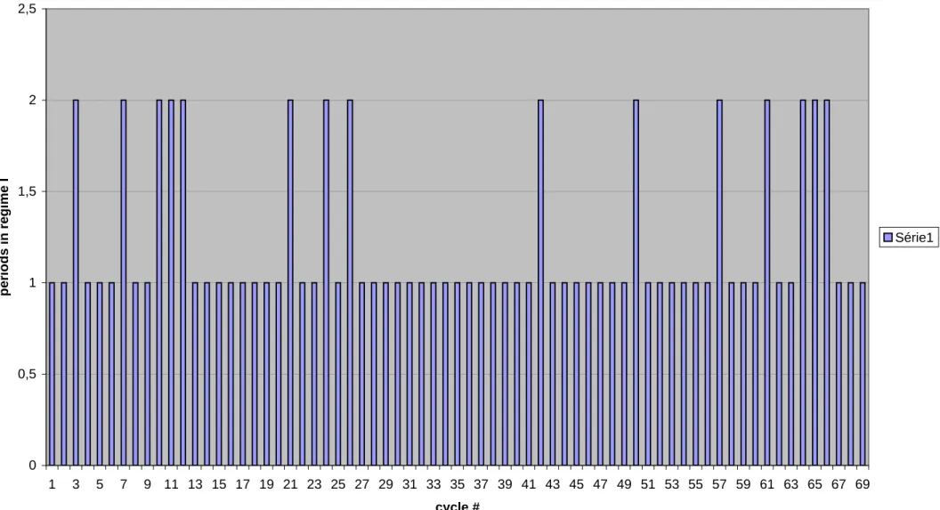
Figures 5 to 10 report the simulation results for the following set of pa-rameters: ¯n = 2; ωu = 1; β = 0.3; γ = 0.7; ν = 1. The initial measure of
existing fields was taken as µc= 1.
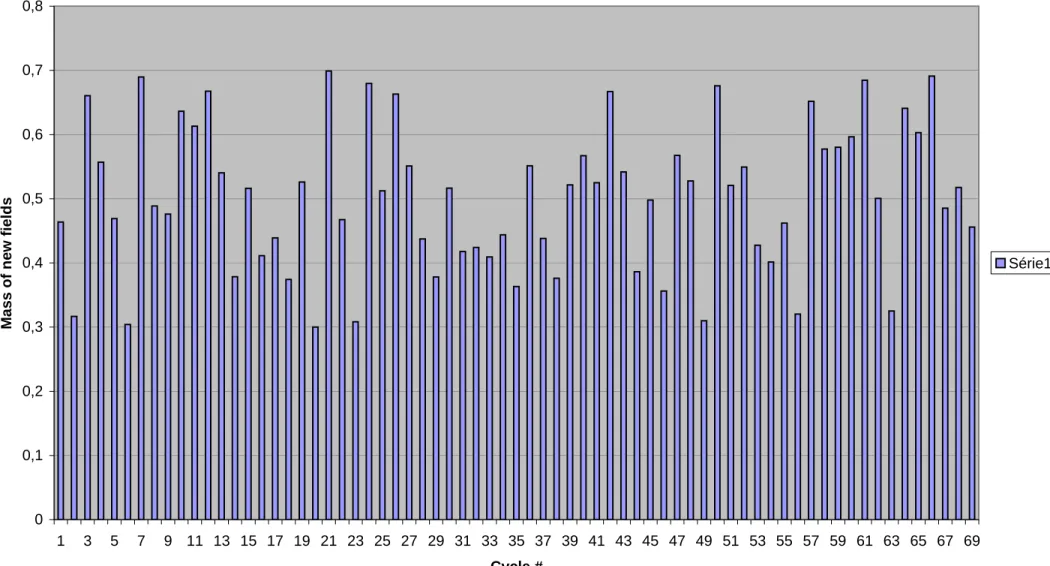
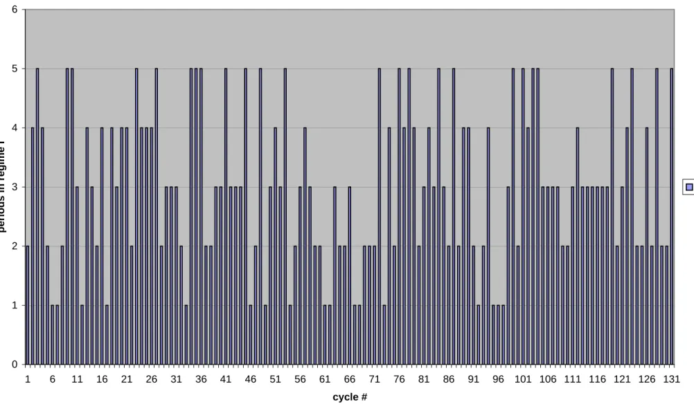
It is easy to show that (9) holds in this case, so that the equilibrium must be cyclical. The simulation shows that the economy follows cycles that are irregular, both in the duration spent in regime I and the duration spent in regime II. The time spent in regime I oscillates between 1 and 2 periods (Fig. 5), while time spent in regime II oscillates between 1 and up to 6 periods (Fig. 8)14. There are also chaotic oscillations in the stock of new
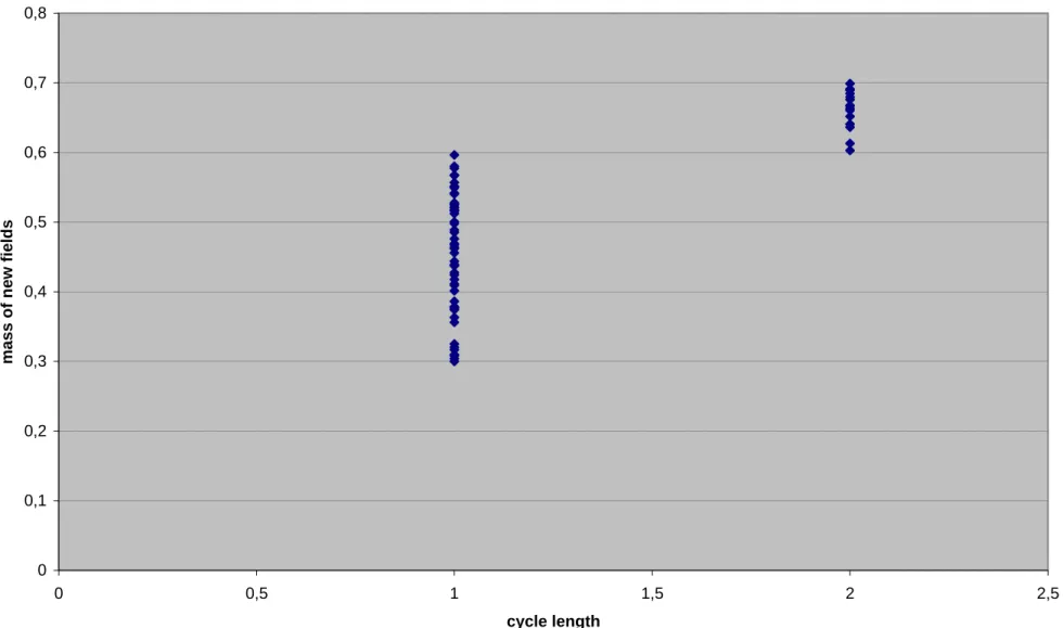
fields available for exploration at the beginning of each regime I phase (Figure 6). Furthermore, as (11) predicts, there is a tight connection between that initial stock and the length of the time spent in period 1 (Fig. 7); the regime I cycle lasts for 2 periods if the initial stock of knowledge is >≈ 0.6, and for 1 period otherwise.
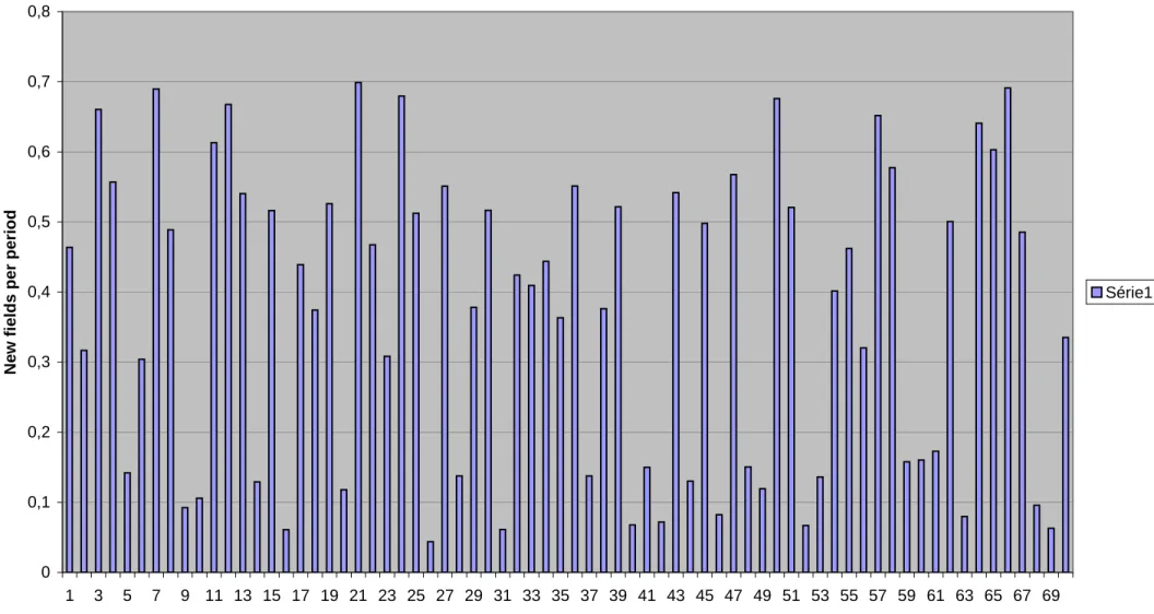
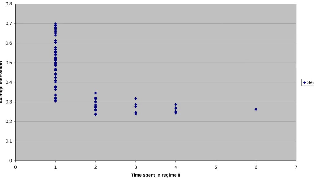
Figure 9 reports the average rate of innovation during the time spent in regime II. We see that it exhibits irregular fluctuations. We also see (Figure 10), that cycles where a longer time is spent in regime II, have a lower rate of innovation. Intuitively, if a large number of researchers produce new fields, it is more likely that the economy reverts to regime I in the following period in order to exploit the potential of these new fields15.
Relative to that benchmark simulation, we can perform some exercices. Figures 11 and 12 report the structure of cycles when we reduce the decreas-ing returns parameter from β = 0.3 to β = 0.2.16 We see that overall, the
14These figures report the 70 first cycles after the initial one.
15Another interesting property of that simulation, is that cycles where regime I lasts for
two periods, are such that the economy only spends 1 period in regime II. The explanation could be as follows: at the end of such cycles, fields are quite exhausted, and the value of working in new fields in regime II is quite high. Thus a large mass of innovation will take place during a short period of time, after which people revert to exploiting the new fields. However, this explanation is incomplete, since longer cycles are also those with a higher total initial potential. And that regularity is not robust to parameter changes.
economy spends more time in regime I and less time in regime II. In a cycle, regime I last between 1 and 5 periods, although that is quite often just 1 period, and regime II typically does not exceed 2 periods, although there are very rare occurences of cycles where the economy spends 3 periods in regime II.
In fact, while there is a maximum duration for the regime I phase, if the dynamics are truly chaotic one will have (very rare) regime II phases of arbitrary length. The reason is that the initial values of µ will span all the [0, γυ] interval, becoming sometimes arbitrarily close to the unstable steady state value ¯µ.
4.4
With citation premium
Two main difficulties arise when trying to extend the previous analysis to the case θ > 0. First, current exploitation of an existing field now depends on the future evolution of the field. Thus, nt(ω) depends on λt and nt+1(ω)
in eq. (2). And second, the value of writing a paper in a new field Vt will
generally vary with t.
In the Appendix, we show that the first issue can be addressed by back-ward induction from the last period of exploitation. Consider fields being exploited in a regime I episode, lasting from s + 1 to T − 1. Their exploita-tion ends at T , the first new period in regime II. At T , there are no more future citations for these fields, hence nT(ω) only depends on VT. This
de-termines the citation premium at T − 1 and nT −1(ω). Reasoning backward,
we show that the analysis for θ = 0 can be replicated through an appropri-ate change of variable on the shadow value of time λt. In the end, research
dynamics in regime I episodes only depend on two factors: the mass of fields originally available, µs+1, and the value of invention at the end, VT.
given by
T − s − 1 = INT (I∗(VT)
¯ nµs
ν ) while the mass of new fields invented at T is
µT = γυ(1− DEC(I∗(VT)
¯ nµs
υ ))
Next, we describe how the value of writing a paper in a new field, Vt,
evolves. This evolution differs within regimes and at regime transitions. Within regime I, changes in Vtdo not matter, as new fields are never invented.
Within regime II, it is easy to see that Vt= Φ(Vt+1). The final, key equation
is provided by the transition from regime II to regime I. Let s be a last period in regime II. The citation premium for new fields invented at s depend on the extent of their exploitation at s + 1, the first period of the new regime I phase. In turn, this mainly depends on the mass of new fields invented at s, µs. More precisely, we show in Appendix that:
Vs= Φ(I∗−1(
ν µsn¯))
Finally, we show that an equilibrium indeed exists. The proof is com-plicated by the fact that the function describing the evolution of µ is not continuous, nor contracting. We carefully construct sequences avoiding the discontinuities.
We are now in a position to analyze how the parameters of interest affect the equilibrium. We do it in two steps: first, we look at the case where (9) does not hold, and perform local comparative statics around the steady state. Second, we consider how the structure of cycles is affected by the model parameters when (9) holds.
5
Comparative statics
In this section, we perform local comparative statics around a regime II steady state. In particular, we are interested in how the equilibrium level of
invention, ¯µ, is affected by
• The citation premium θ,
• The distribution of field quality f(ω); in particular: how does the risk-iness of invention, measured by the variance of f (.), affect the equilib-rium allocation of effort between innovation and exploitation?
• The strength of decreasing returns β.
5.1
The effect of the citation premium
Equation (7) clearly implies that ¯V is an increasing function of θ. Further-more, one can straightforwardly check that dI∗/d ¯V < 0.Hence, d¯µ/d ¯V > 0.
Consequently,
PROPOSITION 2 — More research input is devoted to new fields, the higher the citation premium θ.
This result is not totally obvious. In principle, the citation premium increases incentives to work both in new fields and in existing fields. How-ever, in this equilibrium, existing fields are only exploited during one period; thus one earns no citation premium on them. An increase in θ thus clearly increases the value of working on new fields.
5.2
The role of research uncertainty
Next, we look at the role of uncertainty in research; we want to know how the variance of ω — or any mean-preserving spread parameter denoted by σ — affects the arbitrage between working in new fields vs. existing fields. As we shall see, option values intervene in two conflicting ways.
We first note that I∗(V )can be written as E(z(ω)), where z(ω) = max(eω(i)β−V− 1, 0) is a convex function of ω(i). By Jensen’s inequality, a mean-preserving
spread in the distribution of ω raises I∗(V ) for any given V. If V were to
remain unchanged, or move by only a little, µ would actually fall: more research uncertainty reduces the incentives to work in new fields.
If θ = 0, it is actually true that ¯V does not change in response to a mean-preserving change in the distribution of ω, for it is equal to γ ¯ω. Similarly, eq. (7) implies that for θ arbitrarily small the change in ¯V can be made arbitrarily small. Therefore:
PROPOSITION 3 — For θ small enough a mean-preserving spread in the distribution of ω reduces µ∞.
∂µ∞ ∂σ < 0.
Uncertainty increases the value of existing fields because one can select those of them with the highest potential. A greater variance of ω means that it is more valuable to work in the top field, while the value of working in the bottom fields is unchanged, because these fields are abandoned anyway. In contrast, the value of writing the first paper in an unknown field is increased is the field turns out to be good, but reduced if it turns out to be bad — if θ is small, then that value will roughly equal ω(i), regardless of the fate of the field after its invention. Hence greater uncertainty increases the value to work in known fields relative to unknown, new fields.
Against that logic, runs the fact that uncertainty increases the value of new fields, because of the citation premium. That is apparent from (7): a mean-preserving spread in ω increases its RHS. The option value of working in an existing field only if it is good enough also affects the value of working in new fields through the citation premium. When uncertainty goes up, researchers gain from their good ideas being cited more, but do not lose from their bad, uncited ideas, being cited less. In other words, the higher the citation premium, the less risk-averse the researchers.
PROPOSITION 4 — A mean preserving spread in ω increases ¯V : ∂ ¯V
∂σ > 0.
The effect is larger, the larger the citation premium: ∂2V¯
∂σ∂θ > 0.
Consequently, the larger the citation premium, the lower the negative ef-fect of uncertainty on the research input into new fields:
∂2µ ∞
∂θ∂σ > 0.
An interesting question is: can the reduction in risk aversion induced by the citation premium be so strong as to overturn the direct effect of uncertainty, so that one would have ∂µ∞
∂σ > 0? 17
5.3
The role of decreasing returns
A similar trade-off appears regarding the effect of β. It is easy to see that I∗(V )is a decreasing function of β. Thus, when θ = 0 or θ is small enough, µ
increases when β increases. Since existing fields lose their value more quickly, while the rewards from invention are (almost) unchanged, researchers devote more time to invention. As with uncertainty, an opposite effect comes into play through the citation premium. Observe that ¯V is decreasing in β when θ > 0. The citation premium is lower since with a higher β fields are being less exploited. Consequently, the value of writing a paper in a new field is lower (they will be cited less), which tends to counteract the first effect.
17We ran simulations, not shown here, with uniform distributions for ω. In these
6
Comparative dynamics
Given the highly nonlinear nature of our cycles, it is difficult to establish com-parative dynamics results. However, Proposition 5 establishes some results about the impact of the citation premium on the likelihood and structure of cycles. Typically, the casual idea that a greater citation premium makes “fads” more important and therefore cycles more likely, is not supported by the model. The reason is that the value of new fields goes up with the citation premium, which reduces the attractivity of existing fields, thus making it less likely that instability arises in (10). As the next section shows, however, a larger citation premium makes fads more likely in an indeterminacy sense.
PROPOSITION 5 — (i) The equilibrium is less likely to be cyclical, the greater θ.
(ii) Conditional on the initial mass of invented fields, the economy spends less time in the regime I phase for θ > 0 than for θ = 0. Furthermore, if the amount of time spent in regime I is the same, then more invention takes place at the beginning of the subsequent regime II phase, if θ > 0.
PROOF — See Appendix.
7
Indeterminacy and “sunspots”
The greater θ, the more expectations about future citations have a strong effect on the decision to work on a given field. By analogy with the literature on indeterminacy, we can speculate that there are multiple equilibria for θ large enough. That is actually the case. The following result shows that there is local indeterminacy around the regime II steady state for large enough values of θ.
PROPOSITION 6 — Assume γθ β (1− F ( ¯V )) > 1 and I∗( ¯V ) < 1 γ ¯n.
Then there exists a continuum of equilibria indexed by any initial value V0 = ¯V + vt, for vt sufficiently small.
PROOF — See Appendix.
This indeterminacy affects the value of invention. If scientists think that opening new fields brings a higher payoff, they devote more effort to inven-tion. The mass of papers in new fields is higher. This increases subsequent research in the better of these new fields. The citation premium originally associated to the new fields is thus effectively larger, which confirms the orig-inal expectation. In short, expecting invention to bring a high payoff can be a self-fulfilling prophecy.
8
Some welfare results
Due to the complexity of our model, it is not easy to make a thorough comparison between the equilibrium and the social optimum. However, it is possible to compare the steady state in regime II to its equivalent for the social planner. That is what we do in this section.
In order to perform a welfare analysis, a criterion is needed. There are many options since our model only specifies the value of innovation to re-searchers. An ample literature discusses the appropriability problems asso-ciated with research. Here we want to use our model to focus on only one market failure, which is that the stock of knowledge created by researchers
is durable and will benefit future generations beyond their lifetime. We then show that absent a citation premium the value of a new field in the equilib-rium steady state is lower than at the optimum steady state, and that an optimal “pigovian” citation premium can be introduced so as to induce the socially optimal level of fundamental. We provide a formula for computing this citation premium.
The social welfare function we use is as follows. At each date t there is a stock of knowledge Kt, which grows because of the introduction of new
fields and because of improvements in existing fields. We assume that the increase in the stock of knowledge is equal to the intrinsic value of all papers written at date t. Thus, the intrinsic value perceived by each researcher captures well their contribution to the knowledge stock. Researchers only fail to internalize the fact that their contribution increases the stock of knowledge forever. They get rewards from the flow of ideas they produce while society gets rewards from the stock of ideas.
We capture that with an intertemporal social welfare function given by
SW = +∞ X t=0 Kt (1 + φ)t,
where Kt is the stock of knowledge at t and φ the social discount rate, which
can conveniently be interpreted as an inverse measure of the weight put on future generations. The evolution of the knowledge stock is then given by, in regime II, Kt = Kt−1+µt Z ωf (ω)dω+µt−1 Z ω ÃZ nt(ω) ¯ n (ω− β(ln z − ln ¯n))dz ! f (ω)dω.
The first integral is the initial value of the fields invented at date t. The second integral is the contribution of the improvements made during t to the fields invented at t−1. Note that we integrate the marginal contribution of all papers ranked between ¯nand nt.This guarantees that researchers internalize
the congestion externality they exert upon others by moving, through their contribution, the state of the field down the marginal value curve. In other words, the intrinsic value of writing a paper in a field with potential ω is equal to its marginal effect on K, (ω − β(ln nt− ln ¯n)).
This equation may be rewritten
Kt= Kt−1+ µtω + µ¯ t−1
Z
ω
((ω + β) (nt(ω)− ¯n) − βnt(ln nt− ln ¯n))f(ω)dω.
(15) It can easily be shown that, as in the equilibrium, given the fraction of researchers who work in new fields, it is optimal to allocate the others so as to equate their intrinsic marginal value across active fields. Otherwise, one could reallocate the research effort across existing fields to get a higher value of the last term in (15). Consequently, at each date there exists a critical field ω∗
t such that nt(ω) = ¯nfor ω < ω∗t and nt(ω) = ¯ne
ω−ω∗t
β for ω ≥ ω∗
t. In steady
state, ω∗t will be constant through time. Using this property, the evolution
equation for knowledge can be rewritten as
Kt= Kt−1+ µtω + µ¯ t−1Γ(ω∗t), with Γ(ω∗) = ¯n Z +∞ ω∗ h (β + ω∗) eω−ω∗β − (β + ω) i f (ω)dω.
The social planner’s problem can be rewritten recursively by introducing the value function
V (µt−1, Kt−1) = max(Kt+
1
1 + φV (µt, Kt)).
Maximization takes place with respect to xt, the fraction of research
al-located to new fields. We thus have
while the resource constraint allows to compute ω∗
t as a function of x.
Ag-gregating the number of papers written in existing fields, we get
υ(1− x) = µt−1nI¯ ∗(ω∗t). (17)
PROPOSITION 7 — The steady-state, welfare maximizing value of ω∗ t is
determined by the following equation:
ω∗ = Ψ(ω∗),
where Ψ(.) is a decreasing function defined by
Ψ(ω∗) = γ ¯ω + nγ¯ 1 + φ
Z +∞
ω∗
∆(ω− ω∗)f (ω)dω, (18)
and where ∆(.) is a positive, increasing, convex function defined by ∆(x) = β(ex/β− 1) − x.
PROOF — See Appendix.
The critical level ω∗is the social opportunity cost of working in an existing field rather than a new field. Its equivalent in the analysis of the equilibrium is Vt,which is equal to ¯V, the fixed point of Φ in the equilibrium. Furthermore,
(5) and (6) show that a market economy will allocate employment across existing fields in exactly the same way as the social optimum if ¯V = ω∗.
Since the resource constraints (16) and (17) are the same in the equilibrium case and the optimum case, all that is needed to compare the equilibrium with the optimum is to compare the fixed point of Φ with that of Ψ. If they coincide, then the equilibrium steady state is identical to the social optimum steady state. Confronting (7) with (18) we then get that the two fixed points coincide provided the citation premium is equal to
θ∗ = nβ¯ 1 + φ R+∞ ω∗ ∆(ω− ω∗)f (ω)dω R+∞ ω∗ (ω− ω∗)f (ω)dω .
This citation premium goes down with φ, which means that it must be higher when the social planner cares more about future generations.18 That
is because the social planner puts more weight on subsequent improvements of a new field, the lower φ. The value of these subsequent improvements— which raises the value of a new field beyond its contemporaneous effect ¯ω— is internalized by the inventor only through the citation premium. Thus it must go up when φ goes down.
9
Conclusion
This paper has developed a simple model of the allocation of effort between fundamental research, which invents new fields, and applied research, which improves existing fields. Despite the model’s simplicity, our results are quite rich.
We were able to characterize the cyclical dynamics of the economy and derive a necessary and sufficient condition for cycles to arise. We have shown that indeterminacy may also appear, and that the citation premium makes the equilibrium less cyclical, but at the same time makes indeterminacy more likely.
We have also established some comparative statics for a steady-state in regime II, and to compare this steady state to the welfare optimum. We were able to highlight the role of the option value in determining the optimal and equilibrium allocation of research between the two activities.
18To see this, simply rewrite (8) as ¯V = Φ( ¯V ; θ), Φ0
1 < 0, Φ02 > 0, and (18) as ω∗ =
Ψ(ω∗, φ), Ψ0
1< 0, Ψ02< 0. The welfare maximizing value of θ, θ∗, is the unique solution to
10
Appendix:
10.1
Proof of proposition 1
λt is the shadow cost of a paper at t. Clearly one must have λt > γ ¯ω, which
is a lower bound for Vt, the value of inventing a new field.
At date t, a field i is exploited if and only if
ω(i)− β(ln nt−1(i)− ln ¯n) + θ(ln nt+1(i)− ln nt−1(i)) < λt,
in which case nt is determined by
ω(i)− β(ln nt(i)− ln ¯n) + θ(ln nt+1(i)− ln nt(i)) = λt.
A. One cannot forever remain in regime I
As if the θ = 0 case, we first prove that one cannot stay forever in regime I. We do so by contradiction.
Assume the economy is always in regime I from t on. Call µ the total mass of existing fields, indexed by i, and dF (i) their density. Assume a field is exploited at t. Then
ω(i)− β(ln nt(i)− ln ¯n) + θ(ln nt+1(i)− ln nt(i)) = λt> γ ¯ω;therefore,
ln nt+1(i)≥ β + θ θ ln nt(i) + γ ¯ω θ − ω(i) θ − β ln ¯n θ . A sufficient condition for nt+1(i) > nt(i) is therefore
nt(i) > ¯ne
ω(i)−γ ¯ω
β = k(i) (19)
. Hence, if a field is exploited at t and satisfies (19), then it will be exploited at t + 1. Since nt+1(i) in turn also satisfies (19), one has nt+2(i) > nt+1(i),
and so on. Therefore:
If a field satisfies (19) and is exploited at t, i.e. nt(i) > nt−1(i),then it is
Assume that at date t there is a set Λ with strictly positive measure of active fields such that (19) holds. Then, for each of these fields, nt+s+1(i) =
nt+s(i) ³ nt+s(i) k(i) ´β θ
.The quantity nt+s+1(i)−nt+s(i)is growing without bounds,
which contradicts the requirement that µRΛ(nt+s+1(i)− nt+s(i))dF (i) ≤ ν.
Consequently, such a set cannot exist. Let then Λt be the set of all active
fields at t. It must be that (19) is violated almost everywhere over Λt. Let
κt(i) = max(k(i)− nt(i), 0)≥ 0. We have that
Z Λt nt(i)dF (i) = Z Λt nt−1(i)dF (i) + ν µ Furthermore, as nt−1(i) < nt(i) < k(i)almost everywhere:
Z
Λt
κt(i)dF (i) =
Z
Λt
(k(i)− nt(i))dF (i)
= Z
Λt
(k(i)− nt−1(i))dF (i)− ν µ = Z Λt κt−1(i)dF (i)− ν µ.
On the other hand, nt(i) = nt−1(i) for i /∈ Λt, implying κt(i) = κt−1(i).
Therefore: Z Ω κt(i)dF (i) = Z Ω κt−1(i)dF (i)− ν µ.
We have constructed a sequence of positive functions whose integral even-tually becomes negative, which is a contradiction.
B. Characterizing dynamics in regime I
Let then T be the date when regime I ends: at date T one is in regime II. Let VT be the value of working in a new field at T. By assumption, all fields
invented prior to T are obsolete after T + 1. Hence T must be the last period when fields active during the regime I phase are exploited. An existing field is active at T iff
ω(i)− β(ln nT −1 − ln ¯n) > VT,
in which case nT is determined by
ω(i)− β(ln nT − ln ¯n) = VT.
Consider now a date t < T in the regime I phase. Denoting by λt the
shadow cost of a paper, a field is active iff
ω(i)− β(ln nt−1(i)− ln ¯n) + θ(ln nt+1(i)− ln nt−1) > λt
In which case
ω(i)− β(ln nt(i)− ln ¯n) + θ(ln nt+1(i)− ln nt(i)) = λt.
We now construct a sequence ˆλt such that the following property holds:
PROPERTY P1 — A field is active iff ω(i) − β(ln nt−1− ln ¯n) > ˆλt, in
which case ω(i) − β(ln nt− ln ¯n)) = ˆλt.
The sequence is constructed by backward induction, starting from t = T. We clearly can pick ˆλT = VT.Now, assume P1 holds for t0 > t.
Assume λt> ˆλt+1. Then all active fields at t must also be active at t + 1.
To prove so, suppose there is a field i active at t and inactive at t + 1. Then it must be that nt+1(i) = nt(i). So that ω(i) − β(ln nt− ln ¯n)) ≤ ˆλt+1 and
ω(i)− β(ln nt− ln ¯n)) + θ(ln nt+1(i)− ln nt(i)) = λt = ω(i)− β(ln nt− ln ¯n)),
which violates the assumption that λt> ˆλt+1.
Then, a field is active at t if and only if
ω(i)− β(ln nt−1− ln ¯n) + θ(ln ¯n + ω(i)− ˆλt+1
If we define ˆλt = θˆλt+1θ+λ+βλt, we get that this equation is equivalent to
ω(i)− β(ln nt−1 − ln ¯n) > ˆλt, and we can check that we then have ω(i) −
β(ln nt− ln ¯n)) = ˆλt.
Assume λt≤ ˆλt+1.Consider a field active at both t and t+1. Then we must
have ω(i) −β(ln nt(i)−ln ¯n)) < ω(i)−β(ln nt−ln ¯n))+θ(ln nt+1(i)−ln nt(i))
= λt≤ ˆλt+1= ω(i)− β(ln nt+1(i)− ln ¯n)), implying that nt+1(i) < nt(i),
which cannot be. Therefore, all fields active at t must be inactive at t + 1, in which case we just pick up ˆλt = λt.
To summarize, the ˆλt sequence can be constructed as
ˆ λT = VT; ˆ λt = min( θˆλt+1+ βλt θ + β , λt). (20)
Let T0 be the initial period of that phase in regime I. Denoting by µT0−1 the measure of exploitable fields, we can now get the evolution of the ˆλts.
We have that µT0−1 Z ω(i)>ˆλT0 (¯ne ω(i)−ˆλT0 β − ¯n) = ν, or equivalently µT0−1nI¯ ∗(ˆλT0) = ν. (21) This equation allows to compute ˆλT0 as a function of µT0−1.At date T0+1, there are two kinds of fields: those which were exploited at T0, whose value
of nT0(i) satisfies (P1), and those which were not, such that nT0(i) = ¯n. If ˆ
λT0+1 ≥ ˆλT0,no field can be exploited at t+1, which is not possible. Therefore it must be that ˆλT0+1 < ˆλT0. One can then compute ˆλT0+1 as
µT0−1 Z ω(i)>ˆλ (¯ne ω(i)−ˆλT0+1 β −¯ne ω(i)−ˆλT0 β )dF (i)+µ T0−1 Z ˆ λ >ω(i)>ˆλ (¯ne ω(i)−ˆλT0+1 β −¯n)dF (i) = ν,
or equivalently
µT0−1n(I¯ ∗(ˆλT0+1)− I
∗(ˆλ
T0)) = ν. (22)
Similarly, assuming ˆλ is falling between T0 and t, at the beginning of
t + 1, fields can be split between those which were never exploited, so that nt(i) = ¯n and those which were exploited at t, such that nt(i) = ¯ne
ω(i)−ˆλt
β .
Again, it must be that ˆλt+1 < ˆλt,so that the ˆλs must fall by induction. And
they must again satisfy
µT0−1n(I¯
∗(ˆλ
t+1)− I∗(ˆλt)) = ν. (23)
Given that ˆλt+1 < ˆλt, it must be that λt > ˆλt+1, so that active fields at t
remain so until the end of regime I.
In regime I, the value of working on a new field must not exceed the value of working in existing fields. Consider a field invented at t. As this field would be infinitesimal, it would not make other fields obsolete at t + 1. Its value at t is
W (i) = ω(i) + θ(ln nt+1(i)− ln ¯n)
= ω(i) + θ
β(ω(i)− ˆλt+1), if ω(i) > ˆλt+1, and
W (i) = ω(i)
if not. Therefore, the value of working on a new field at t is equal to
VN t = γ ∙ ¯ ω + θ β Z ω(i)>ˆλt+1 (ω(i)− ˆλt+1) ¸ = Φ(ˆλt+1).
Φ(ˆλt+1) < λt. (24)
C. Characterizing dynamics in regime II.
We now characterize the dynamics in regime II. Because a positive mea-sure of new fields is invented at every period, fields invented at t are at most only exploited at t + 1. Such a field i will be exploited at t + 1 if and only if
ω(i) > Vt+1,
in which case
ln nt+1= ln ¯n +
ω(i)− Vt+1
β .
Consequently, the value of a new field at t is
W (i) = ω(i) + θ
β(ω(i)− Vt+1), if ω(i) > Vt+1, and
W (i) = ω(i) if not. Integrating, we get that
VN t = γ " ¯ ω + θ β Z ω(i)>VN t+1 (ω(i)− Vt+1) # (25) = Φ(Vt+1).
This defines the dynamics of VN t in regime II. Denoting now by µt the
measure of fields invented at t, the input into working in existing fields at t + 1 is νAt+1 = µt Z ω(i)>VN t+1 (¯ne ω(i)−Vt+1 β − ¯n) = ¯nI∗(Vt+1)µt.
Therefore the dynamics of µ are given by
µt+1 = γ(ν− ¯nI∗(Vt+1)µt). (26)
To remain in regime II this formula must yield a positive value of µt+1 throughout.
D. The transition from regime I to regime II
Consider now the first period in regime II, T. We focus on the case where VT < ˆλT −1. The other possibility will be ruled out further below.
That inequality is equivalent to
I∗(ˆλT −1) < I∗(VT) (27)
Then, fields active during regime I are still exploited at T. The total input into active fields at T is given by
µT0−1n(I¯
∗(V
T)− I∗(ˆλT −1)) = νAT.
For this to be consistent with equilibrium, we need that νAt < ν, that is:
I∗(ˆλT −1) > I∗(VT)−
ν
µT0−1¯n. (28)
Because of (22), for a given VT and a given µT0−1, there exists at most a unique value of T such that (28) and (27) simultaneously hold. Therefore, the duration (and characteristics) of the regime I phase are entirely pinned down by the initial measure of exploitable fields µT0−1 and the terminal value VT. The phase lasts at least one period if and only if I∗(ˆλT0) < I∗(VT), or equivalently
I∗(VT) >
ν
µT0−1n¯. (29)
Otherwise, there cannot be a phase in regime I (we are in the special case where T = T0.)
If (29) holds, then the initial measure of invented fields at the beginning of regime II is
µT = γ(ν− µT0−1¯n(I∗(VT)− I∗(ˆλT −1))). (30)
The economy then evolves as described above. E. The transition from regime II to regime I
Next, consider the value of inventing a new field at date T0− 1. It is given
by
VT0−1 = Φ(ˆλT0) (31)
This defines a negative relationship between ˆλT0 and VT0−1. At the same time, (21) defines ˆλT0 uniquely as an increasing function of µT0−1.Thus, there must be a one-to-one, decreasing relationship between µT0−1 and VT0−1 :
VT0−1 = Φ(I ∗−1 µ ν µT0−1n¯ ¶ ). (32)
F. Ruling out the case VT > ˆλT −1.
The above argument about the decreasing sequence ˆλt does not apply
to its terminal value VT, since it rests on the argument that all labor goes
into existing fields. Let us now examine the case VT > ˆλT −1. If this holds,
no existing field is exploited at T. Thus, it must be that µT = γν. Because of (20), it must also be that λT −1 = ˆλT −1 > VT −1 = Φ(VT). Therefore,
VT > Φ(VT), implying that VT > ¯V, where ¯V is the steady state value V in
regime II; ¯V = Φ( ¯V ).
Assume the economy is still in regime II at T + 1. Then, (26) implies that µT +1 = γ(ν− ¯nI∗(VT +1)γν).
Since VT +1 = Φ−1(VT) < ¯V , I∗(VT +1) > I∗( ¯V ). A sufficient condition for
the RHS of this equation to be negative is thus ¯
When constructing a cyclical equilibrium, we will assume that (33) holds. In this case, the economy cannot be be in regime II at T + 1.
Assume the economy is in regime I at T + 1, and that (33). Then T is the last period in regime II before regime I. VT must therefore satisfy (32)
for µT = γν VT = Φ(I∗−1 µ 1 γ ¯n ¶ ).
Using (33) again, we see that ¯V < I∗−1( 1
γ ¯n), implying ¯V = Φ( ¯V ) >
Φ(I∗−1(γ ¯1n)) = VT, which contradicts the observation that VT > ¯V . Under
assumption (33), it can therefore never be that VT > ˆλT −1.
G. Constructing an equilibrium
Let t be a period in regime II and s the last period in regime II before t. Given Vtand the number of fields invented in the previous regime II episode,
µs,we can compute exactly whether or not there will be a period in regime
I between s and t.
We know that if (29) holds, i.e. if Vt < I∗−1(nµ¯ν
s), there is a regime-I episode. Its duration must satisfy (28) and (27), and the new mass of fields invented is given by (30). Finally, the ˆλ sequence must satisfy (23). Putting these things together, we see that the duration of the cycle must be equal to IN T (µsn¯
ν I∗(Vt))and that the new value of µt must be equal to
µt = γν(1− DEC ³µsn¯ ν I ∗(V t) ´ ) = m(µs, Vt). (34) If (29) is violated, i.e. if Vt > I∗−1(nµ¯ν
s), there is no regime I period between s and t. One must then have t = s + 1. µtis computed using regime II dynamics, i.e. (26), which, given that µsn¯
ν I∗(Vt) < 1, is equivalent to (34).
Therefore, it must be that
The discontinuity points of m(µs, .) are given by I∗(V ) = µkυsn¯, i.e. they
are precisely equal to the successive values of ˆλt during the regime I phase.
The value of k corresponding to the discontinuity point immediately above Vt must be equal to the duration of the regime I phase. As Vt ≥ γ ¯ω, this
duration cannot exceed µsnI¯ ∗(γ ¯ω)/υ≤ γ¯nI∗(γ ¯ω).
To continue the construction of the equilibrium, we must pick the value of Vt such that in the last period in regime II, the equilibrium condition for
the transition from regime II to regime I, (32), holds. We prove that such a Vt exists as follows.
For u = t, ..., T, an admissible sequence of pairs {(xu, yu), u = t, ..., T} is
a sequence of real numbers such that
xu = γ(ν− ¯nxu−1I∗(yu)), u > t (35)
yu = Φ(yu+1), t≤ u < T ;
yT ∈ (γ ¯ω, (γ +
θ β)¯ω)
Note that, a priori, we do not rule out negative values for xu.
An admissible sequence is feasible iff
xu ≥ 0, ∀u; (36)
xt = m(µs, yt). (37)
If we find a feasible sequence such that
yT = Φ(I∗−1 µ ν xTn¯ ¶ ), (38)
then we can construct a phase in regime II during T −t periods starting from T, such that the transitional condition (32) holds, by choosing µt = xt and
A feasible sequence is maximal iff
¯
nxTI∗(Φ−1(yT)) > ν. (39)
That condition implies that there cannot be another feasible sequence {(x0
u, y0u), u = t, ..., T0} such that T0 > T and (x0u, yu0) = (xu, yu)for all u ≤ T,
because the implied value of xT +1 would be negative.
PROPERTY P2 — Any feasible sequence is such that
¯
nxuI∗(Φ−1(yu))≤ ν, for all u < T.
PROOF — For u < T one must have 0 ≤ xu+1 = γ(ν− ¯nxuI∗(yu+1)) =
γ(ν− ¯nxuI∗(Φ−1(yu))). QED.
Let us now denote by K = {I∗−1(µkυ
sn¯), k = 1, ...} the set of discontinuity points of m(). Then for any admissible sequence such that yt ∈ K, x/ u and
yu are locally C1 functions of yt. Furthermore, as yt varies, the following
properties hold:
PROPERTY P3 — Assume yt ∈ K. Then:/
(i) dyu dyt > 0if u − t is even, < 0 if u − t is odd. (ii) dyu dyt dxu dyt > 0.
PROOF — Property (i) derives trivially from the fact that yu = Φ(yu+1).
Property (ii) can be proved by induction. It is clearly true for u = t, as ∂m/∂VN > 0. Assume it holds for u − 1. Differentiating (35), we get
dxu =−dxu−1 ¯ nγ ν I ∗(y u)− ¯ nγ ν xu−1I ∗0 (yu)dyu.
By assumption, sign(dxu−1) = sign(dyu−1) =−sign(dyu). Consequently,
the first term has the same sign as dyu,and so does the second, as I∗
0
() < 0. QED.
Thus, as the initial value yt varies, subsequent contemporaneous values
of x and y move in the same direction.
PROPERTY P4 — Assume that there exist two feasible sequences {(x0u, y0u), u =
t, ..., T}, and {(x1u, y1u), u = t, ..., T} such that for some integer k :
I∗−1( kυ µsn¯ ) < y0t < y1t < I∗−1( (k− 1)υ µsn¯ ).
Then there exists a family of mappings Xu(y)(resp. Yu(y))from [y0t, y1t]
to [x0u, x1u] (resp. [y0u, y1u]) such that
(i) Xu(y) and Yu(y) are continuously differentiable in y
(ii) {(Xu(y),Yu(y),u = t, ..., T } is feasible;
(iii) Xt(y) = m(µs−1, y); Yt(y) = y
(iv) Xu(y0t) = x0u; Yu(y0t) = y0u; Xu(y1t) = x1u; Yu(y1t) = y1u
(v) X0
u > 0, Yu0 > 0 for u − t even, and Xu0 < 0, Yu0 < 0 for u − t odd.
PROOF — The condition implies that y0t and y1t are between two
con-secutive discontinuity points. m(µs, .) is therefore C1 over [y0t, y1t]. We can
then construct Yu()recursively as Yt(y) = y and Yu(y) = Φ−1(Yu−1(y));
sim-ilarly, Xu()is constructed recursively as Xt(y) = m(µs−1, y), Xu(y) = γ(ν−
¯
nXu−1(y)I∗(Y
u(y))). Thus, (i),(iii) and (iv) trivially hold. The monotonicity
properties (v) in turn are a consequence of property P3. Finally, the fea-sibility property (ii) is a consequence of monotonicity: while (37) holds by construction, (36) derives from the fact that Xu(y) is between x0u and x1u,
which are both nonnegative. QED.
With these properties in hand, we are now able to construct a feasible sequence such that (38) holds. Denoting again by ¯V the fixed point of Φ(), and assuming (33) holds, there necessarily exists a maximal sequence such that yu = ¯V , for all u. Again, that is because the dynamics of x are then
unstable if (33) holds. Call ˜xu the values of xu in that sequence. Because of (39), we must have ¯ V > Φ(I∗−1( ν ¯ n˜xT ))
Consider now the admissible sequence of equal length T, {(ˆxu, ˆyu), u =
t, ..., T}, such that ˆyT = Φ(I∗−1(n˜¯νx
T)). It can be easily constructed by iter-ating Φ() backwards on ˆyT,yielding some ˆyt, and then computing the
corre-sponding values of xu by applying (35). Three possibilities arise:
G1. The admissible sequence is feasible and ˆyt is such that I∗−1(µkυ
sn¯) < ˆ yt< ¯V < I∗−1((k−1)υµ s¯n ) (for T − t even), or I ∗−1(kυ µsn¯) < ¯V < ˆyt< I ∗−1((k−1)υ µsn¯ ) (for T − t odd).
In this case, we note that property P4 can be applied, using the feasi-ble sequences {(˜xu, ¯V )} and {(ˆxu, ˆyu)} as our boundaries. Because of the
monotonicity property (v), it must be that ˆxT < ˜xT,since ˆyT < ¯V .Therefore
ˆ yT = Φ(I∗−1(n˜¯νx T)) < Φ(I ∗−1( ν ¯ nˆxT)).Hence: ˆ yT < Φ(I∗−1( ν ¯ n˜xT )).
Therefore, the function YT(y)− Φ(I∗−1(nX¯ ν
T(y))),which is continuous, be-comes positive and negative as y varies between ˆyt and ¯V . There exists y∗ ∈
[ˆyt, ¯V ], such that it is equal to zero. The sequence {(Xu(y∗),Yu(y∗),u =
t, ..., T} is feasible because of property (ii), and satisfies (38).
G2. The admissible sequence is not feasible, but ˆyt satisfies I∗−1(µkυ
s¯n) < ˆ yt< ¯V < I∗−1((k−1)υµ s¯n )(for T − t even), or I ∗−1(kυ µsn¯) < ¯V < ˆyt< I ∗−1((k−1)υ µsn¯ ) (for T − t odd).
In this case, lack of feasibility must be due to the fact that (36) is violated. We can then construct a maximal sequence {(ˆxu, ˆyu), u = t, ..., T2} for some
T2 < T.19
Because of Property (P2), we have that ¯
V ≤ Φ(I∗−1( υ ˜ xT2n¯
)).
Because of the maximality condition (39), we have that
ˆ yT2 > Φ(I ∗−1( υ ˆ xT2n¯ )).
As {(ˆxu, ˆyu), u = t, ..., T2} is now feasible, we can apply the same reasoning
as in case G1, but between t and T2 instead of t and T.
G3. The admissible sequence does not satisfy I∗−1(kυ
µsn¯) < ˆyt < ¯V < I∗−1((k−1)υ µsn¯ )(for T − t even), or I ∗−1(kυ µsn¯) < ¯V < ˆyt< I ∗−1((k−1)υ µs¯n )(for T − t odd).
Assume T −t is even. Then it must be that ˆyt < I∗−1(µkυ
sn¯) < ¯V .Consider now ym = I∗−1(µkυ
s¯n)+η,for η > 0 arbitrarily small. Note that Φ
−1(y
m)exists,
as ym ∈ [ˆyt, ¯V ]. The two-period sequence {(xmt, ymt), (xmt+1, ymt+1)} defined
by xmt = (m(µs, ym), ymt = ym, xmt+1 = (γ(ν − ¯nm(µs, ym)I∗(Φ−1(ym)),
ymt+1 = Φ−1(ym)), is clearly feasible, since ymt+1 ∈ [ ¯V , ˆyt+1], m(µs, ym) is
positive and arbitrarily close to zero, and xmt+1 is thus arbitrarily close to
γν.
Next, note that the maximality condition holds for t + 1, since
¯
n(γν)I∗(Φ−1(ymt+1)) > ¯n(γν)I∗(Φ−1( ¯V )) > ν,
because of (33).
Thus, this 2 period sequence is maximal, and satisfies
19Furthermore T − T
2 has to be odd. That is because, by construction, ˆxu < ˜xu
and ˆωt < ¯V if T − T2 is even (due to Property P3), implying that ¯nˆxT2I∗(Φ−1(ˆωu)) ≤ ¯
n˜xT2I∗(Φ−1( ¯V )) ≤ ν, where the last inequality is due to (P2). That violates the maxi-mality condition (39).