UNIVERSITÉ DU QUÉBEC EN ABITIBI-TÉMISCAMINGUE
ARESEARCH ON THREE-DIMENSIONALRESPONSE FEATURES OF BOREHOLE ELECTROMAGNETIC METHOD
MÉMOIRE PRÉSENTÉ À
L'UNIVERSITÉ DU QUÉBEC À ROUYN-NORANDA COMME EXIGENCE PARTIELLE
DE LA MAÎTRISE EN INGÉNIERIE
By Xueping DAI
Mise en garde
La bibliothèque du Cégep de l’Témiscamingue et de l’Université du Québec en Abitibi-Témiscamingue a obtenu l’autorisation de l’auteur de ce document afin de diffuser, dans un but non lucratif, une copie de son œuvre dans Depositum, site d’archives numériques, gratuit et accessible à tous.
L’auteur conserve néanmoins ses droits de propriété intellectuelle, dont son droit d’auteur, sur cette œuvre. Il est donc interdit de reproduire ou de publier en totalité ou en partie ce document sans l’autorisation de l’auteur.
Warning
The library of the Cégep de l’Témiscamingue and the Université du Québec en Abitibi-Témiscamingue obtained the permission of the author to use a copy of this document for non-profit purposes in order to put it in the open archives Depositum, which is free and accessible to all.
The author retains ownership of the copyright on this document. Neither the whole document, nor substantial extracts from it, may be printed or otherwise reproduced without the author's permission.
UNIVERSITÉ DU QUÉBEC EN ABITIBI-TÉMISCAMINGUE
UNE ÉTUDE SUR LA CARACTÉRISATION TRIDIMENSIONNELLE DE LA RÉPONSE EM EN FORAGE
MÉMOIRE PRÉSENTÉ À
L'UNIVERSITÉ DU QUÉBEC À ROUYN -NORANDA COMME EXIGENCE PARTIELLE
DE LA MAÎTRISE EN INGÉNIERIE
Par Xueping DAI
CE MÉMOIRE A ÉTÉ RÉALISÉ
À L'UNIVERSITÉ DU QUÉBEC EN ABITIBI-TÉMISCAMINGUE DANSLECADREDUPROGRAMME
DE MAÎTRISE EN INGÉNIERIE DE L'ÉCOLE DE GÉNIE
ACKNOWLEDGEMENTS
During the course of this pro gram, 1 have received the suggestion and assistance
of numerical people. 1 hereby would like to give my acknowledgements to them.
Foremost, 1 would like to give my deepest gratitude to my supervisor professor Lizhen Cheng who encouraged and guided me all through the master study period and offered lots of invaluable suggestions since the program started. She also carefully reviewed the manuscript and helped me to revise it. Without her assistances the thesis could not be its present level.
1 wish to thank Mr. Brakni Mahdi who taught me how to use the software
Maxwell and he also gave me several examples. Furthermore, 1 referred his
master dissertation that illuminated me how 1 can carry out my own research. 1
also wish to give Mr. Chong Liu my honest acknowledgements, he helped me a lot. We often discussed together and he gave me many useful suggestions.
1 greatly acknowledge Abitibi Geophysics lnc. for providing this opportunity to
me.
Last but not least, 1 wish to give my special thanks to my family. 1 cannot carry
TABLE OF CONTENTS
ACKNOWLEDGEMENTS ... i
TABLE OF CONTENTS ... ... ... ... ... ... v
LIST OF FIGURES AND TABLES ... vii
LIST OF ACRONYMS ... xi
ABSTRACT ... xii
RÉSUMÉ ... xiii
CHAPTER I: INTRODUCTION ... 1
CHAPTER II: BOREHOLE MEASUREMENT AND THE BASIC THEORY OF BOREHOLE ELECTROMAGNETIC METHOD ... 5
2.1 Borehole measurement configurations ... ... ... 5
2.2 Methodology ofwork ... 7
2.3 Calculation of EM field of thin, rectangular plate ... ... ... ... 8
2.4 Theoretical basis ofnumerical simulation ... 11
CHAPTER III: NUMERICAL SIMULATION OF BOREHOLE ELECTROMAGNETIC SIGNALS ... ... ... 14
3.1 An introduction to the software M a.xwell ... ... ... ... ... 14
3.1.1 Model parameters ... ... 14
3. 2 Three-dimensional numerical simulation ... 18
3.2.1 Model Series 1 ... ... ... 18
3.2.2 Model Series 2 ... 25
3.2.3 Model Series 3 ... ... ... 31
3.2.4 Model Series 4 ... 37
3.2.5 Model Series 5 ... 46
CHAPTER IV: ANALYSES OF THE NUMERICAL SIMULATION RESULTS ... 54
4.1 The distribution of electromagnetic field ... 54
4.2 Coup ling effect ... 55
4.3 BHTEM signal variations with plate's parameters ... 56
4.3.1 Conductor not penetrated by the hole ... 56
4.3.2 Plate penetrated bythe hole ... ... ... ... ... ... 56
4.3.3 Plate underthe hole ... ... ... ... ... ... 57
4.4 Optimized transmitter loop location ... ... ... ... 57
4.4.1 Plate situating on west si de of the ho le .... ... ... ... ... 57
4.4.2 Plate situating on east side ofthe hole ... ... ... ... 57
4.4.3 Plate situating on south side ofthe hole ... ... 58
TABLE OF CONlENT Vl
CHAPTER V: CONCLUSIONS ... ... ... ... ... ... ... 60
REFERENCES ... 62 APPENDIX I SYNTHESIS OF THE DISSERTATION ... ... ... ... 65
LIST OF FIGURES AND TABLES
Figure 1.1 The concept of a borehole electromagnetic system (source: Killeen,
1 9 9 7 ) 0 0 0 0 0 0 0 0 0 0 0 0 0 0 0 0 0 0 0 0 0 0 0 0 0 0 0 0 0 0 0 0 0 0 0 0 0 0 0 0 0 0 0 0 0 0 0 0 0 0 0 0 0 0 0 0 0 0 0 0 0 0 0 0 0 0 0 0 0 0 0 0 0 0 0 0 0 0 0 0 0 0 0 0 0 0 0 0 0 0 0 0 0 0 0 0 0 0 0 0 0 0 0 2
Figure 2 0 1 Accessories of a typical system for borehole measurements 0 0 0 0 0 0 0 0 0 0 0 0 0 0 0 0 0 0 0 0 0 0 6
Figure 2 0 2 The six types of measurement configurations possible for geophysical
borehole measurementsoooooooooooooooooooooooooooooooooooooooooooooooooooooooooooooooooooooooooooo 6 Figure 2 0 3 The configuration ofhole to holeooooooooooooooooooooooooooooooooooooooooooooooooooooooooooooooo 6
Figure 2 . 4 Five typical transmitting loop locations in BHTEM measurement 0 0 0 0 0 0 0 0 0 0 0 0 0 8
Figure 2 0 5 The coordinate system which is attached to conductor (Source:
Lamontagne and West, 1 9 7 1 ) 0 0 0 0 0 0 0 0 0 0 0 0 0 0 0 0 0 0 0 0 0 0 0 0 0 0 0 0 0 0 0 0 0 0 0 0 0 0 0 0 0 0 0 0 0 0 0 0 0 0 0 0 0 0 0 0 0 0 0 0 0 0 0 0 0 1 1
Figure 3 0 1 Parameter values setup window for survey line 0 0 0 0 0 0 0 0 0 0 0 0 0 0 0 0 0 0 0 0 0 0 0 0 0 0 0 0 0 0 0 0 0 0 0 0 0 0 0 1 5
Figure 3 0 2 (a) Parameter values setup window for measurement system; (b)
Components sketch map and the corresponding relationship between A, U, V and X, Y, Zo 0 0 0 0 0 0 0 0 0 0 0 0 0 0 0 0 0 0 0 0 0 0 0 0 0 0 0 0 0 0 0 0 0 0 0 0 0 0 0 0 0 0 0 0 0 0 0 0 0 0 0 0 0 0 0 0 0 0 0 0 0 0 0 0 0 0 0 0 0 0 0 0 0 0 0 0 0 0 1 6
Figure 3 0 3 A sketch of loop 's and plate 's size and positions 0 0 0 0 0 0 0 0 0 0 0 0 0 0 0 0 0 0 0 0 0 0 0 0 0 0 0 0 0 0 0 0 0 0 0 0 0 0 1 7
Figure 3 0 4 Mo del window 0 0 0 0 0 0 0 0 0 0 0 0 0 0 0 0 0 0 0 0 0 0 0 0 0 0 0 0 0 0 0 0 0 0 0 0 0 0 0 0 0 0 0 0 0 0 0 0 0 0 0 0 0 0 0 0 0 0 0 0 0 0 0 0 0 0 0 0 0 0 0 0 0 0 0 0 0 0 0 0 0 0 0 0 0 0 0 0 1 7
Figure 3 0 5 The mo del sketch of Mo del Series 1 0 0 0 0 0 0 0 0 0 0 0 0 0 0 0 0 0 0 0 0 0 0 0 0 0 0 0 0 0 0 0 0 0 0 0 0 0 0 0 0 0 0 0 0 0 0 0 0 0 0 0 0 0 0 0 0 1 9
Figure 3 0 6 The results of component A of Model Series 1 when loop location is in
the centre 0 0 0 0 0 0 0 0 0 0 0 0 0 0 0 0 0 0 0 0 0 0 0 0 0 0 0 0 0 0 0 0 0 0 0 0 0 0 0 0 0 0 0 0 0 0 0 0 0 0 0 0 0 0 0 0 0 0 0 0 0 0 0 0 0 0 0 0 0 0 0 0 0 0 0 0 0 0 0 0 0 0 0 0 0 0 0 0 0 0 0 0 0 0 0 1 9
Figure 3 0 7 The results of component U of Mo del Series 1 wh en loop location is in
the centre 0 0 0 0 0 0 0 0 0 0 0 0 0 0 0 0 0 0 0 0 0 0 0 0 0 0 0 0 0 0 0 0 0 0 0 0 0 0 0 0 0 0 0 0 0 0 0 0 0 0 0 0 0 0 0 0 0 0 0 0 0 0 0 0 0 0 0 0 0 0 0 0 0 0 0 0 0 0 0 0 0 0 0 0 0 0 0 0 0 0 0 0 0 0 0 2 0
Figure 3 0 8 The results of component A of Model Series 1 when loop location is in
the east of drill ho le 0 0 0 0 0 0 0 0 0 0 0 0 0 0 0 0 0 0 0 0 0 0 0 0 0 0 0 0 0 0 0 0 0 0 0 0 0 0 0 0 0 0 0 0 0 0 0 0 0 0 0 0 0 0 0 0 0 0 0 0 0 0 0 0 0 0 0 0 0 0 0 0 0 0 0 0 0 0 0 2 0
Figure 3 0 9 The results of component U of Mo del Series 1 wh en loop location is in
the east of drill ho le 0 0 0 0 0 0 0 0 0 0 0 0 0 0 0 0 0 0 0 0 0 0 0 0 0 0 0 0 0 0 0 0 0 0 0 0 0 0 0 0 0 0 0 0 0 0 0 0 0 0 0 0 0 0 0 0 0 0 0 0 0 0 0 0 0 0 0 0 0 0 0 0 0 0 0 0 0 0 0 2 1
Figure 3 0 1 0 The results of component A of Model Series 1 when loop location is
the north of drill hole 0 0 0 0 0 0 0 0 0 0 0 0 0 0 0 0 0 0 0 0 0 0 0 0 0 0 0 0 0 0 0 0 0 0 0 0 0 0 0 0 0 0 0 0 0 0 0 0 0 0 0 0 0 0 0 0 0 0 0 0 0 0 0 0 0 0 0 0 0 0 0 0 0 0 0 0 0 2 1
Figure 3 0 1 1 The results of component U of Model Series 1 when loop location is
the north of drill ho le 0 0 0 0 0 0 0 0 0 0 0 0 0 0 0 0 0 0 0 0 0 0 0 0 0 0 0 0 0 0 0 0 0 0 0 0 0 0 0 0 0 0 0 0 0 0 0 0 0 0 0 0 0 0 0 0 0 0 0 0 0 0 0 0 0 0 0 0 0 0 0 0 0 0 0 0 0 2 2
Figure 3 0 1 2 The results of component A of Model Series 1 when loop location is
in the south of drill ho le 0 0 0 0 0 0 0 0 0 0 0 0 0 0 0 0 0 0 0 0 0 0 0 0 0 0 0 0 0 0 0 0 0 0 0 0 0 0 0 0 0 0 0 0 0 0 0 0 0 0 0 0 0 0 0 0 0 0 0 0 0 0 0 0 0 0 0 0 0 0 0 0 0 2 2
Figure 3 0 1 3 The results of component U of Model Series 1 when loop location is
in the south of drill ho le 0 0 0 0 0 0 0 0 0 0 0 0 0 0 0 0 0 0 0 0 0 0 0 0 0 0 0 0 0 0 0 0 0 0 0 0 0 0 0 0 0 0 0 0 0 0 0 0 0 0 0 0 0 0 0 0 0 0 0 0 0 0 0 0 0 0 0 0 0 0 0 0 0 2 3
Figure 3 0 1 4 The results of component A of Model Series 1 when loop location is
in the west of drill ho le 0 0 0 0 0 0 0 0 0 0 0 0 0 0 0 0 0 0 0 0 0 0 0 0 0 0 0 0 0 0 0 0 0 0 0 0 0 0 0 0 0 0 0 0 0 0 0 0 0 0 0 0 0 0 0 0 0 0 0 0 0 0 0 0 0 0 0 0 0 0 0 0 0 0 2 3
Figure 3 0 1 5 The results of component U of Model Series 1 when loop location is
LIST OF FIGURES AND TABLES viii
Figure 3.16 The model sketch ofModel Series 2 ... 25 Figure 3.17 The results of component A of Model Series 2 when loop location is
in the centre ... 25 Figure 3.18 The results of component U of Model Series 2 when loop location is
in the centre ... 26 Figure 3.19 The results of component A of Model Series 2 when loop location is
in the east of drill ho le ... 26 Figure 3.20 The results of component U of Model Series 2 when loop location is
in the east of drill ho le ... 27 Figure 3.21 The results of component A of Model Series 2 when loop location is
in the north of drill ho le ... 27 Figure 3.22 The results of component U of Model Series 2 when loop location is
in the north of drill ho le ... 28 Figure 3.23 The results of component A of Model Series 2 when loop location is
in the south of drill ho le ... 28 Figure 3.24 The results of component U of Model Series 2 when loop location is
in the south of drill ho le ... 29 Figure 3.25 The results of component A of Model Series 2 when loop location is
in the west of drill ho le ... 29 Figure 3.26 The results of component U of Model Series 2 when loop location is
in the west of drill ho le ... 30 Figure 3.27 The model sketch ofModel Series 3 ... 31 Figure 3.28 The results of component A of Model Series 3 when loop location is
in the centre ... 32 Figure 3.29 The results of component U of Model Series 3 when loop location is
in the centre ... 32 Figure 3.30 The results of component A of Model Series 3 when loop location is
in the east of drill ho le ... 33 Figure 3.31 The results of component U of Model Series 3 when loop location is
in the east of drill ho le ... 33 Figure 3.32 The results of component A of Model Series 3 when loop location is
in the north of drill ho le ... 34 Figure 3.33 The results of component U of Model Series 3 when loop location is
in the north of drill ho le ... 34 Figure 3.34 The results of component A of Model Series 3 when loop location is
in the south of drill ho le ... 35 Figure 3.35 The results of component U of Model Series 3 when loop location is
in the south of drill ho le ... 35 Figure 3.36 The results of component A of Model Series 3 when loop location is
in the west of drill ho le ... 36 Figure 3.37 The results of component U of Model Series 3 when loop location is
in the west of drill ho le ... 36 Figure 3.38 The model sketch ofModel Series 4 ... 38 Figure 3.39 The results of component A of Model Series 4 when loop location is
in the centre ... 38 Figure 3.40 The results of component U of Model Series 4 when loop location is
LIST OF FIGURES AND TABLES lX
in the centre ... 39 Figure 3.41 The results of component V of Model Series 4 when loop location is
in the centre ... 39 Figure 3.42 The results of component A of Model Series 4 when loop location is
in the east of drill ho le ... 40 Figure 3.43 The results of component U of Model Series 4 when loop location is
in the east of drill ho le ... 40 Figure 3.44 The results of component V of Model Series 4 when loop location is
in the east of drill ho le ... 41 Figure 3.45 The results of component A of Model Series 4 when loop location is
in the north of drill hole ... 41 Figure 3.46 The results of component U of Model Series 4 when loop location is
in the north of drill hole ... 42 Figure 3.47 The results of component V of Model Series 4 when loop location is
in the north of drill ho le ... 42 Figure 3.48 The results of component A of Model Series 4 when loop location is
in the south of drill ho le ... 43 Figure 3.49 The results of component U of Model Series 4 when loop location is
in the south of drill ho le ... 43 Figure 3. 50 The results of component V of Model Series 4 wh en loop location is
in the south of drill ho le ... 44 Figure 3. 51 The results of component A of Mo del Series 4 wh en loop location is
in the west of drill ho le ... 44 Figure 3. 52 The results of component U of Model Series 4 wh en loop location is
in the west of drill ho le ... 45 Figure 3. 53 The results of component V of Model Series 4 wh en loop location is
in the west of drill ho le ... 45 Figure 3. 54 The mo del sketch of Model Series 5 ... 47 Figure 3. 55 The results of component A of Mo del Series 5 wh en loop location is
the in centre ... 47 Figure 3. 56 The results of component U of Model Series 5 wh en loop location is
in the centre ... 48 Figure 3. 57 The results of component A of Mo del Series 5 wh en loop location is
in the east of drill ho le ... 48 Figure 3. 58 The results of component U of Model Series 5 wh en loop location is
in the east of drill ho le ... 49 Figure 3. 59 The results of component A of Mo del Series 5 wh en loop location is
in the north of drill ho le ... 49 Figure 3.60 The results of component U of Model Series 5 when loop location is
in the north of drill ho le ... 50 Figure 3.61 The results of component A of Model Series 5 when loop location is
in the south of drill ho le ... 50 Figure 3.62 The results of component U of Model Series 5 when loop location is
in the south of drill ho le ... 51 Figure 3.63 The results of component A of Model Series 5 when loop location is
LIST OF FIGURES AND TABLES x
Figure 3.64 The results of component U of Model Series 5 when loop location is in the west of drill ho le ... 52 Figure 4.1: The schematic of primary field distraction generated by a rectangular
loop ... 55 Table 3.1: Values ofparameters involved in numerical simulation ... 18
LIST OF ACRONYMS
emf Electromotive Force
E Vector of electric field intensity in voltage per meter(V fm)
B Vector of magnetic flux density in Tesla(T)
H Vector ofmagnetic field intensity in ampere per meter(A fm)
D Electric displacement vector in coulombs per square meter(C fm2)
] Vector of current density in ampere per square meter(Afm2)
r Distance from the source to the measurement point in meter(m)
J1 Magnetic permeability in Henry per meter(H fm)
rr Mathematic constant Pi
a Electric conductivity in Siemen per meter(Sfm)
w Angular frequency in radian per second(radf s)
The imaginary unit
t Time in second(s)
A Secondary currents vector in each ribbon loop in ampere(A)
X Matrix of mutual inductance between any two rib bon loops of conductor
T Vector of mutual inductances between transmitter antenna and ribbon loop
C Transmitter current in ampere(A)
À Eigenvalue of a vector
S Vector of conductance of each rib bon loop
ABSTRACT
The borehole transient electromagnetic (BHTEM) is a promising exploration tool for searching deep deposits. To increase the effectiveness of fieldwork, we studied the main features of responses BHTEM and quantified the change in BHTEM responses according to changes of parameters of the conductor. By setting a conductor in various situations we have systematically investigated the variations in BHTEM response with different occurrences of the conductor. We observed that the intensity of the secondary magnetic field is proportional to the effective surface. When this surface is perpendicular to the primary magnetic field line, we have the largest effective surface therefore we get a strong BHTEM response. On the contrary, when the effective surface is parallel to the line of primary magnetic field, there is no secondary magnetic field induced due to the absence of coupling between the primary electromagnetic field and the conductor. The results of the se simulations are completely consistent with airborne and ground electromagnetic data interpretations that are all based on the same principle of electromagnetic field. The results of this study will be useful for making quick interpretations on the field to select the optimal configuration of the measurement system as interpreted in real time. This will improve the efficiency of fieldwork thus reduce exploration costs.
Keywords: borehole transient electromagnetic, three-dimensional numerical
RÉSUMÉ
La méthode électromagnétique transitoire dans le trou de forage (EMTF) est un outil d'exploration prometteur pour la recherche des dépôts profonds. Pour augmenter l'efficacité du travail sur le terrain, l'objectif de cette recherche est d'étudier les principales caractéristiques de réponses EMTF et de quantifier la variation dans les réponses EMTF en fonction de la variation des paramètres du conducteur. En définissant un conducteur dans diverses situations, nous avons systématiquement étudié les variations de réponse EMTF avec différentes occurrences du conducteur. Nous avons observé que l'intensité du champ magnétique secondaire est proportionnelle à la surface effective. Lorsque cette surface est perpendiculaire à la ligne du champ magnétique primaire, nous avons la plus grande surface effective donc nous obtenons une réponse de EMTF forte. Au contraire, lorsque la surface effective est parallèle à la ligne du champ magnétique primaire, il n'y a pas de champ magnétique secondaire induit en raison de l'absence de couplage entre le champ primaire et le conducteur. Les résultats de ces simulations sont entièrement compatibles avec les interprétations de données électromagnétiques aéroportés et au sol qui sont toutes basées sur le même principe du champ électromagnétique. Les résultats de cette étude seront utiles pour faire des interprétations rapides sur le terrain pour sélectionner la configuration optimale du système de mesure selon l'interprétation en temps réel. Cela permettra d'améliorer l'efficacité du travail de terrain ainsi réduire les coûts d'exploration.
Mots-clés : électromagnétique transitoire en forage, simulation numérique en 3D,
CHAPTERI
INTRODUCTION
Mineral resources play a very important role in the development of our society. The vast exploration in the last decades results in the shallow resources rarer and rarer; therefore we are facing the challenge to find new resources at the depth. Geophysical methods are widely used in mineral exploration due to the advantage of deep penetration and tomography ability for the interior structure of the Earth. Among number of geophysical methods, the electromagnetic methods are especially useful in base metals exploration. The Abitibi greenstone belt is well known rich in gold and base metals. In order to increase the deep exploration capability of electromagnetic methods, we can either increase the power of the transmitter and the sensitivity of the receiver; or go cl oser to our target. Nowadays, we got two electromagnetic methods in which the receiver is placed closer to the target, they can explore deeper, acquire higher accuracy field data and they also have higher sensitivity, and they are now widely used in massive sulphide deposits
exploration. They are cross-borehole electromagnetic and borehole
electromagnetic (BHEM) methods. The sensitivity study analysis shows that the cross-hole EM data from boreholes separated by 100 meters can detect subsurface
lay ers as thin as one meter (Wilt et al., 1991 ); the sensitivity of BHEM is less than
that of cross-borehole electromagnetic. Both methods acquire the signal directly
in borehole. It is very effective in exploring the blind ore which locates besides or
under the drill-hole.
As we know, the transient electromagnetic method (TEM) owns relatively high space resolution compared with frequency electromagnetic methods. This
2
outstanding feature malœs 1EM JXlSSesses an obvious superiority in prospecting
ore deJXlsit especially vmen the difference of conductivity between the host rock
and
the oœ body is distinct. For a surface TEM
s~em,in which the transmitter
and
the receiver are piaced on the earth's surface, tle loJXlgraph:,ç the landfonn
and
tle low resistivityoverburden will malœ the prirnaryfreld decayveryfast and
at the sarne lime disturb the measurement of the secondary field The borehole
transient electromagnetic method (BHTEl\11) may overcome
part
of those
problems byplacing the receiver in a borehole which malœs it nearer to the target.
The
ph~icalprinciple of this method is the same as the surface 1EM method; il
also makes use oftle interaction between a transient electromagnetic field
andtle
target. The concept of
a BHTEM is illustra led in Figure 1.1. We can see thal the
wry difference between an surface TEM
conf~gurationand the BHTEM
conf~guration
is thal in the BHTEM configuration the transrnitter loop is located
near the collar of the drill-hole and in which the receiver is moving, as tle
measurement carried through, the volume of the rock between the transmitting
loop and the pa
th ofthe drill-hole is prospected
Andthen, the transmitting loop is
moved ID a new location
andlog again. T:ypicall:,ç transrnitting loop locations may
be in the east, north, south or west of the drill-hole,
andalso may have one centred
on the col !ar of the drill-hole. From the features of the configuration shown in
Figure 1.1, compared with the swface 1EM il is obvious thal the method can
targely overcome the effect of the overburden
andIle noise,
andwe can gel a
strongerresJXlnse because the receiverisplacednearerlo the target.
C HAPTER I. Introduction 3
In the past, many theoretical researches have been clone for simulating electromagnetic field; and lots of useful results are achieved. Lajoie and West (1976) has determined the three-dimensional electromagnetic field in the vicinity of a finite, thin, conductive plate buried in horizontally stratified, conductive environment by taking advantage of integral equation method. Hanneson and West ( 1984) employe cl the method of point collocation and expansion of the
scattering current components rn global polynomials obtained the
frequency-domain electromagnetic response of a thin vertical tabular conductor situated in a two-layer earth. Walker and West (1991) developed an integral equation solution for electromagnetic scattering by a thin plate, scattering in relative resistive, very resistive, or conductive host media. Wang, He and Wei (2007) presented a 3D approach to numerical modeling of the borehole-surface electromagnetic (BSEM) method and conducted 3D inversion of BSEM data help reservoir delineation. Lv, Ruan and Peng (2012) carried out a study on anomaly of surface-borehole direction induced polarization survey.
The importance of borehole electromagnetic stems from its ability to distinguish conductivity variations in the vicinity of a borehole, and then opens the possibilities to determine the conductive materials distribution in three dimensions. The method has, among other capabilities, the ability to detect massive sulphide deposits such as VMS deposits in three dimensions. If there are more than one hole around a VMS deposit, based on measurements from hole to hole we will be able to estimate its tonnage more precisely. Recently, Abitibi Geophysics Inc. is developing a new borehole transient electromagnetic system. In order to help in this new BHTEM system 's development, we use numerical simulation method to study sorne key features of the system by considering multiple parameters which may impact the BHTEM observation. We aim at the following objectives:
1. Leam the difference between a BHTEM and surface TEM system and
the basics of numerical simulation for borehole EM data;
2. Build models to figure out the influence sorne significant parameters
C HAPTER I. Introduction 4
3. Find out the optical measurement system configuration to assist m
planning borehole BHTEM survey.
The modelling works in this dissertation used the software named Maxwell that was developed by EMIT (ElectroMagnetic Imaging Technology Pty Ltd., Australia). Forward modelling allow us to better understand how changes in the conductor (azimuth and dipping direction, location in the space etc.), also changes in the measurement system 's configuration ( current, waveform, time window, loop position so on) make impact to BHTEM response. We studied the measurement threshold of the BHTEM system by changing multiple factors such as the distance from observation point to the target, and several typicallocation of the target relative to the drill hole or to the transmitter and so on. Based on the results of 100 models, we concluded sorne BHTEM response features ..
This dissertation contains five chapters including introduction. Main content of each chapter is:
Chapter 1 started from a brief introduction of the study problem and objectives; followed by lecture reviews of previous researches. At the end, a brief description about the methodology of present study.
In Chapter 2 we describe how a BHTEM system works in the field, the basic theory of electromagnetic field and the theoretical basis of numerical simulation for BHTEM data.
Chapter 3 presents three-dimensional numerical simulation of BHTEM responses. This chapter is one of the main parts of this dissertation, in which we study how the BHTEM field varies with changes of parameters.
In Chapter 4 we analysed the numerical simulation results come from Chapter 3; and resumed sorne regularity of BHTEM responses.
Chapter 5 is Discussion and Conclusion. We highlighted the important results of this study in order to assist the development of the BHTEM system at Abitibi Geophysics Inc.; and we proposed sorne suggestions to further work.
CHAPTER II
BOREHOLE MEASUREMENT AND THE BASIC THEORY OF BOREHOLE ELECTROMAGNETIC METHOD
2.1 Borehole measurement configurations
Geophysical borehole measurements are made by probes. Accessories of a typical system of geophysicallogging are shown in Figure 2.1. They were used for rock's physical properties (density, electric conductivity, thermal conductivity so on) as well as for mineral exploration. Killeen (1997) summarized several types of systems (Figure 2.2) as follows:
1. The sensors can measure the physical properties just with passive sensors in the probe.
2. Sorne measures require an active source or transmitter except the sensor in the probe, such as measures of acoustic speed with energy source or density measurements with a radioactive source in the probe. Usually kinds of configurations (1) and (2) measure the physical properties near the ho le; prospecting radius varies from a few centimetres to a few meters. 3. In the third type of measurement, the signal from a source at the surface is
detected by the sensor in a probe.
4. One can measure the propetties ofthe fluid in the hole, as the temperature is measured that binds to the thermal conductivity of the rock.
CHAPTER II. Borehole measurement and the basic theory of the borehole electromagnetic method 6
Winch
Figure 2.1 Accessories of a typical system for borehole measurements
- ~
--r--Delec:IO</
~:s13
lrln$ml:t0111 1 ::~=c
sensor ln
11 21:::r
fnu~~:t!,nd 113 1 ~= I~P~=co 1- - : . + - ; - - - - 1 - - - - 1
-141 Au•d propertJes
Ils!
Study borehole wallsIls!
Meehaniealmeasurements
Figure 2.2 The six types ofmeasurement configurations possible for geophysical borehole measurements
In order to increase the space resolution, measurement can be also made in two
holes which is the hole-to-hole configuration with transmitter in one hole and the receiver probe in another as shown in Figure 2.3.
C HAPTER II. B orehole measurement and the basic theory of the borehole electromagnetic m ethod 7
There are several time-domain borehole electromagnetic systems, such as Geonics system, the UTEM system Lamontagne Geophysics and SIROTEM system of Australia, as well as the frequency domain electromagnetic systems such as BORIS. Virtually any geophysical measurement made with a system of surface or airbome system can potentially be made in a borehole.
Since the receiving probe is in the drill hole and moving toward the depth, the BHTEM response come from the whole space (modelling of airbome or ground data are in a half-space ), therefore compared with ground or airbome measurements it is more difficult to interpret BHTEM anomalies . This is why we are looking the main features of BHTEM responses using modelling tools.
2.2 Methodology ofwork
In borehole electromagnetic measurements, a surface transmitting loop emits electromagnetic field near the collar of the hole in which the receiver probe is
moving. If the recording is in function of the amplitude and phase shift related to
the primary electromagnetic field (emitted by the transmitter), it is measurement in frequency domain. While the time domain measurements record the variation of the secondary electromagnetic field with time in the absence of the primary electromagnetic field. We concentrate in borehole electromagnetic transient m easurement oftime domain (BHTEM) in this thesis.
The advanced measuring instruments can record simultaneously three components, which are axial component, and two transverse axial components. Compared with the traditional electromagnetic methods, it is not necessary for BHTEM to do correction with the decay of primary field and the t ilt of drill hole, because any anomaly observed in hole is attributed to the geometry and conductivity change of the conductor. But, because of the complicate coupling relationship between the transmitting loop, conductor and receiver, the data interpretation is still very difficult.
CHAPTER II. Borehole measurement and the basic theory of the borehole electromagnetic method 8
multiple variables, we firstly design five typical transmitter loop locations such as north, south, east and west around the hole, and one centred over the hole (Figure 2.5). When the receiver probe moves in the hole, the rocks between the transmitting loop and the path of the receiver are investigated for anomalous conductors. Then, we use a thin plate model to simulate the conductor and simulate its electromagnetic response by varying its buried depth, its position with respect to the drill-hole, and its dip angle.
conductor
drill hole
v
Figure 2.4 Five typical transmitting loop locations in BHTEM measurement
2. 3 Calculation of EM field of thin, rectangular plate
The principle of the BHTEM is: an alternative or transient current is provided by the transmitter loop on the surface; a primary electric field is formed around the loop and a decaying primary magnetic field instantaneously setting up in the direction perpendicular to the loop plan. According to the Maxwell theory, decaying primary magnetic field induces a changing secondary electric field (eddy current) in the conductor; since this secondary electric field varies in time it generates a secondary magnetic field whose derivative to time and is recorded by receiver in the drill hole.
We suppose that the conductor is a thin plate and placed in free space; and the electromagnetic field is assumed to be quasi-stationary, i.e., to involve on1y induction effects. Thin plate means the thickness of the plate is negligible
CHAPTER II. Borehole measurement and the basic theory of the borehole electromagnetic method 9
compared either with the lateral dimensions of the plate or with the distance to the points where the magnetic field of the secondary field is calculated. (LAMONTAGNE, 1971)
From Maxwell's equations:
an
\7xH=J+-at
aB
\7xE=--at
(2. 1) (2. 2)For induction problems, the displacement current 1s far smaller than the conduction current. Thereby, the term
aDj at
in (2. 1) can be neglected, so\7xH=J (2. 3)
There are empirical relations,
B=J1H (2. 4)
J=aE (2. 5)
Using an identity: V •
(v
x)= 0, i.e., the divergence of the curl is identically zero, equation (2. 3) yieldsV•J=O (2. 6)
Substitute B from equation (2. 4) and E from equation (2. 5) into equation (2. 2). For a sinusoidally varying source of angular frequency w and assuming a uniform medium
\7 x J
=
-iaJlwH (2. 7)The expresston of H can be obtained by using Biot-Savart equation and integrating equation (2. 3) and substitute H into (2. 7)
(2. 8)
CHAPTER II. Borehole measurement and the basic theory of the borehole electromagnetic method 10
The integral term in the equation above can be divided into two parts: one is the transmitting current; the other is the induced current. The transmitting current can be replaced by a known function P ( r0)
(2. 9)
Where C indicates the space occupied by the conductor.
On condition that the plate is thin enough, the current density can be considered as constant across the thickness. Therefore, the volume density can be replaced by surface density which is defined as:
J
t/ 2K= J~=Jt
-t/ 2
Substitute the surface density into (2. 9)
(2. 1 0)
where S represents the thin plate 's surface. This equation is obtained by assuming that t is geometricany sman so that {(
r- r
0)/Ir- r
0n
does not vary appreciably across the thickness.In order to solve the equation above, one defined a vector potential U which satisfies V' x U
=
K and \7 • U=
0 to simply the equation. Use V' x U to replaceK and the identity V' x V' x=
(Y'Y' •) -(Y'
2) , equation (2. 10) becomes(2. 11)
In the coordinate system showed in Figure 2.6, the only nonzero component of U is in x -direction. And for that the induced eddy current circulates in the plan which is parallel to the plate, the equation (2. 11) becomes:
CHAPTER TI. Borehow measurement and the basic theory ojthe bo~eholeewctromagnetic method 11
(2. 12)
x
Figure 2.5 The coordinate system which is attached to conductor (Source: Lamontagne and West, 1971)
To solve equation (2. 12), boundary conditions or initial conditions are needed. Since only the derivatives of U be involved in equation (2. 12), the boundary condition can be taken as U=constant everywhere on the edge of the plate, can be
sim ply ass igned U = 0 .
(2. 13)
where f represents the boundary of the plate. Now, we get a boundary value
problem. We can use numerical methods, such as finite element method or finite difference method, to solve this differentiai equation (2. 13).
2.4 Theoretical basis of numerical simulation
For simulating a thin plate's electromagnetic response, we use commercial
software named Maxwell (EMIT), which is based on circuit them-y. The problem
is posed in tetms of mutual inductances of the conductive ribbon elements into which the plate is divided. Consequently, the CUITent is forced to flow within the path assigned by the ribbon. This is s imilar to assuming a reasonably uniform primary field excitation. The simulation of different plates can be realized by using ribbon elements with different width; and every ribbon element is simulated
CHAPTER II. Borehole measurement and the basic theory of the borehole electromagnetic method 12
as an equivalent circuit. The equivalent mutual inductances include:
1. Between any two rib bon elements.
2. Between any ribbon element and the transmitter or receiver. 3. The mutual inductance between the transmitter and receiver.
For any element}, when the angular frequency is m, the voltage equation is:
(2. 14)
Where A1 denotes the current flowing within element j. If this equation system can be solved for
A
1, the response can be expressed as:Y=imR•A (2. 15)
The method used to solve equation (2. 14) is similar to that used by Annan (1974). Since the matrix X can be decomposed by using eigenvector and eigenvalue, we can get another form of (2. 14 ):
(2. 16) Where tk =
T.
vk
and A= L dkakvk ;
dk is a damping factor almost equal tok
one for well determined eigenvectors; smaller than one for poorly determined eigenvectors. The equation 2.15 becomes:
(2. 17) And the complete solution is:
Y=~drt
[(imtc]
~ k k k 1+im-\ (2. 18)
Intime domain it is:
y(t)= LdkrktkEk(t) (2. 19)
CHAPTER II. Borehole measurement and the basic theory of the borehole electromagnetic method 13
Where
Ek(t)=(~ e
11~ )*(~
C(t)).
For a simple pulse excitation,:r
C(t)is at/-'t
c5 (
t)
function. Th us,Ek ( t)
= c5 (t)-
_e_ . The time domain response can be ~normalized by the normalization factor Q: Yn (
t)
=y(
t) .
The normalization factorQ
Q can be computed in one ofthree ways:
1. Using the absolute peak primary emf: Q =
ICCt)lmax IPI
2. Using the pnmary root mean square (RMS) emf:
1
fT
2Q= -
[CCt)] dtiPI
T o
CHAPTER III
NUMERICAL SIMULATION OF BOREHOLE ELECTROMAGNETIC SIGNALS
3.1 An introduction to the software Maxwell
The software Maxwell is developed by Electromagnetic Imaging Technology
Corporation (EMIT) in Australia. It is widely used in electromagnetic data
visualization, processing and modelling. It is very useful with friendly interface
and straightforward model design and can make direct comparison between simulation result and observation. We can use it to process time domain and frequency domain data and to do forward modelling and inversion calculation of the electromagnetic data collected either on the earth's surface, or in the air ( airbome ), or in the borehole. Furthermore, it also can be used to pro cess the induced polarization data both in time domain and frequency domain. In this
thesis, we used the M axwell to do numerical simulation of BHTEM data with a
thin plate for conductor model which is placed in a half-free space. 3.1.1 Model parameters
With the Maxwell, we can easily set up the survey line's parameters (line length,
orientation and observation points) through the window showed below. We suppose the drill hole has a dip angle of 60°, an azimuth angle of 90°, and the number of survey station along the drill hole is 21 , with a spacing of 25m between stations.
CHAPTER I II . Numerical simulation of borehole electromagnetic signals
S ynthetic Swvey S e rup. Create s u rvey !ines and stations. Line Tilles j{STAR TN}N
Start Poin t East j1 0000 Nor th j 10000 Elev . jo S u r v ey Li n e s N umbe r ~ ~ Separation ~ ~ Azimuth I,:}U ~ ~ ~ D ip ~
r A ltem a te Lin e Dit.
Sur v e y 5 t a lio n s N umbe r ~ Separation ~ 10100 - - - - -- - - ·-- - - -- - - .J - - - - -- - - - • .L - - -- - - ' - - -' • ' 1 10050 ---- ---·--- --- --__ _. ---__ ___ .. -- ---___ .._ ___ ---1 ' 1 ' 1 ' 1 ' 1 ' 1 ' ' ' ' 1 ' . ' . ' . ' . 1 ' 1 ' ' . . . ' . ' . 10000 ' . ' . - + - · - - · - ... - · - - · - · 1 - · - -· -1 -+ - ... - · - .... - ·1 - · - .... . .... - · - .... -1 1 ' ' 1 1 ' 1 ' 1 ' 1 ' ' ' ' ' ' . ' ' ' . ' . ' . ' . ' . ' . ' ' ' ' - - - , - - - , - -- - - T - -- -- - -- - - ; - - - -1 ' 1 ' 1 ' 1 ' ' ' ' ' ' • ' 1 ' . ' . ' . ' . ' . ' . ' ' ' ' ' ' 1 - - - _ , _ - - - .J - - - -- .L - - - ' - -- - - -1 ' 1 ' ' ' ' ' ' ' ' . ' . ' . ' . ' . 10000 10050 10\00 t0l50 10200 Easting ( met r es ) ) ( Canc el
Il ../
OK Figure 3.1 Parameter values setup window for sutVey line15
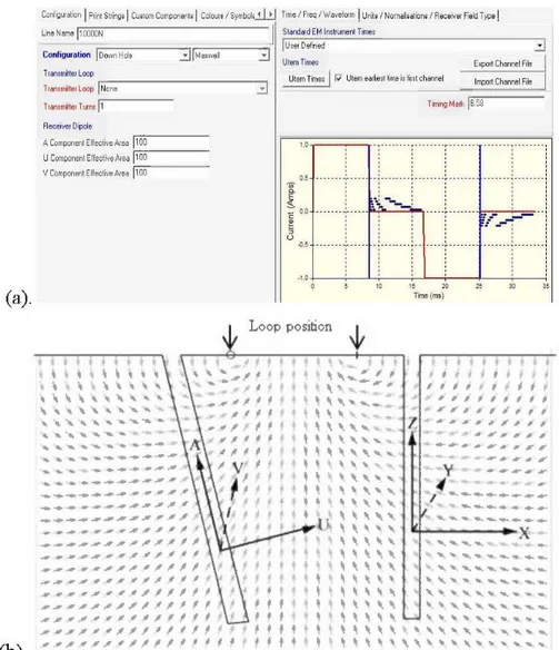
The w indow below (Figure 3.2(a)) shows how to set up the pararneter values of the measurement system. We considered a Geonic system (Protem 25Hz) w ith the component effective area of three components of 100, transmitting frequency is determined as 30Hz . The component effective area is calculated by: area of a single tum x nurnber of tums x amplification coefficient. A represents axial component:, i.e., along the drill hole, painting upward. U is a component transverse to axial and in the vertical plane containing the drill ho le, at 12 o' clock when looking clow n the hole. V also is a component transverse to axial and in the vertical plane containing the drill hole, at 12 o' clock when looking clown the hole. Components A, U and V are corresponding to Z , X and Y, respectively. See Figure 3.2(b).
CHAPTER III. Numerical simulation ofborehole electromagnetic signais
(a).
(b).
Configuration 1 Print StlingsJ Custom ComponentsJ Colours / Symboh~ Time 1 Freq 1 'Waveform 1 Units 1 Nornalisations 1 Receiver Field Type 1
Line Name j10000N
J
Standard EM Instrument Timesr::---;:-.,---,177- , . - - - - . . , - JuserDefined :::1
Configuration 1 Down HQI~ o::::JI Maxwell iJ Utem Times
Export Channel File -,
Tr<Y~s:mitter Loop
Tr011smittor LOOj) ~~N:-one---, :::1 Tr~s:mitter TLKns: p
Aeceiver Dipoie A Component EffecliveArea j100
U Componenl Effective Area "'J10:::;-0
-V Component EffectiveArea J100
Utem Times 1 P' Utem earliest tim;l is tirst channel lmport Ch<!!nnel File 1
h rrir!l Mork 18.58 1 0 . , ... , ... , ' ' ' ' ' ' 1 1 1 ' ' ' 1 ' ' ' 1 ' ' ' 1 ' ' ' 1 1 0.~ •.••••• ·:· ••••• "1"" ... ! ... --~ -... ~ -... j
J: :
~-=
; ;--;
J
-1.0 0,,
,,
"
Time (ms) " Loop position._ ... ----"""41'
_...,.____
.,.,,, -.--~_....,,,.,,___
_.._...,..,,,,.;~_
_.._,.,..,....,.,,,,.~,,~~ _ ... _. ... ,,,_,;tt,; ..,._,_,,,,,,~/~ _..,..,.,,.,,,,,_,,...
,,,,,,,_,,,
..,,,,,,,,_,_,_,, ~,,,,,,,,,,,""'''"'"""''''
"'"''"""""''''
.,.,,,,,
1111111 , , 1 1 1 1 1 1 ; 1 #'1'~ • • , , , ,.,,.,.,.~,, , . , , , , , , ; _..,.,.,.,,.,,..
,.~~"""'_
_..,...,..,,--
...
~ -..-...
..-~ 16j
Figure 3.2 (a) Parameter values setup window for measurement system; (b) Components sketch map and the corresponding relationship between A, U, V and X, Y, Z.
Figure 3.3 shows positions and size of the transmitter loop and the plate. For the space of the figure, we just give out three loops: centre, east and north. There are other two loops which situate on the west and south side, respectively.
CHAPTER III. Numerical simulation ofborehole electromagnetic signais 1 1 lv-~ 1 1 1
•
(b) top viewL
1 l east pL•te 1 \ 1 d0\\1lhole plate \ ~""'
,,
Figure 3.3 A sketch ofloop 's and plate's size and positions
17
The thin plate's parameters are set in the window below (Figure 3.4). Common values for each madel used in this research are: size of plate is 150mx 150m,
azimuth is 270°, conductivity of the plate is lOOS·m-1. The simulation results can
be visualized very quick:ly in the window at the right side.
Dioplay Oisp, Ch.!lns. 1%11.%~
1
1~m~
Oisp_ Ault Phn Field IOOOON
""'" Ch. Vect01 1 l.igh<rog
œa
,...
( Plates OsiiPiarmet Algorllhn 1 la.,.. Eatth << 1 Add 1 Delelej » j ~ Copy 1 Colms l -tOO lt 3 P Cale. r ..., co~e. ·200 r ThickPI. r R tT J":"P Use ln Auto Scate
Sroolate Overt::uden
jNo OB Sinulation :::::::J .,..
l.fuJIO<JII
jNone 3
C HAPTER III. Numerical simulation ofborehole electromagnetic signais 18
3.2 Three-dimensional numerical simulation
In order to look at the impact on BHTEM signal variations from different geological occurrences of the conductor, combining with the variations of measurement system's configuration, we determined a series of situations for 3-D modeling as stated in Table 3.1.
Table 3.1 Values of param eters involv ed in num erical simulation
Occurrence of the conductor Location Loop location of the conductor related to the drill-hole Horizontal In the East of the hole Centre
Dip 45 ° to west In the West of the hole East In the South of the
Vertical South
ho le
Dip 45° to west Penetrated by ho le West
Below the hole North
The first column contains the different dip angles of the thin plate that are typical occurrences in space. The second column indicates the location of the thin plate related to the drill-hole. The third column is the transmitter loop 's location related to the drill-hole. The simulation results are divided into five model series according to the location of the thin plate (the second column). Each model series is then divided into four sub-series, reflecting changes in the inclination of the conductor (first column). In addition, each subseries also contain five possible transmitter loop positions for the measurement system related to the conductor. Therefore, there are 5 x 4 x 5
=
100 models for a given drill-hole. We describe simulation results by series.3.2.1 Model Series 1
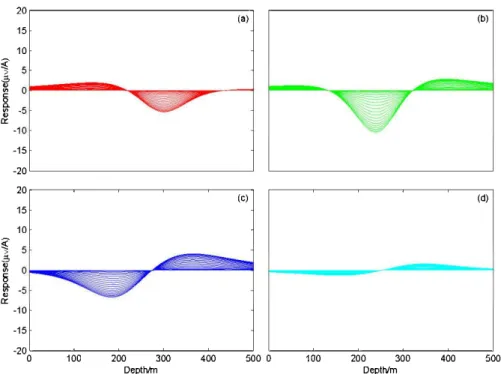
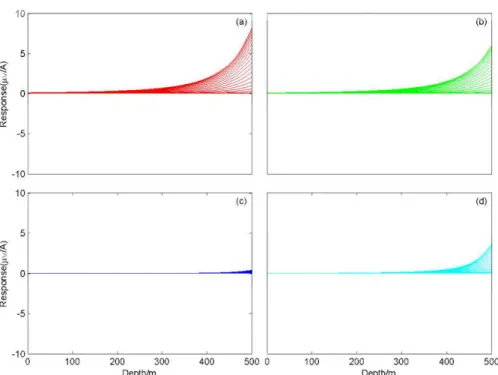
The plate situates on west side of the drill hole; the depth of its centre point is 300m. The distance from the centre point of the plate to the intersection point of drill hole and the horizontal plan which contains the centre point of the plate is 173m. See Figure 3. 5.
CHAPTER Ill Numerical simulation ofborehole electromagnetic signais ·100 ·200 ·300 -400 Il u
v
1 1 1Figure 3. 5 The mode! sketch of Mode! Series 1
19
The cornponent V in this rnodel series is zero; we only have cornponents A and U that are presented in following figures.
20 r---~ 15 10 -10 -15 -20 20 15 10
?
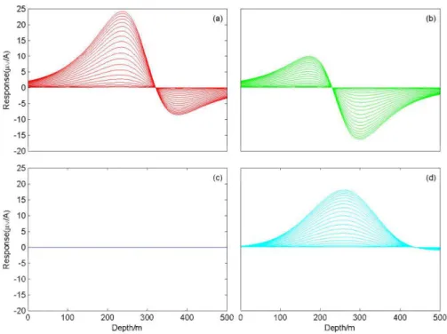
5 4 (8) (c) ~ or---~ §_ :6 -5 0:: -10 -15 -20 0 100 200 :>00 400 500 0 De pt hlm (b) (dJ 100 200 300 400 500 DeplhlmFigure 3. 6 The results of comp onent A of Mode! Series 1 wh en loop location is in the centre
C HAPTER III. Numerical simulation ofborehole electromagnetic signais 25 20 (a) (b) 15 ? 10 ], 5 "' "' !5 o. "' "' -5 Ir -1 0 -15 -20 25 20 (c) (d) 15 ? 10 ], 5 "' "' 8 0 o. "' "' -5 Ir -10 -1 5 -20 0 100 200 300 400 500 0 100 200 300 400 500 Depthlm Depthlm
Figure 3.7 The results of component U of Model Series 1 when loop location is in the centre (a) horizontal, (b) dip 45° to west, (c) vertical, (d) dip 45° to east
(a) 20 .---~ 15 10 ? 5 ],
~ 0~----~~--~~~~~
..
----~
8 ~ -5 Ir -10 -1 5 -20 L _ _ _ _ _ _ _ _ _ _ _ _ _ _ _ _ _ _ _ _ _ _ _ _ _ _ _ _ _ J 20.---~----~--~----~---. 15 10 ~ 5 ..:; ~ ol-. . ..,.'"' 8 ~ -5 Ir -10 -15 (c) -20 c _ _ _ _ _ . _ _ _ _ _ _ . _ _ _ _ ___. _ _ _ _ ___. _ _ _ _ _ _ J 0 100 200 300 400 500 0 Depthlm (b) -(d) 100 200 300 400 500 Depthlm 20Figure 3. 8 The results of component A ofModel Series 1 when loop location is in the east of drill ho le
CHAPTER III. Numerical simulation ofborehole electromagnetic signais 25 . - - - , 20 15 ? 10 > (a) ~ 5 ~
~ or---~~
~~~=~2~-~~~~._~
....
~
&! -5 -10 -15 -20L_ _ _ _ _ _ _ _ _ _ _ _ _ _ _ _ j 2 5 .---~--~-~--~---, 20 15 ? 10 ~ v 58
~ o ~o---__.. &! -5 -10 -1 5 (c) (b) (d) "20oc_---,-1 0~0--.,.-20~0--3~0-0--4~0-:-0--5::-'00 Oc_-~10~0--2::-'0-0--3~0-:-0--4~0-,-0 ---,-::-'500 Depthlm Depthlm 21Figure 3.9 The results of component U ofModel Series 1 when loop location is in the east of drill hole
(a) horizontal, (b) dip 45° to west, (c) vertical, (d) dip 45° to east
(a) 20 ,---~ 15 10 ? 5 _g ~ 0~--~~'-~~----~ g_ :tl -5 a:: -10 -1 5 -20L_---~ 20,---.,--~---.---.--~ (c) 15 10 ? 5 ~ ~ 0 ~---~ 8 ~ -5 a:: -10 -15 -20 L_-~L_-~--~--~--~ 0 1 00 200 300 400 500 0 De pt hlm 100 200 300 400 Depthlm (b) (d) 500
Figure 3.10 The results of component A ofModel Series 1 when loop location is the north of drill hole
C HAPTER III. Numerical simulation ofborehole electromagnetic signais 22 25 20 (a) (b) 15 ? 10 ], 5 ~ "' _....r-~ . _,;~ "' !5 0 o. "'
-"' -5 Ir -1 0 -15 -20 25 20 (c) (d) 15 ? 10 ], 5 "' "' 8 0 o. "' "' -5 Ir -10 -1 5 -20 0 100 200 300 400 500 0 100 200 300 400 500 Depthlm DepthlmFigure 3.11 The results of component U ofModel Series 1 when loop location is the north of drill hole
(a) horizontal, (b) dip 45° to west, (c) vertical, (d) dip 45° to east
(a) 20 ,---~ 15 10 ? 5 ], ~ 0~--~~'-~~----~ g_ :tl -5 Ir -10 -1 5 -20L_---~ 20,----.,----.---,---.----~ (c) 15 10 ? 5 ~ ~ 0 ~---~ 8 ~ -5 Ir -10 -15 -20 L_--~L_--~----~----~----~ 0 1 00 200 300 400 500 0 De pt hlm 100 200 300 400 Depthlm (b) (d) 500
Figure 3.12 The results of component A ofModel Series 1 when loop location is in the south of drill hole
C HAPTER III. Numerical simulation ofborehole electromagnetic signais 23 25 20 (a) (b) 15 ? 10 ], 5 ~ "' _....r-~ . _,;~ "' !5 0 o. "'
-"' -5 Ir -1 0 -15 -20 25 20 (c) (d) 15 ? 10 ], 5 "' "' 8 0 o. "' "' -5 Ir -10 -1 5 -20 0 100 200 300 400 500 0 100 200 300 400 500 Depthlm DepthlmFigure 3.13 The results of component U of Model Series 1 when loop location is in the south of drill hole
(a) horizontal, (b) dip 45° to west, (c) vertical, (d) dip 45° to east
(a) 20 ,---~ 15 10 ? 5 ], ~ 0~--~~'-~~----~ g_ :tl -5 Ir -10 -1 5 -20L_---~ 20,----.,----.---,---.----~ (c) 15 10 ? 5 ~ ~ or-,..E:;;;;; 8 ~ -5 Ir -10 -15 -20 L_--~L_--~----~----~----~ 0 1 00 200 300 400 500 0 De pt hlm 100 200 300 400 Depthlm (b) (d) 500
Figure 3 .14 The results of component A of Model Series 1 when loop location is in the west of drill hole
CHAPTER III. Numerical simulation ofborehole electromagnetic signais (a) 20 r---~ 15 10 ~ 5 ], ~ 0 ~--S§~ . . ~~~~~---~ §. ' ~~ :c-5 ~ Ir -10 -15 -20'--- - - - _ j 20r--~--r--~-~--~ (c) 15 10 ? 5 ], ~ O t--a~ 8 ~ -5 Ir -10 -15 (b) (d)
-20 o'---~1o~o--2o~o -~3o~o -~4o~o ---=-'5oo o·'---,-1 o~o----=-2o~o----=-3o~o--4o~o---=-'5oo
Depthlm Depthlm
24
Figure 3.15 The results of component U of Model Series 1 when loop location is in the west of drill hole
(a) horizontal, (b) dip 45° to west, (c) vertical, (d) dip 45° to east
A brief summary for numerical simulation results ofModel Series 1:
1. For the vertical plate, if we use east and west loop locations we can get obvious response and the response curves obtained by using these two transmitter loop locations are symmetric (see and compare Figure 3.8c, Figure 3.9c and Figure 3.14c, Figure 3.15c). For other loop locations the BHTEM signal of the plate is null (Figure 3.6c, Figure3.7c, and figures Figure 3.10c to Figure 3.13c).
2. For non-vertical plates (horizontal and inclined plates), we got the largest abnormal amplitude when the transmitter loop is centred over the hole (Figure 3.6 and Figure 3.7).
3. For the horizontal plate, we got same abnormal curves for east, north, south and west loop locations (figures Figure 3.8a to Figure 3.15a). And the centre loop location is the optimalloop location.
Thus for field measurements, we propose: when the target is vertical, the loop should locate on the east or west side of the hole. For other occasions the centred loop should be used.
0-!AP TER III. Numerical simulation ofborehole electromagnetic signais 25
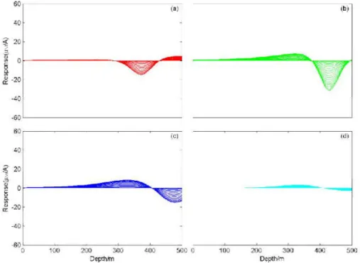
3.2.2 Model Series 2
The plate situates on east side of the drill hole; the depth of its centre point is
300m. The distance from the centre point of the plate to the intersection point of the drill hole and the horizontal plan which contains the centre point of the plate is
147m. See Figure 3.16. 10o400N 10300N 10200N 101(l0r.J 10000N OOOON OOOON 9700N
woou ~~~~~~~~~~~~~ ~~~~~=u~ 1~ooE
, . 1 , . 1 ~ :
:
~
· lOO .:zoo ·300 -400 .501)Figure 3.16 The mode! sketch ofModel Series 2
Values of component V in this model series are zero, so only components A and U are presented in following figures.
60 (a) (bj 40 ? 20 > -~ 01 ... = -!:j ~il-~ -20 ·40 -60l__ _ _ _ _ _ _ _ _ _ _ _ _ 60 ,--~----~--~-~iC-) (d) 40 -40
"60ol__ _ _ 1o'-:o---:2.,-,00--30-'-o,---~-'·oo.,---.,-,soo o 100 200 300 400 soo
Dep:Mn Oepthlm
Figure 3.17 The results of component A ofModel Series 2 when loop location is in the centre (a) horizontal, (b) dip 45 o to west, ( c) vertical, ( d) dip 45 o to east
CHAPTER III. Numerical simulation ofborehole electromagnetic signais 60 .---~(~a) 40 -40 -SOL---~ 60,---~.---~----~----~--~(~c) 40 -40 (b) (d)
-sooL_--~1o~o----2::-'o-=-o----3~o-=-o ----4~o_,-o ---==-'5oo o·c_--___,..,1 o~o----~2o~o----3~o-=-o----4~o-=-o----5::-'oo
Depthlm Depthlm
Figure 3.18 The results of component U ofModel Series 2 when loop location is in the centre (a) horizontal, (b) dip 45° to west, (c) vertical, (d) dip 45° to east
60 .---~(~a) 40 -40 -6Q L---~ 60 .---~.---~----~---~(~c) 40 ? 20 1 ~ 0 ~---~ 8 c. "' ~ -20 -40 -6Q L---~L---~----~----~----~ 0 1 00 200 300 400 500 0 De pt hlm 100 (b) (d) 200 300 400 500 Depthlm 26
Figure 3.19 The results of component A ofModel Series 2 when loop location is in the east of drill ho le
CHAPTER III. Numerical simulation ofborehole electromagnetic signais -40 -SOL---~ so.---~.---~----~----~--~(~c) 40 ? 20 J, ~ o r---~ 8 f,l-~ -20 -40 (b) (d)
-sooL_--~1o~o----2::-'o-=-o----3~o-=-o ----4~o-,-o ---==-'5oo o·c_--___,..,1 o~o----~2o~o----3~o-=-o----4~o-=-o----5::-'oo
Depthlm Depthlm
27
Figure 3.20 The results of component U ofModel Series 2 when loop location is in the east of drill ho le
(a) horizontal, (b) dip 45° to west, (c) vertical, (d) dip 45° to east
SO .---~(~a) 40 ? 20 J, ~
or---....
----~ g_ "' ~ -20 -40 -SOL_---~ so .---~.---~----~----~--~(~c) 40 ? 20 ~~ 0~---~~
8 c. "' ~ -20 -40 -SO L_--~L_--~----~----~----~ 0 1 00 200 300 400 500 0 De pt hlm 100 200 300 400 Depthlm (b) (d) 500Figure 3.21 The results of component A ofModel Series 2 when loop location is in the north of drill hole
CHAPTER III. Numerical simulation ofborehole electromagnetic signais 60 .---~(~a) 40 ? 20 ], ~ 0 ~---~----~ §_ "' ~ -20 -40 -SOL---~ 60,---~.---~----~----~--~(~c) 40 -40 (b) (d)
-sooL_--~1o~o----2::-'o-::-o----3~o.,.o ----4~o.,.o ---=-'5oo o·c_--...,.,1 o~o----~2o~o----3~o.,.o----4~o.,.o----5::-'oo
Depthlm Depthlm
28
Figure 3.22 The results of component U ofModel Series 2 when loop location is in the north of drill hole
(a) horizontal, (b) dip 45° to west, (c) vertical, (d) dip 45° to east
60 .---~(~a) 40 ? 20 ], ~
or---....
----~ §_ "' ~ -20 -40 -60L_---~ 60 .---~.---~----~----~--~(~c) 40 ? 20 ~~ 0~---~~
8 c. "' ~ -20 -40 -60 L_--~L_--~----~----~----~ 0 1 00 200 300 400 500 0 De pt hlm 100 200 300 400 Depthlm (b) (d) 500Figure 3.23 The results of component A ofModel Series 2 when loop location is in the south of drill hole
CHAPTER III. Numerical simulation ofborehole electromagnetic signais 60 .---~(~a) 40 ? 20 ], ~ 0 ~---~----~ §_ "' ~ -20 -40 -SOL---~ 60,---~.---~----~----~--~(~c) 40 -40 29 (b) (d)
-sooL_--~1o~o----2::-'o-::-o----3~o.,.o ----4~o.,.o ---=-'5oo o·c_--...,.,1 o~o----~2o~o----3~o.,.o----4~o.,.o----5::-'oo
Depthlm Depthlm
Figure 3.24 The results of component U ofModel Series 2 when loop location is in the south of drill hole
(a) horizontal, (b) dip 45° to west, (c) vertical, (d) dip 45° to east
60 .---~(~a) 40 ? 20 ], ~ 0 ~---~ §_ "' ~ -20 -40 -60L_---~ 60 .---~.---~----~----~--~(~c) 40 ? 20 ~ ~ 0~---~ 8 -c. "' ~ -20 -40 -6Q L_--~L_--~----~----~----~ 0 1 00 200 300 400 500 0 De pt hlm
-100 200 300 400 Depthlm (b) (d) 500Figure 3.25 The results of component A ofModel Series 2 when loop location is in the west of drill hole
CHAPTER III. Numerical simulation ofborehole electromagnetic signais 60 ~---~(a~) 40 ? 20 ], ~ o r---~ §_ "' ~ -20 -40 -60 L _ _ _ _ _ _ _ _ _ _ _ _ _ _ _ _ _ _ _ _ _ _ _ _ j 60,---~--~----~--~--~(c~) 40 ? 20 ],
~ 0~---~----~
f,l-~ -20 -40 (b) -(d)"60 o'---~1 o-,-o ---2~oo,---,3~oo----4o~o---=-'5oo o·'---~1 o-,-o ---2=-'"oo,---,3~oo,---4~oo---=-'5oo
Depthlm Depthlm
30
Figure 3.26 The results of component U ofModel Series 2 when loop location is in the west of drill hole
(a) horizontal, (b) dip 45° to west, (c) vertical, (d) dip 45° to east
A brief summary for numerical simulation results ofModel Series 2:
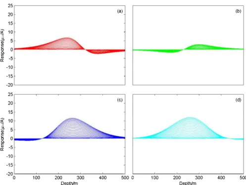
1. When the loop locates on east side of the hale, we can get largest amplitude of BHTEM signal, except for vertical plate of which amplitude is zero (Figure 3.19 and Figure 3.20).
2. The response curves obtained when the loop locates on south si de of the drill-hale are the same as those obtained when the loop locates on north side of the drill-hale (see and compare Figure 3.21, Figure 3.22 and Figure 3.23, Figure 3.24).
3. Abnormal signal is very weak when the loop locates on the west side of the hale, especially, for horizontal plate the abnormal signal is virtually zero (Figure 3.25 and Figure 3.26).
4. For vertical plate, the abnormal amplitude 1s largest when the loop 1s centred on the drill-hale (Figure 3.17c and Figure 3.18c).
Thus in field working for Madel Series 2 cases, following suggestions should be taken in consideration:
CHAPTER III. Nwnerical simulation ofborehole electromagnet ic signals 31
When the target is vertical, the loop should be centred over the hole. Other occasions the loop should be located on the east side of the hole in order to get strongest signal.
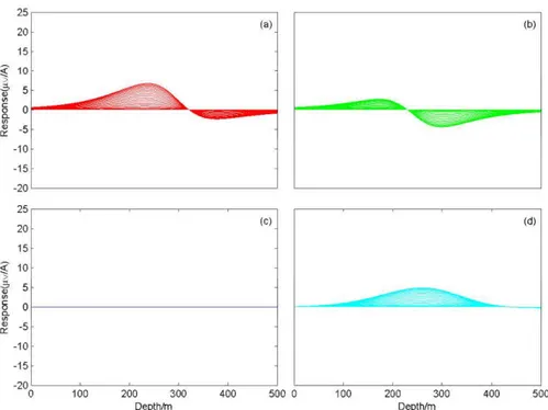
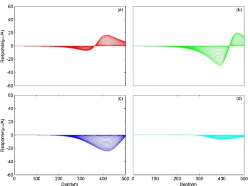
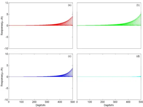
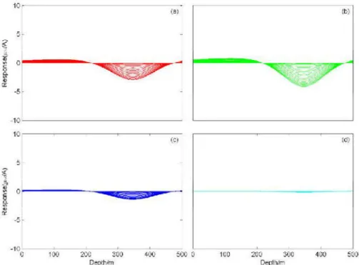
3.2.3 Model Series 3
The plate situates under the drill hole and the depth of its centre point through
which the extension line of the drill hole penetrates is 550m. See Figure 3.27.
~~~~~~~~10500E
1 1 1 1 1 1 1 1 1 1 1 1 1 1 1 1 ·100 ·200 ·300 ·400 ·000 -600 1 1 1 1 :v
Figure 3.2 7 The mo del sketch of Mo del Series 3
1\J:, Model Series 1 and 2, values of component V in this model series are zero, so only components A and U are presented in follmving figures.
CHAPTER III. Numerical simulation ofborehole electromagnetic signais 10 .---~ (a) 5 -5 -1QL---~ 10,---~.---~----~----~----~ (c) 5 -5 (b) (d)
--10 oL_--~1 o~o----2::-'o-=-o----3~o-=-o ----4~0-,-o ---::-'500 o·c__--___,..,1 o~o----~2o~o----3~o-=-o----4~o-=-o----5=-'oo
Depthlm Depthlm
Figure 3.28 The results of component A ofModel Series 3 when loop location is in the centre (a) horizontal, (b) dip 45° to west, (c) vertical, (d) dip 45° to east
10 .---~ (a) 5 ? .§, ~ o r---~ 8 c. V> " a:: ? .§, -5 -1Q L---~ 10.---~.---~----~----~---. (c) 5 ~ 0 ~---
..
~ 8 c. V> " a:: -5 - 1 Q L---~L---~----~----~----~ 0 1 00 200 300 400 500 0 De pt hlm (b) (d) 100 200 300 400 500 DepthlmFigure 3.29 The results of component U of Model Series 3 when loop location is in the centre (a) horizontal, (b) dip 45° to west, (c) vertical, (d) dip 45° to east
CHAPTER III. Numerical simulation ofborehole electromagnetic signais ? J, -5 - 1QL---~ 10 .---~~--~----~----~---, (c) 5 ~ 0 ~---1 8 f,l-"' a: -5 (b) (d)
-10 oL_--~1 o~o----2::-'o-=-o----3~o-=-o ----4~0-,-o ---::-'500 a·c__--___,..,1 o~o----~2o~o----3~o-=-o----4~o-=-o----5::-'oo
Depthlm Depthlm
33
Figure 3.30 The results of component A ofModel Series 3 when loop location is in the east of drill ho le
(a) horizontal, (b) dip 45° to west, (c) vertical, (d) dip 45° to east
? J, 10 . - - - -- , (a) 5 ~
or---. ..
.a
R
-"' "' a: ? ~ -5 - 10L_---~ 10.---~~--~----~----~---, (c) 5 ~ o r---~ 8 c. "' "' a: -5 -1Q L_--~L_--~----~----~----~ 0 1 00 200 300 400 500 0 De pt hlm 100 200 300 400 Depthlm (b) (d) 500Figure 3.31 The results of component U ofModel Series 3 when loop location is in the east of drill ho le
CHAPTER III. Numerical simulation ofborehole electromagnetic signais ? ], 10 r---~ (a) 5 ~ 0 ~---~~ §_ "' "' Ir ? ], -5 -1QL---~ 10r---~r---~----~----~----~ (c) 5 ~ 0 ~---~~ 8 f,l-"' Ir -5 (b) (d)
-10 oL_--~1 o~o----2::-'o-=-o----3~o-=-o ----4~0-,-o ---::-'500 o·c__--___,..,1 o~o----~2o~o----3~o-=-o----4~o-=-o----5=-'oo
Depthlm Depthlm
34
Figure 3.32 The results of component A ofModel Series 3 when loop location is in the north of drill hole
(a) horizontal, (b) dip 45° to west, (c) vertical, (d) dip 45° to east
? ], 10 r---~ (a) 5 ~ o r---~ §_ "' "' Ir -5 -10L_---~ 10r---~r---~----~----~----~ (c) 5 ? ~ ~ 0 ~---~~ 8 c. "' "' Ir -5 -1Q L_--~L_--~----~----~----~ 0 1 00 200 300 400 500 0 De pt hlm 100 200 300 400 Depthlm (b) (d) -500
Figure 3.33 The results of component U ofModel Series 3 when loop location is in the north of drill hole
CHAPTER III. Numerical simulation ofborehole electromagnetic signais ? ], 1 0 r---~ (a) 5 ~ 0 ~---~~ §_ "' "' Ir ? ], -5 - 1 QL---~ 1 0r---~r---~----~----~----~ (c) 5 ~ 0 ~---~~ 8 f,l-"' Ir -5 (b) (d)
-10 oL_--~1 o~o----2::-'o-=-o----3~o-=-o ----4~0-,-o ---::-'500 o·c__--___,..,1 o~o----~2o~o----3~o-=-o----4~o-=-o----5=-'oo
Depthlm Depthlm
35
Figure 3.34 The results of component A ofModel Series 3 when loop location is in the south of drill hole
(a) horizontal, (b) dip 45° to west, (c) vertical, (d) dip 45° to east
? ], 10 r---~ (a) 5 ~ o r---~ §_ "' "' Ir -5 - 1 0L_---~ 10r---~r---~----~----~----~ (c) 5 ? ~ ~ 0 ~---~~ 8 c. "' "' Ir -5 -1Q L_--~L_--~----~----~----~ 0 1 00 200 300 400 500 0 De pt hlm 100 200 300 400 Depthlm (b) (d) -500
Figure 3.35 The results of component U ofModel Series 3 when loop location is in the south of drill hole
CHAPTER III. Numerical simulation ofborehole electromagnetic signais ? ], 10 r---~ (a) 5 ~ o r---~ §_ "' "' Ir ? ], -5 -10 L__ ________________________ _ j 10r---~----~----~--~----~ (c) 5 ~ 0 ~---~~ 8 f,l-"' Ir -5 36 (b) (d)
--10 oL__---,1~oo,----2c:-'o-=-o ---=-3o~o----4~o.,--o ---::-'5oo o·L__---,1~oo,----~2o~o---=-3~oo,----4~o-=-o ---::-'5oo
Depthlm Depthlm
Figure 3.36 The results of component A ofModel Series 3 when loop location is in the west of drill hole
(a) horizontal, (b) dip 45° to west, (c) vertical, (d) dip 45° to east
? ], 10 r---~ (a) 5 ~ 0 ~---~ §_ "' "' Ir -5 -10 L _ _ _ _ _ _ _ _ _ _ _ _ _ _ _ _ _ _ _ _ _ _ _ _ _ _ __J 10r---~----~----~--~----~ (c) 5 ? ~ ~ 0 ~---~ 8 c. "' "' Ir -5 -10 L _ _ _ _ _ _ . _ _ _ _ _ _ . . _ _ _ _ _ . . _ _ _ _ _ . _ _ _ _ _ __J 0 1 00 200 300 400 500 0 De pt hlm 100 200 300 400 Depthlm (b) (d)
-500Figure 3.37 The results of component U ofModel Series 3 when loop location is in the west of drill hole
(a) hori zontal, (b) dip 45° to west, (c) vertical, (d) dip 45° to east
As we said before, nowadays, shallow deposits are rarer and rarer, and deep deposits will definitely become the main targets in the future. But methods