Can Gravitation Anisotropy Be Detected by
Pendu-lum Experiments?
René Verreault
Department of Fundamental Sciences, University of Quebec at Chicoutimi, 555, Boul. de l'Université,
Saguenay (Quebec), Canada G7H 2B1
[email protected]
Abstract. After some 170 years of Foucault pendulum experiments, the linear theory fails to quantitatively explain the results of any honest meticulous experiment. The pendulum motion usually degenerates into elliptical orbits after a few minutes. Moreover, unexplained discrepancies up to ±20% in precession velocity are not uncommon. They are mostly regarded as a con-sequence of the elliptic motion of the bob associated with suspension anisotropy or as a lack of care in starting the pendulum motion. Over some 130 years, an impressive amount of talented physicists, engineers and mathematicians have contributed to a better partial understanding of the pendulum behaviour. In this work, the concept of biresonance is introduced to represent the motion of the spherical pendulum. It is shown that biresonance can be represented graphically by the isomorphism of the Poin-caré sphere. This new representation of the pendulum motion greatly clarifies its natural response to various anisotropic situa-tions, including Airy precession. Anomalous observations in pendulum experiments by Allais are analyzed. These findings suggest that a pendulum placed within a moving mass distribution such as the earth, the moon and the sun near a syzygy should be treated as if a rotating gravitational field would produce a Coriolis-like acceleration and influence precession.
Keywords: Pendulum, gravitation, anisotropy, Poincaré sphere, biresonance, linear biresonance, circular biresonance, syzygy.
1. Introduction
After Galileo’s sentencing in 1633 for teaching, according to Copernicus’s view, that the earth was rotating under a sky with fixed stars, it took 218 years for someone to come up with the first experimental proof of the planet’s rotation. Jean Bernard Léon Foucault [1] had indeed noticed in 1851, while working on a lathe in his cel-lar, that the free end of a slender rod vibrating in a vertical plane retained its vibration direction unchanged even when the chuck was rotated by hand. Transposing that rod to a long vertical wire clamped in a fixation rigidly linked with the earth, he figured out that, from inertia, a swinging mass at the end of the vertical wire should be-have similarly with an eventually rotating earth.
As early as May 1851, G.B. Airy [2], Astronomer Royal, showed that, when the pendulum bob had elliptical trajectories, the nonlinear restoring gravitational force resulted in a tendency for the ellipse to undergo precessing motion. A major improvement occurred in 1879 with the doctor thesis of a certain Heike Kamerlingh Onnes [3], who incidentally ended up, a few decades later, with the discovery of superconductivity and was awarded a Nobel Prize. Throughout his 290 pages of equations, Kamerlingh Onnes demystified some of the unwanted elliptical or-bits of the pendulum as being caused by suspension anisotropy. Even today, a perfect isotropic suspension has not yet been achieved, though the principal consequences can be accounted for by calculation. Other significant con-tributions to the understanding of the Foucault pendulum have been made by Chessin (1895) [4], MacMillan (1915) [5], Longden (1919)[6], Noble (1952)[7], Somerville (1972)[8], Olsson (1978)[9], Latham (1980)[10], Hecht (1983)[11], Nelson et al. (1985)[12] and Pippard (1988) [13].
2 Verreault
Nevertheless, all those Foucault pendulums built since 1851 were meant neither to make precise measure-ments of the earth rotation velocity, nor to ride between the earth and the moon [14]. Their most frequent use was to serve as an utterly simple pedagogical instrument for illustrating some basic laws of physics or, in a similar way, to artistically decorate museums and institutes while promoting science for the general public. In those implemen-tations, the major drawback of the free (ordinary) pendulum was the rapid decay of its oscillations. In an article by Moppert et al. [15], it is stated, even some 130 years after Foucault’s original performance, that «with an ordinary pendulum, a run takes at the most, three hours…» It is then not surprising that physicists and engineers took the challenge of designing systems that would sustain the oscillations indefinitely.
Pioneering work in that sense was achieved by Fernand Charron [16], professor of physics at the Université catholique d’Angers, France. The pendulum swing was amplified by synchronized magnetic impulsions (paramet-ric amplification) until the wire would touch the inner part a f(paramet-riction ring (the Charron ring) placed a few centime-tres below the suspension point. Any lateral movement of the wire at the end of the swing was therefore efficiently damped, so that the tendency to generate ellipses was hindered. Practically all sustained pendulums used for public demonstration incorporate such damping rings, in order to retain nice rectilinear, large amplitude oscillations. But, all in all, it seems that the free pendulum still possesses one good quality that is inherent to many untamed, unsta-ble systems, namely some kind of hypersensitivity.
Speaking of untamed pendula, a word must be said about suspension systems. Every «textbook» pendulum is in fact a mathematical idealization where a point mass turns about a fixed suspension «point». Such a mathemati-cal pendulum consisting of a point mass moving on a spherimathemati-cal surface has two degrees of freedom. However real life pendula involve a spatially extended mass moving about a mobile instantaneous center of rotation located somewhere within the strained region of a clamped wire or inside the deformed contact area of a sharp (initially) point or knife edge. The heavily strained suspension region is subject to permanent deformations which alter an essential characteristic of a pendulum: its putative constant length. Moreover, the extended bob can spin about its wire (or rod) axis, which adds a third degree of freedom with an elastic restoring torque (clamped wire) or a dissi-pative friction torque (point contact).
In a tentative to minimize the above problems, the French engineer Maurice Allais designed the paraconical pendulum [17], which consists of a disk (the bob) connected by a rod to a vertical stirrup whose upper inner sur-face holds a steel ball rolling on an optically flat steel sursur-face. The suspension losses are significantly reduced. With that system, he made the unexpected discovery in 1954 of the so-called Allais effect. Allais used to design 30-day long experiments, day and night, restarting the pendulum every 20 minutes for 14-minute runs while allo-cating 6 minutes for the restart phase in the azimuth achieved at the end of the preceding run. In this way, he could detect the lunisolar periodicities of the tides in the time series of the azimuth changes at the end of the 14-minute runs. That phenomenon has not yet been explained up to now. Moreover, during one of those 30-day experiments in 1954, the pendulum showed a factor 5 change in precession speed as a total solar eclipse was passing some 1300 km away near Oslo [18]. Most scientists refer today to this «eclipse effect» as the Allais effect. It should be pointed out, though, that the eclipse effect and the above mentioned sensitivity to lunisolar tide periodicities should probably be considered as two distinct phenomena.
As Allais could repeat the observation of his eclipse effect in 1959, he started questioning the laws of gravita-tion according to Newton and Einstein. He was from then on denied credibility by the scientific establishment and he lost his financial support. That new Galileo recycled himself as an economist whose new theories earned him a Nobel Prize in 1988. After his death in 2010, a few dozen disciples [19, 20] from the physics, mathematics and
en-gineering communities are still chasing eclipse effects not only with paraconical and Foucault pendula, but with torsion balances [21, 22] and microgravimeters [23, 24].
In this paper, a new approach in describing the pendulum dynamics is presented. This sheds a new light on Allais’s experiments, clarifying the complex interaction between the Foucault effect and the anisotropic properties of the pendulum environment. This is especially useful for interpreting such nonlinear pendulum response as the Airy effect and its role in Allais’s findings. A new interpretation of some of Allais’s results follows.
2. Theory
2.1. Linear theory for harmonic oscillators
The theory is based on an isomorphism between the oscillation states of the pendulum and the points on the surface of a sphere. It turns out that this isomorphism is a dual theory of Poincaré’s mathematical theory of light, published in 1892 [25]. Poincaré studied the spatial changes of the vibrating electric field when light progresses through an anisotropic medium. An illustration of the use of the Poincaré sphere for describing the complex re-sponse of anisotropic crystals to magneto-optic excitation (induced circular birefringence) can be consulted in the author’s dissertation [26]. Here we study the temporal changes of the mechanical vibrations of a pendulum submit-ted to an anisotropic potential well [27].
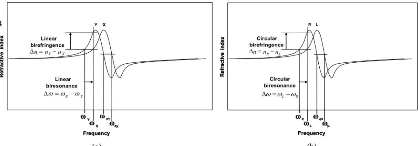
If one considers the dispersion curves of the refractive index about a resonant frequency of the atoms in an anisotropic crystal, there are two distinct absorption frequencies for light with two orthogonal rectilinear vibrating directions of the electric field. Classical electromagnetism considers then different resonant frequencies for the electron-nucleus system in matter, or for the system made of the electron gas versus the crystal lattice. Linear bire-fringence is the difference in refractive indices or the difference in velocity through matter for two orthogonal lin-early polarized light vibrations X and Y at the same frequency (Figure 1). Similarly, circular birefringence is the difference in refractive indices for two orthogonal circularly polarized light vibrations R and L at the same fre-quency.
Birefringence considers the polarization changes spatially along the path through the medium. Let us define linear biresonance as the difference in absorbing frequencies for two orthogonal linearly polarized light vibrations progressing at the same speed through matter (hence with the same refractive index). Let us define circular bireso-nance as the difference in absorbing frequencies for two right-handed and left-handed circularly polarized light vi-brations progressing at the same speed through matter (hence with the same refractive index)., Contrary to bire-fringence which is an environmental phenomenon at the wavelength scale, biresonance is a local phenomenon at the particle scale. It considers the local motion of the electron cloud centre of mass relative to a nucleus. That local motion ought to be rectilinear, circular or in general elliptical.
4 Verreault
(a) (b)
Figure 1. Definition of linear (a) and circular (b) biresonance as a difference in resonant frequencies at constant refractive index instead of a difference in refractive indices at constant frequency for birefringence.
The mechanical electron-nucleus system reacts as a harmonic oscillator. The idealized point mass Foucault pendulum is also a 2-D harmonic oscillator. Hence the general oscillation state of the pendulum can be represented by the same ellipses as does polarized light, as shown by Figure 2.
With reference to a rectilinear vibration along the X-axis, the ellipse is characterized by the azimuth ψ of the major axis and the ellipticity angle
tan1( / )
b a
, the minor to major axis ratio. Finally, the direction of travelalong the ellipse can be counter-clockwise (left handed orbit) or clockwise (right handed orbit), as seen from the pendulum suspension point.
Figure 2. Parameters of a general pendulum elliptical orbit as seen from the suspension point.
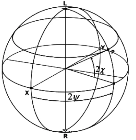
The isomorphism between the pendulum states and the geographic coordinates on the Poincaré sphere is shown in Figure 3. The equator represents the rectilinear vibrations in such a way that the longitude is twice the oscillation azimuth . Hence the orthogonal rectilinear states X and Y are diametrically opposed on the equator. The longitude of the point P representing an ellipse is twice the azimuth of the ellipse major axis. The latitude of the point P is twice the ellipticity angle. The northern hemisphere with positive ellipticities represents the left-handed elliptical pendulum orbits. The pole L is for the left-left-handed circular orbit. The southern hemisphere with
Y X Y X 0Y 0X R ef ra ct iv e in d e x Frequency Linear birefringence Linear biresonance X Y n n n Y X Y X Y X 0Y 0X R ef ra ct iv e in d e x Frequency Linear birefringence Linear biresonance X Y n n n Y X R L R L 0R 0L R ef ra ct iv ein d ex Frequency Circular birefringence Circular biresonance L R n n n R L R L R L 0R 0L R ef ra ct iv ein d ex Frequency Circular birefringence Circular biresonance L R n n n R L
Pendulum orbit parameters
b a X Y ) a b tan1 Ellipticity: Azimuth:
negative ellipticities represents the right-handed elliptical pendulum orbits. The pole R is for the right-handed cir-cular orbit.
Figure 3. The Poincaré sphere where P is the representative point of an elliptical orbit with azimuth
ψ
and ellipticity angleχ
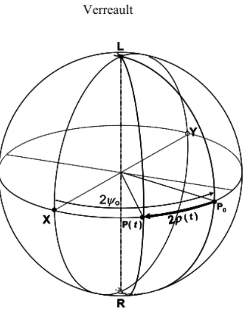
. Figure 4 shows the evolution of a pendulum with linear anisotropy. The orthogonal rectilinear eigenstates X and Y which remain unchanged with time determine an eigenaxis XY in the equatorial plane. The X state is taken as the fast axis (high frequency or long period of oscillation). A starting rectilinear state P0 with azimuth at 45 deg. from the X state will rotate at constant angular velocity about the XY axis as a function of time t. The counter-clockwise angle delta about the high frequency state X is equal to the phase shift after time t. One sees at the pole that after a 90 degree phase shift, the orbit was a left-handed circle.Figure 4. Evolution of the pendulum orbit represented by point P, with a start azimuth half way between the eigenaxes (45°), when pure linear biresonance is present. The phase angle grows linearly with time.
X Y L R 2 P 2 X Y L R X Y L R 2 P 2 2 P 2 P ( t ) 2o = 90° δ( t ) X Y L R P0 Gre atcirc le P ( t ) 2o = 90° δ( t ) δ( t ) X Y L R X Y L R P0 Gre atcirc le
6 Verreault
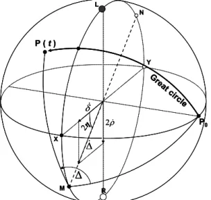
Figure 5. Evolution of the pendulum orbit represented by point P, with a rectilinear starting state P0, when pure circular bireso-nance is present. The phase angle is twice the precession angle:( ) 2 ( )t t . The rotation of P is counter-clockwise about the faster eigenstate R, which corresponds to the Foucault effect in the northern hemisphere.
Showing the case of circular biresonance as for the Foucault effect, Figure 5 pertains to a pendulum in the northern hemisphere of the earth. The orthogonal eigenstates of the pendulum which remain unchanged despite circular anisotropy are the two circular orbits of opposite sense. For an inertial observer airborne above the pendu-lum, the laboratory floor rotates counter-clockwise as well as the earth surface. Although the pendulum eigenstates are degenerate in the inertial reference frame, they have different angular velocities in the laboratory frame where the measurements of a Foucault experiment are made. As a matter of fact, due to the earth rotation, the right-handed circular orbit moves faster than the left-right-handed one in the laboratory frame. This causes a right-right-handed precession relative to the floor. On the Poincaré sphere, this is obtained through a rotation of the representative point P about the RL polar axis by a phase angle 2, the sense of the rotation being counter-clockwise about the fast state R.
Figure 6 shows the evolution of the pendulum orbit from a rectilinear starting state P0, when both linear and circular biresonance are present. The phase rates of change
and 2
measure the relative amount of each type of biresonance vectorially, the vectors pointing toward their respective fast states. The vector sum of linear and circu-lar biresonance defines the fast elliptic state M and the rotation axis MN for elliptic biresonance. The diametrically opposed states M and N are the elliptic orthogonal eigenstates with major axes at 90° from each other and with el-lipticities of opposite signs.X Y L R P0 2( t ) 2o P( t ) X Y L R X Y L R P0 2( t ) 2o P( t ) P0 2( t ) 2( t ) 2o P( t )
Figure 6. Evolution of the pendulum orbit represented by point P, with a rectilinear starting state P0, when both linear and cir-cular biresonance are present. The phase rates of change
and 2
measure the relative amount of each one. Linear and cir-cular biresonance add up quadratically to yield the amount of elliptic biresonance.2.2. Nonlinear Airy precession rate
The Airy effect is due to the anharmonicity of the restoring force, since actual pendula are not true harmonic oscillators. It is a form of induced circular biresonance which is proportional to the area of an elliptical orbit. It has the same sign as the ellipticity, so that the precession direction is the same as the rotation direction of the pendu-lum bob along the orbit. By itself, the Airy effect does not change the ellipticity. Hence, a perfectly isotropic pen-dulum started with an elliptical initial state would have the ellipse precess without changing its shape, and the rep-resentative point P on the Poincaré sphere would describe a small circle at constant latitude and constant velocity. The Airy precession rate is given by [9, 13]
2
3
8
A
ab l
,
(1)
where
pendulum swinging frequency; , ellipse semi-axes; pendulum length. a b l
Figure 7 illustrates the locus of the representative point P under the influence of Airy precession. The starting state 0 is a rectilinear vibration at an azimuth close to the slow axis Y. Since the pendulum already has a constant linear biresonance
, rotation of point P clockwise (cw) about the slow eigenstate Y brings it immediately into the northern hemisphere, which means the onset of a ccw elliptical orbit. The accompanying Airy precession rate at 2 R L M X N Y 2η
Δ
P0 P ( t ) Grea t circ le 2 R L M X N Y 2ηΔ
P0 P ( t ) Grea t circ le 2 R L M X N Y 2ηΔ
P0 P ( t ) Grea t circ le8 Verreault
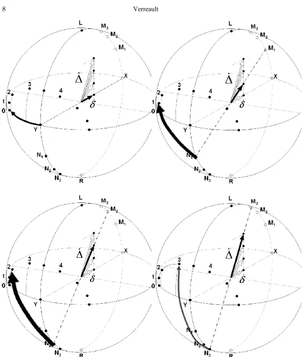
Figure 7. Evolution of the pendulum orbit as represented by the sequence 0, 1, 2, 3, 4…, with a rectilinear starting state 0 close to the slow eigenstate Y, when constant linear biresonance and induced Airy circular biresonance are present. The composite figure runs through 3 time increments. As soon as ellipticity sets in (time 1), Airy circular biresonance appears as a vertical component of phase rate of change, leading to a change in the rotation axis from XY to M1N1, and so on. The meridional points
Y, N1 , N2 , N3 show the sequences of the moving instantaneous centers of rotation of the radius vector describing the phase an-gle. The phase angle rate of change increases up to a maximum at time 3.5, as the module of the ellipse phase rate vec-tor(blackened) becomes maximal. The Airy contribution of circular biresonance is the polar component of, which equals
timestamp 1 changes the rotation axis from XY to M1N1. At the same time, the rotation rate (rate of phase change) increases since the module of
increases, while on the locus of P, the representative point also accelerates due to the longer radius about the instantaneous rotation axis M1N1 . The rapidly moving rotation axis MN away from thelocus of P causes the ellipticity to saturate (here at timestamp 3.5) when P crosses the meridian of the characteristic biresonance eigenplane XLYR. Airy precession, which is measured as twice the azimuth of point P, always accel-erates (or decelaccel-erates) toward the eigenplane and the slow state Y.
It is interesting to note that, for a harmonic oscillator (no Airy effect) with linear biresonance but in absence of Foucault effect (at the earth equator), the locus of P would be a small circle described at constant angular veloci-ty on the Poincaré sphere. The precession angle would oscillate about the eigenstate Y with an approximate sinus-oidal speed between two extreme azimuths: the rectilinear state 0 and its symmetrical rectilinear state on the oppo-site side of Y. However, to the first order of this theory of the anharmonic oscillator, the locus of P is no longer a circle but an oval with its long axis along the equator of the Poincaré sphere. On that oval, P accelerates from state 0, rushes through the eigenplane in the vicinity of state Y, decelerates to an about turn at the state symmetrical of 0 and then completes the cycle in the southern hemisphere with ellipses described in the opposite sense.
2.3 Mixture of linear biresonance, Airy effect and Foucault effect
The situation of Figure 8 represents a good quality anisotropic paraconical pendulum in the course of a 14 minute run. The polar vector accounts for a typical mid-northern latitudes Foucault precession rate
5
5 10
rad/s. The residual linear biresonance
amounts to ~30% of the “cosmological” circular contribu-tion 2. The slow elliptical eigenstate N0 lies then way up near the L pole. N0 will act as the first instantaneous rotation center for the radius vector joining the initial rectilinear state 0 and thereafter rotating cw about the N’s. At the start, the locus of P will progress perpendicularly to the radius vector N0-0 toward point 2 at essentially twice the Foucault precession rate, while N0 slowly switches to N2 during the first 2 minutes. The mobile state N accel-erates downward along the meridian of the eigenplane. After 7 minutes, the Airy precession rate completely com-pensates the Foucault rate, so that the mobile rotation axis MN coincides with the linear biresonance axis XY. Point 7 marks the end of precession in the Foucault direction. The rapid passage of state N through the equator of the Poincaré sphere is responsible for the abrupt kink in the locus of P at point 7, after which the Airy precession rate supersedes the Foucault rate. The subsequent deceleration of N, as state
N14 is approached, causes aquasi-rectilinear segment of the locus of P at point 14 and ellipticity saturation is reached (see the lower curves of Figure 9).
It can be seen in Figure 8 that after 14 minutes, the overall precession angle is back to nearly zero. In fact, there exists a critical starting azimuth con the Foucault direction side of the eigenplane azimuth Y where the 14-minute compensation is exact.
If the start state 0 lies within the interval [c
,
Y
], the initial segment of the locus is more parallel to the equa-tor and the ellipticity grows less rapidly. The Airy precession also grows more slowly and it does not quite com-pensate the Foucault precession after 14 minutes. There remains a net precession angle towardc.If the start state 0 outside the interval lies beyond state c, the initial segment of the locus makes a steeper angle with the equator, pointing into the northern hemisphere. The faster ccw ellipticity growth generates an over-compensating Airy precession which brings the final 14-minute azimuth closer to state c.
10 Verreault
If the start state 0 outside the interval lies beyond state Y, the initial segment of the locus gains readily the southern hemisphere into the domain of the cw ellipses. Airy precession and Foucault precession both act in the same direction and tend to bring the pendulum azimuth toward the interval [c
,
Y
].It is then clear that one can take advantage of that stabilizing property to experimentally determine the posi-tion of any unknown eigenplane and the direcposi-tion of the linear biresonance vector
. One only has to do chained experiments, where the start azimuth of run (i 1) is the final azimuth of run i. No matter the first start azimuth, the sequence of 14-minute azimuths converges to the critical state c, where the offset (c
Y
) is essentiallyde-termined by the amount of local Foucault effect and by the geometry of the ellipsoid of inertia. At the earth equa-tor, that procedure leads directly to the determination of the eigenstate Y.
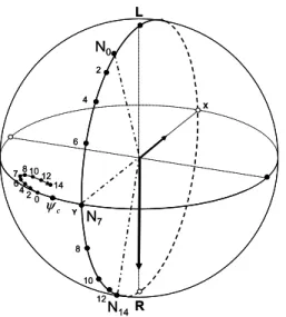
Figure 8. Locus of point P represented by the sequence 0, 2, 4, … 12, 14, with a rectilinear starting state 0 close to the slow ei-genstate Y, when constant linear biresonance, Foucault circular biresonance and induced Airy circular biresonance are present. A typical 14-minute run is considered. For the sake of clarity, the radius vectors linking the individual Ni to their corresponding point i on the locus of P are not shown. As soon as ellipticity sets in, Airy circular biresonance diminishes, nullifies and later overrides the Foucault circular biresonance vector shown. If the initial state 0 coincides with the critical azimuthc, then the final 14-minute azimuth comes back to the azimuthc .
3. A new interpretation of Allais’s pendulum experiments
As mentioned in the introduction, Allais performed chained experiments with his paraconical short pendu-lum. The instrument involved with Figures 9 and 10, due to suspension anisotropy, has a characteristic linear bi-resonance in the range 10% - 20% of the natural Foucault circular bibi-resonance in Paris. The data of Figure 9 origi-nate from a 15-day calibration experiment with a spherical bob [28]. From the orientation of the suspension beams, the estimated low frequency state Y should lie in the geographical azimuth of 206 °, measured cw from north. All the chained experiments are started at an azimuth 45° lower, namely 161°. Due to the Foucault effect and the Airy
R N14 Y X L 8 4 10 6 12 N0 N7 2 14 0 7 6 2 4 8 1012 c R N14 Y X L 8 4 10 6 12 N0 N7 2 14 0 7 6 2 4 8 1012 c
effect working in the same sense on that side of the low frequency state Y, it takes generally 5 to 7 runs for the 14-minute azimuths to cross over state Y and oscillate about a mean azimuth of 212.3°, which can be regarded as the critical azimuthc. Beside the Foucault effect influence, the offset of 6.3° cw can also be visualized as connected to the depth of the saddle shaped gravitational potential surface created by the suspension geometry.
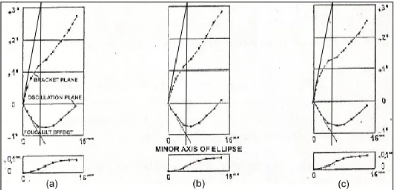
In Figure 9, let us concentrate our attention on the precession (middle) curves. From typical chained experi-ments reported on p. 104 and p. 140 of Ref. [28], the standard error on each point, as the mean value from 540 individual measurements in columns (b) and (c), is of the order of 0,01 grad. Hence the values of +0.07 grad and -0.15 grad for the respective 14-minute azimuths in the morning hours and in the evening hours are highly signifi-cant. They are correlated with the relative position of the moon with respect with the position of the pendulum in that 15 day period.
Figure 9. Full day (a) and half day (b and c) averages of spin angle (upper curve), precession angle (middle curve) and minor axis values (lower curve) after 14 minutes for Allais’s 15-day experiment Series VII, Sept. 21-Oct. 5, 1955. The angle units are grads. Columns (b) and (c) show the averages for the interval 0-12 h and the interval 12-24 h respectively. The Foucault rate is
5
2.94 grad/(14 min) 2.64 / (14 min) 5,5 10 rad/s
[29]. Note that the precession angle change becomes positive after 14
minutes during the morning hours (b), while it stays negative in the evening hours (c). Adapted from Allais' memoir to the NASA [30].
Figure 10. Averaged 14-minute run azimuths as a function of the approximate lunar time (25 solar hours per lunar day instead of 24h 50min) for the 30 day experiment from June 7 to July 7, 1955. The angle units are grads. The abscissa is labeled in mean solar time. Each point is an average over 28 lunar days. The 7.0 grad (6.3°) amplitude is very significant. (Graph reproduced from Ref. [28], p. 100).
12 Verreault
Figure 10 shows a detailed variation of the 14-minute azimuth for a particularly significant experiment in June-July 1955. Allais’s spectral analysis with a 24 solar hour cycle over 30 days yields an amplitude of 5.8 grad, while the adjustment over 28 lunar days gives 7.0 grad.
In general, all Allais’s one-month experiments showed a lunar cycle with amplitudes of the order of 1° in az-imuth, except those of fall 1954 and summer 1955 (Figure 10) with respective amplitudes of 5.8° and 6.3°. In 1954, that was in the month preceding an eclipse. In the middle of the summer 1955 experiment, on June 20, there was an eclipse through Thailand and the Philippines where the sun-moon-earth syzygy was particularly good. Since it is now established from the above theory that the final 14-minute azimuth, except for a given offset, con-verges toward the low frequency eigenstate determined by environmental anisotropy of the pendulum, the varia-tion of the 14-minute azimuth with a daily cycle suggests that the target eigenstate does undergo that daily cycle in azimuth with an amplitude of a few degrees.
The anisotropic pendulum behaviour can be interpreted in terms of shallow saddle potential superimposed over the spherical gravitational potential well. The low frequency eigenstate (longest swinging period) is in the az-imuth of the line of local potential minima. An isolated mass in the pendulum environment does not show revolu-tion symmetry about the pendulum axis. It will generate a saddle gravitarevolu-tional potential for the pendulum, where the line of local minima points toward that mass. In this way, the saddle potential due to the moon rotates under the pendulum according to the lunar day cycle. In order to be able to perturb the suspension anisotropy saddle by a few degrees daily, the lunar saddle must have a depth comparable with that of the suspension anisotropy saddle. However, independent calculations of the saddle potential from the moon by Allais [31] and by the present author fall short by ~7-8 orders of magnitude of the depth values for the suspension anisotropy saddle. Hence, the moon saddle potential cannot be held responsible for the observed oscillations of the anisotropy eigenstates Y. Those ob-servations call for some unknown property of gravitation.
4. Conclusion
In fact, pendulum motion is more complex than what can be explained by summing many two-body prob-lems: pendulum-earth, pendulum-moon, etc. In particular, the pendulum simultaneously lies in the far field of some distant masses and in the near field of an important mass distribution. As such, it should qualify for being addressed as an interior problem. Taking example with solid state physics and particle dynamics in solids, the con-cept of tensor effective mass has been successfully applied within Lorentz-Poincaré symmetry in crystals. It looks as if a tensor gravitational mass is needed, capable of describing accelerations not only along the classical line of action but also related to sideways motion. In kinematics, the Coriolis acceleration is successfully applied to the pendulum motion normal to a rotation axis. The equivalent link in dynamics appears to be missing, namely to rep-resent a rotating gravitational potential during a momentaneous syzygy.
References
[1] Foucault L. Démonstration physique du mouvement de rotation de la terre au moyen du pendule. Comptes rendus
hebdo-madaires des séances de l’académie des sciences, Vol. 32, p. 135-138, 3 février (1851).
[2] Airy G.B. On the Vibration of a Free Pendulum in an Oval differing little from a Straight Line. Proc. Royal Astron. Soc.,
Vol. XX, p. 121-130, May 9, (1851).
[3] Kamerlingh Onnes H. Nieuwe Bewijzen voor de Aswenteling der Aarde, Thesis, Rijksuniversiteit te Groningen, Gronin-gen, NL, 290 p., 1879
[4] Chessin A.S. On Foucault’s Pendulum. Am. J. Math., Vol 17, p. 81-88, (1895). [5] MacMillan W.D. On Foucault’s Pendulum. Am. J. Math., Vol 37, p. 95-106, (1915).
[6] Longden A.C. On the irregularities of motion of the Foucault pendulum. Phys. Rev., Vol. XIII, P. 251-258, (1919). [7] Noble W.J. A Direct Treatment of the Foucault Pendulum. Am. J. Phys., Vol. 20, p. 334-336, (1952).
[8] Somerville W.B. s. The Description of Foucault’s Pendulum. Q.J. Royal Astron. Soc., Vol. 13, 40-62, (1972). [9] Olsson M.G. The precessing spherical pendulum. Am. J. Phys., Vol. 46, p. 1118-1119, (1978).
[10] Latham R. An Interim report on a repeat of the Allais Experiment – the measurement of the rate of increase of the minor axis of a Foucault pendulum using automatic apparatus. I.C. Report G28, Imperial College, London, January 1980, 70 p. Available PDF at:
http://home.t01.itscom.net/allais/blackprior/latham/latham-rep28-1.pdf . Consulted May 18, 2010.
[11] Hecht K.T. The Crane Foucault pendulum : An exercise in action-angle variable perturbation theory. Am. J. Phys., Vol. 51, p. 110-114, (1983).
[12] Nelson R.A. and Olsson M.G. The pendulum – Rich physics from a simple system. Am. J. Phys., Vol. 54, p. 112-121, (1986).
[13] Pippard A.B. The parametrically maintained Foucault pendulum and its perturbations. Proc. R. Soc. Lond., Vol. A420, 81-91, (1988).
[14] For a Foucault pendulum in an Airbus, see:
http://www.youtube.com/watch?v=ToUCXRnlfog&feature=related. Consulted May 20, 2010.
[15] Moppert C.F. and Bonwick W.J. The new Foucault pendulum at Monash University. Q.J. R. Astron. Soc., Vol. 21, 108-118, (1980).
[16] Charron F. Bulletin de la SAF, Novembre 1931.
[17] Allais M. Observation des mouvements du pendule paraconique. CRAS, Tome 245, p 1697-1700, (1957).
[18] Allais M. Mouvement du pendule paraconique et éclipse totale de soleil du 30 juin 1954. CRAS, Tome 245, p 2001-2003, (1957).
[19] Duif C.P. A review of conventional explanations of anomalous observations during solar eclipses. arXiv:gr-qc/0408023 v5, 31 Dec. 2004.
[20] Munera H.A., ed. Should the laws of gravitation be reconsidered? :The scientific legacy of Maurice Allais. Apeiron, Mon-treal, Canada. 447 p., 2011.
[21] Saxl E.J. and Allen M. 1970 Solar Eclipse as «Seen» by a Torsion Pendulum. Phys. Rev D, Vol.3, p. 823,( 1971). [22] Kuusela T. Effect of the solar eclipse on the period of a torsion pendulum. Phys. Rev. D 43, p. 2041, (1991).
[23] Duval M. An Experimental Gravimetric Result for the Revival of Corpuscular Theory. Phys. Essays 18, 53-62, (2005). Results first presented at 69e Congrès de l’ACFAS, Sherbrooke, Qc., Canada, 13-17 May 1996.
[24] Duval M., Vérification expérimentale de la théorie corpusculaire de la gravitation. http://arxiv.org/ftp/arxiv/papers/0705/0705.2581.pdf (2007).
[25] Poincaré H. Théorie mathématique de la lumière, Vol. II, Ch. 12., Gauthier-Villars, Paris, 1992.
[26] Verreault R. A new method to measure general birefringence in crystals. Zeitschrift für Kristallographie 136, 350-386 (1972).
[27] Verreault R. Can Santilli Gravitational Anisotropy Be Detected Via Pendulum Experiments? San Marino Workshop on Astrophysics and Cosmology for Matter and Antimatter. San Marino, Italy, September 5-9, 2011. Lecture 10 on http://www.world-lecture-series.org/san-marino-2011,
[28] Allais M., L'Anisotropie de l'Espace Clément Juglar, Paris (1997), p. 81-101. [29] Allais M., L'Anisotropie de l'Espace Clément Juglar, Paris (1997), p. 93.
[30] Allais M., The "Allais Effect" and my Experiments with the Paraconical Pendulum 1954-1960, a memoir prepared for NASA, 1999, available online at: http://www.allais.info/alltrans/nasarep.htm.