Modelling of split hopkinson pressure bars : adaptation of a compression apparatus into tension

(1)

HUGUES BERGER-PELLETIER

MODELLING OF SPLIT HOPKINSON PRESSURE

BARS

Adaptation of a compression apparatus into tension

Mémoire présenté

à la Faculté des études supérieures et postdoctorales de l’Université Laval dans le cadre du programme de maîtrise en Génie Mécanique

pour l’obtention du grade de Maître ès sciences (M.Sc.)

DÉPARTEMENT DE GÉNIE MÉCANIQUE FACULTÉ DES SCIENCES ET DE GÉNIE

UNIVERSTÉ LAVAL QUÉBEC

2013

(2)

II

Résumé

Les Barres d’Hopkinson sont couramment utilisées pour tester les matériaux à des hauts taux de déformations. Souvent, différents systèmes de barres sont utilisés pour tester les matériaux en tension ou en compression.

Par contre, il serait pratique d’utiliser un seul système, pour prendre des mesures en tension et en compression. Des études ont été faites pour convertir le système de compression existant du centre de Recherche et Développement pour la Défense Canada (RDDC) de ValCartier.

Un concept a été choisi parmi 6 systèmes de tension déjà existants. Le choix a été validé avec un modèle d’éléments finis fait sur LS-Dyna. Le modèle a été calibré sur des résultats de compression fournis par le RDDC. Il fut ensuite modifié pour intégrer le nouveau concept.

À cause d’un manque de ressources, les résultats de simulation sur LS-Dyna n’ont pu être comparés avec des résultats expérimentaux, puisqu’un premier prototype n’a pu être fabriqué.

(3)

III

Abstract

The Split Hopkinson Pressure Bars (SHPB) is a common method used to characterize materials at high rates of strain. First used to experiment on materials in compression, the method was adapted to do tests in tension and torsion. The compression apparatus consists of a specimen sandwiched between 2 pressure bars, called the input bar and the output bar. A third bar, the striker, is launched at the input bar. Upon impact, a compressive pulse traveling toward the specimen is generated. This load is partially transmitted into the specimen and the output bar, the rest of it being reflected back into the input bar. Using measurements of the input, transmitted and reflected pulse, it is possible to develop the stress-strain response of the material deforming at high strain rates. This is achieved using strain gages adequately placed on both pressure bars.

Many researchers use a different SHPB system when it comes to tension tests. Many methods exist, but all of them are based on compressive experiments. It would therefore be convenient to only have one system, which is capable of taking measurements both in compression and tension. Based on the compressive SHPB apparatus used by the Defense, Research and Development Canada (DRDC) center in ValCartier, studies were made to convert the compressive system into a tensile setup.

The goal was to modify it with minimum changes possible, in order to easily go back and forth between the two configurations. A design choice was made, considering 6 existing tension systems. To validate the decision, a finite element model was created using LS-Dyna. The modal was first aligned with the compression results provided and then modified to implement the selected design. Because of a lack of available resources, LS-Dyna simulation results were not compared with experimental data, as it was not possible to create a first prototype.

(4)

IV

Acknowledgements

This research project would not have been possible without the support of many people. I wish to express my gratitude to Professor Augustin Gakwaya, who offered great help and whose assistance was always crucial.

I also wish to express my sincere thanks to Réjean Arsenault, who was a mentor through this project.

Moreover, I am deeply appreciative of Manon Bolduc’s support and supervision; that made it possible to complete this research.

Special thanks to Dennis Nandlall that allowed me to work with a team of highly qualified professionals.

(5)

V

List of tables

Table 1: Methods advantages and disadvantages ... 16

Table 2: Scores for each advantages and disadvantages ... 18

Table 3: Tension methods total scores ... 19

Table 4: Aluminum and Steel properties ... 47

Table 5: Main dimensions of the SHPB setup ... 48

Table 6 : Comparison between theoretical and simulated stress values ... 52

Table 7 : Summary of the model properties and characteristics ... 58

Table 8: Johnson-Cook parameters for aluminum 6061-T6 ... 59

(10)

X

List of figures

Figure 1: Simple sketch representing a standard SHPB system ... 3

Figure 2: Example of stress versus strain curve obtained via SHPB testing [1] ... 4

Figure 3: Shu et al. tensile SHPB ... 10

Figure 4: Lee et al. collar/specimen assembly ... 11

Figure 5: Haugou et al. sleeve and specimen assembly ... 12

Figure 6: Haugou et al. full fixture ... 12

Figure 7: Fixtures after tensile loading. ... 13

Figure 8: Side bars apparatus ... 13

Figure 9 : Specimen used by Eskandari and Nemes ... 14

Figure 10 : Fixture and specimen assembly ... 14

Figure 11 : Hat specimen apparatus ... 14

Figure 12: Harding et al. assembly ... 15

Figure 13: Pressure wave traveling in a medium ... 24

Figure 14: Wave propagation from one bar to another ... 26

Figure 15: Typical specimen geometry... 28

Figure 16: General pulse shape ... 31

Figure 17: Wave front traveling through a bar, shown in a Lagrange diagram ... 31

Figure 18: Collar type of tension SHPB ... 32

Figure 19: Lagrange diagrams for tension and compression SHPB ... 33

Figure 20: Symmetry of a Lagrange diagram ... 33

Figure 21: Lagrange diagram showing the spurious wave ... 34

Figure 22: Lagrange diagram for a non-symmetrical SHPB apparatus ... 36

Figure 23 : Full Lagrange diagram for the proposed setup ... 39

Figure 24 : Typical SHPB setup ... 42

Figure 25: Nodes correspondence at bars extremities ... 42

Figure 26: Linear kinematic hardening representation ... 44

Figure 27 : Finer mesh at the end of the bars ... 48

Figure 28 : Typical mesh of the cross section ... 49

Figure 29 : The full model of the compression apparatus ... 50

(11)

XI

Figure 31 : Pulse going through the input bar for a striker speed of 17.3 m/s ... 51

Figure 32 : Results, at different striker speeds, presented in A. Bouamoul's report [19] . 52 Figure 33 : Results of the 3D model created for this thesis ... 53

Figure 34 : Standard specimen taken from ASTM volume 3.01 section E8M [22] ... 55

Figure 35 : Standard specimen shapes, with threaded ends, taken from ASTM volume 3.01 section E8M [22]... 56

Figure 36: Gap between the collar and the specimen ... 56

Figure 37 : Representation of the specimen with short ends and no threads ... 57

Figure 38 : Strains measured at the input bar strain gauges for each speeds ... 60

Figure 39: Strains measured at the output bar strain gauge, for each speed ... 61

Figure 40: Rise time for a 175 mm long striker ... 62

Figure 41 : Rise time for a 125 mm long striker ... 63

Figure 42 : Specimen stresses ... 64

Figure 43 : Input bar stress when only the collar is installed... 65

Figure 44: Stress in the output bar when only the collar is installed ... 66

Figure 45: Stress in the input bar when only the specimen is installed ... 67

Figure 46: Stress probed in the output bar ... 69

(12)

1

Chapter 1:

(13)

2

1.1 Uses of SHPB

Engineers, material specialists and scientists often use material properties in their calculations. For structural resistance, the elastic modulus, yield strength, ultimate strength, Poisson coefficient, etc. are important parameters required to determine any structure strength.

It is possible to find these parameters in handbooks and scientific papers, where their values are often based on experimental characterization methods. The most common experimental method used is the classical traction test, which gives a lot of information on a material, including the elastic modulus.

However, this test is performed at very low strain rates (in the order of 0.025 mm-s/mm [1]) and the material is therefore deformed very slowly. Most of the time, material behavior is different at higher strain rates of deformation. Consequently, when a design must take into account high rates of strain, it is preferable to use relevant material data. For example, a car crash simulation should be done using material properties at high strain rates. This data can be found experimentally using the Split Hopkinson Pressure Bars or SHPB, which is probably the most common way of finding material properties at high strain rates, including the widely used strains versus stress curve.

1.2 SHPB fundamentals

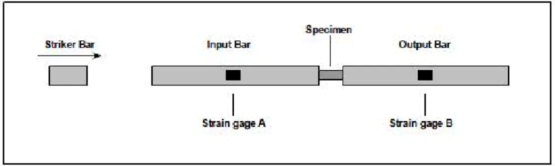
The standard SHPB (compression) setup includes 3 bars: the striker, the input bar and the output bar. Normally, these 3 bars are made of the same material. The striker is launched at the input bar at a specific speed. Upon impact, a stress pulse traveling toward the specimen is generated in the input bar. That pulse is then partially transmitted into the specimen and the output bar. The rest is reflected back into the input bar.

(14)

3 Figure 1 is a simple sketch representing a standard compressive SHPB system. The figure also shows 2 strain gages, one on each pressure bar. These gauges record the strains during the test. The duration depends mostly on the pressure bars materials and lengths.

Figure 1: Simple sketch representing a standard SHPB system

Often, the three bars are made of steel, with high yield strength. It is important that only the specimen deforms beyond its elastic limit. The following equations, calculating the specimen behavior in terms of the pressure bars strain history, are valid only if both bars are deformed within their elastic limit.

Based on wave propagation in solids, the stress in the specimen is given by [2]:

𝝈𝒔(𝒕) = 𝑬𝑨_{𝑨 𝜺}𝟎 𝑻(𝒕) (1.1)

Where 𝜎𝑠(𝑡) is the stress in the specimen as a function of time, 𝐸 and 𝐴0 are the pressure

bars elastic modulus and section respectively, 𝐴 is the specimen section and 𝜀𝑇(𝑡) is the

transmitted strain history (measured in the output bar).

The specimen strain history is found using the reflected pulse, measured in the input bar: 𝒅𝜺𝒔(𝒕)

𝒅𝒕 = − 𝟐𝑪𝟎

(15)

4 With this equation, the specimen strain rate 𝑑𝜀𝑠(𝑡)

𝑑𝑡 is found, using the input bar length 𝐿,

the wave speed of the wave in the bar 𝐶0 = �𝐸_𝜌 and the reflected pulse 𝜀𝑅(𝑡).

The strain is then calculated by integrating the previous equation:

𝜺𝒔(𝒕) = −𝟐𝑪_{𝑳 � 𝜺}𝟎 𝑹(𝒕)𝒅𝒕 𝒕

𝟎 (1.3)

Figures of stress or strain versus time are usually not relevant in engineering. Both curves are often merged together, in order to obtain the commonly used “Stress versus Strain” curve. An example of such a curve is presented in figure 2.

Figure 2: Example of stress versus strain curve obtained via SHPB testing [1]

The main problem encountered with SHPB is called the “spurious wave reflection”. This problem appears when the strain gauges are not properly placed on the pressure bars (see section 3.3.3). For example, if the input bar strain gauge is too close from the specimen, the readings of the gauge would include both the incident pulse and the reflected pulse. Such a situation is undesirable and therefore, preliminary calculations must be made in order to find the proper positioning of the strain gauges on the pressure bars.

(16)

5 For tensile SHPB setups, preventing the spurious waves reflection problem requires even more care in placing the gauges. Depending on what type of tensile apparatus is used, it is possible that the pressure bars of a system are not necessarily of the same length.

1.3 Research objective

The main goal of this research is to find a way to convert a compression SHPB setup into a tension SHPB setup. There exist many methods that can be used to perform tensile tests on materials, using split Hopkinson pressure bars. The difficulty is to find the method that requires the least possible modifications to the existing apparatus, in order to easily return to the compression configuration. It would therefore be possible to take measurements on materials both in compression and tension, using only one experimental testing equipment.

To achieve this objective, the following process was followed: • Conduit a literature review of SHPB tension test methods • Conceptual design analysis and concept selection

• 3D LS-Dyna compression model alignment • 3D LS-Dyna tension model creation

Upon completion of every sub-objective listed above, a valid LS-Dyna model analysis of the chosen concept will be used to complete the remaining tasks such as:

• Simulation of stress – strain curves for a specific material, in the event that it is not possible or required to perform extensive experiments.

• Finding material parameters by comparing and adjusting simulated results with experimental results, in the event that they are unknown.

• Predicting experimental results.

1.4 Thesis methodology

Chapter two contains a brief historical overview of the SHPB method. This overview shows how the method was first created and how it evolved throughout the years. It finishes with general information on recent developments. The chapter also presents a literature review of the different tension tests most commonly used. These methods are

(17)

6 then compared to find which one is best suited for converting the compression SHPB apparatus.

Chapter three describes the governing equations of wave motions in solids. These equations, applied to split Hopkinson pressure bars, give the relation between the pressure bars strain measurements and the specimen behavior. While the basic mathematical development is presented for compressive tests, it is also valid for tension. Therefore, the difference between tension tests and compression tests is presented qualitatively. Finally, section 3 explains the Lagrangian diagram technique, which plots the wave front position on the setup in terms of elapsed time.

Chapter four presents issues that have to be considered when creating the Finite Element Analysis (FEA) model. For instance, this is the time where mesh considerations are described, as well as constitutive laws to be used in the different models is presented. Chapter five is dedicated to the creation of the compression SHPB model. It contains information on how the compression modal was created and aligned.

This is then followed by the simulation of the tension assembly, in chapter six. Both the creation of the model and the results are described in this chapter.

The thesis concludes with chapter seven, which contains a discussion of the results presented in the previous chapters. Moreover, recommendations are given regarding potential future experiments.

(18)

7

Chapter 2:

(19)

8

2.1 Introduction

Split Hopkinson Pressure Bars testing has been used for a number of years now. This is one of the reasons why a lot of research has been done on SHPB testing, in order to use it for different applications. Many areas of engineering rely on SHPB tests to settle issues such as material resistance, vibration and wave motion and dynamic data recording. The current chapter is an overview of the historical evolution of SHPB testing. It shows its first applications and the advancements that were then made to improve it. The most recent developments are described in section 2.3.

Section 2.4 is a literature review of the tension testing methods. The most common ways of acquiring tension data with split Hopkinson pressure bars are described and compared. Taking into account certain criteria, one method is selected for implementation into the compression DRDC test setup.

2.2 Historical overview

In 1913, Bertram Hopkinson developed a test [1] that allows plotting of pressure as a function of time during impact experiments (or explosions). The test consists of a bar that is struck at one end, having a small spherical projectile fixed with grease at the other end. When the pulse reaches the spherical projectile, it is launched into the air and a ballistic pendulum measures the momentum. Doing a sufficient number of tests, with different projectiles, it was possible to find the maximum pressure in the bar and the impact duration. However, it was still difficult to plot a precise relation between pressure and time.

During the 1940s, Dennison Bancroft solved Pochhammer and Love equations in order to find mathematical expressions for longitudinal wave speed in a cylindrical bar. The usefulness of the equations, with regard to split Hopkinson pressure bars testing, was not found until later, when the arrival of computers made data processing easier. Still in the 40s, Davies found a method of measuring pressure in a bar with condensers. Pressure had always been measured using a ballistic pendulum until then. Finally, at the end of the 40s, Kolsky adds a second pressure bar (the output bar). Kolsky’s setup is the one mostly used today, with two pressure bars, as described in section 1.2. Kolsky also found the relations

(20)

9 between the pressure bars stress/strain history to the specimen behavior. Note that Kolsky was still using the condensers method developed by Davies.

In the 1960s, with the arrival of strain gauges, many improvements were made. Krafft, et al. was the first to implement these strain gauges into a SHPB test. They were then followed by other researchers, notably Hauser, et al. and Lindholm and Yeakly.

2.3 Recent developments

Since the introduction of strain gauges, most developments were made based on the arrival of computers and data recording devices, such as oscilloscopes. Apart from new data recording methods, Kaiser [1] elaborated in 1998 a method to correct for data dispersion. He also developed a way of merging the stress versus time curve with the strain versus time curve, hence plotting the standard stress versus strain curve. In 2002, Tasneem [3] studied techniques to shape the strain pulse that travels through the pressure bars, using finite element analysis tools.

Many researchers also found new applications of the SHPB testing assembly. For example, Al-Mousawi, et al [4], Bateman, et al [5], and Chen, et al [6] developed a method to test viscoelastic materials, including rubbers, which had been considered too “soft” for SHPB experiments.

2.4 Tension SPHB

The aim of this section is to show the main methods used today and which one could best be adapted to an already existing compressive SHPB apparatus.

The names given to the different methods of this section were chosen arbitrarily. Most methods found in the literature don’t have a name and therefore, to easily identify each of them, the principal characteristic of each setup is used for the name.

2.4.1 Hollow striker

This is the main method where the tensile loading is “direct”. As explained previously, the initial pulse is normally a compressive one. Most tensile testing setups bypass this pulse, only to have the reflected tensile wave affect the specimen (indirect loading). But,

(21)

10 with the method explained here, a hollow striker generates a tensile pulse at the beginning of the testing, requiring no bypass.

Shu et al. [7] used this kind of experimental assembly to obtain mechanical properties of AM50A alloy. Their equipment is shown in figure 3:

Figure 3: Shu et al. tensile SHPB

From figure 3, it is seen that Shu et al. added components to the assembly in order to improve the results. The hollow striker slides on the input bar, which is connected to the anvil. When the gun barrel releases the striker, it hits the anvil bar, generating two waves. One is tensile and travels along the input bar toward the right. The other is compressive and travels toward the left of the anvil bar. This pulse is then absorbed (by the absorber bar), since it is of no interest. The tensile wave, upon arrival at the specimen/input bar interface, is partially reflected and partially transmitted, through the specimen. At this point, it is basically what was explained in section 1.2, but one should remember that at this point, the pulse is tensile.

2.4.2 Collar/Ring

In this method (illustrated in figure 3), the loading is indirect and the compressive wave bypass is achieved by a collar. The collar is inserted between the input and output bar. It is important not to “fix” the collar to the pressure bars. The whole point of the method is

(22)

11 to have the compressive wave completely transmitted to the output bar via the collar. Because it is not fixed to the pressure bars, the collar can only transmit compressive loads. Therefore, when the transmitted wave (which should be the entire compressive wave) is going to reach the free end of the output bar and return as a tensile load, it should only be “supported” by the specimen. Lee et al. [8] used this system to characterize different materials in tension.

Figure 4: Lee et al. collar/specimen assembly

Figure 4 shows that the specimen is threaded in order to fix it to the pressure bars. It is surrounded by the split ring and collar assembly. It is obvious that a fit of the collar as perfect as possible is required else the specimen will become a transmitter of the compressive wave.

2.4.3 Grooved fixture

When doing tests on SHPB setups, it is important to have the best possible impedance match. The impedance of a bar is given by the following expression:

𝑰 = 𝑪𝟎𝝆𝑺 (2.1)

Where 𝐶0 = �𝐸_𝜌 is the longitudinal wave velocity in a given material, 𝜌 is the density

and S is the cross section area.

It can be seen that difference in cross section, such as the one at the pressure bar - specimen interface, creates a mismatch. In order to minimize that mismatch, Haugou et al. [9] designed a fixture that has approximately the same cross section as the pressure

(23)

12 bars (see figure 5). This method works the same way as the collar method, but here the specimens are still accessible.

Figure 5: Haugou et al. sleeve and specimen assembly

The fixture consists of two grooved maraging steel sleeves. Figure 4 shows only one of the sleeves. Four specimens are glued with epoxy adhesive in the grooves. The choice of 4 specimens is based on the necessity of having a significant amplitude of the transmitted pulse. The second sleeve is inserted so that no gap exists between the sleeves. Like the collar method, a gap between the two sleeves would cause the specimens to be the transmitter of the compressive pulse.

Figure 6: Haugou et al. full fixture

The centering sleeve shown in figure 5 is present to hold the fixture while the epoxy adhesive polymerizes. Both ends of the fixture are threaded (not shown in fig. 6), for assembly with the pressure bars.

Figure 6 presents the full assembly after 2 tests, showing the separation of the two sleeves that occurred after passage of the tensile wave.

(24)

13

Figure 7: Fixtures after tensile loading.

2.4.4 Side bars

The following method, used by Eskandari and Nemes [10] to test composite laminates, involves a structure of side bars surrounding the pressure bars. This structure is what is used to bypass the compressive wave. Eskandari and Nemes compared this setup to the one from section 2.1, meaning it is considered as a direct loading apparatus.

Figure 8: Side bars apparatus

The striker doesn’t, however, hit directly the input bar. It hits the side bars connector, as can be seen on Figure 8. The compressive wave then propagates along the side bars, until it reaches the other end connector. Since this connector is fixed to the input bar, the reflected tensile pulse can be transmitted to the SHPB system itself. Hence, the first pulse reaching the specimen is a tensile one, which is why the method is considered as “direct”.

(25)

14 Eskandari and Nemes used a fixture made of cylinders to hold the specimen (figure 8). The cylinders are threaded at one extremity to install them on the pressure bars. On the other extremities, a slot is machined to insert the specimen. In order to fix the specimen in the slotted cylinders, holes are drilled in the fixture to allow the injection of epoxy (figure 9).

Figure 9 : Specimen used by Eskandari and Nemes

Figure 10 : Fixture and specimen assembly

Of course, it is noted that this kind of fixture could also be used in other methods, such as the one explained in section 2.4.2.

2.4.5 Hat specimen

Lindholm and Yeakley [11] proposed a method where a hat-shaped specimen is used. The apparatus is almost identical to a compressive test, except that the specimen has an unusual shape.

(26)

15 Clearly, when the incident bar strikes the bottom of the specimen, a tensile deformation occurs in the surrounding surface of the hat (see figure 10). This technique is not accurate for determining the elastic modulus. In addition, Lindholm et al. [11] found discrepancies between round and hat-shaped specimen with the strength of the hat specimens being lower than the round ones. This difference was thoroughly studied and the only error source found was the geometry of the specimens.

2.4.6 Input tube

This method, developed by Harding et al [12], is made of a hollow input bar (tube) in which the specimen assembly is installed. To load the specimen, the striker is launched at the hollow input bar. The compressive pulse then travels along the tube until it reaches the yoke, then creating tension in the specimen, as shown in the following sketch (figure 11):

Figure 12: Harding et al. assembly

More specifically, the yoke, upon arrival of the compressive pulse, pulls the lower end of the specimen. The difference of velocity between the two ends loads the specimen in tension.

(27)

16 Harding and Welsh [13] later improved the method by adding an instrumented bar, in front of the inertia bar, to test fiber-reinforced composites.

2.5 Comparison of various tension methods

In order to compare the different setups described in the previous sections, focus was put on the final objective: adapting an already existing compressive SHPB apparatus. A list (table 1) was created showing advantages and disadvantages for each experimental method. Of course, more elements could be added, as this table is subjective. In this list, letters were attributed for further reference. For example: M1 for “Method 1” or M1A2 for “Method 1 Advantage 2”.

2.5.1 Advantages and disadvantages

Table 1: Methods advantages and disadvantages

Method Advantages Disadvantages M1 : Hollow striker • M1A1: Direct tensile

loading of the specimen • M1A2: High strain rates

achieved

• M1D1: High amount of changes required to adapt a compressive apparatus

M2 : Collar • M2A1: Low amount of changes required to adapt a compressive apparatus • M2A2: Very high strain

rates achieved

• M2D1: Specimen is hardly reachable when setup is completely assembled

M3 : Grooved sleeves

• M3A1: Moderate amount of changes required to adapt a compressive apparatus

• M3A2: Good impedance match

• M3A3: High strain rates achieved

• M3D1: Hard to machine sleeves for smaller setups • M3D2: Mainly for sheet

(28)

17

M4 : Side bars • M4D1: High amount of changes required to adapt a compressive apparatus • M4D2: Medium to low

strain rates achieved • M4D3: Pulse goes

through many components before reaching specimen M5 : Hat specimen • M5A1: Medium amount

of changes required to adapt a compressive apparatus

• M5D1: The specimen geometry affects the result

M6 : Input tube • M6D1: High amount of changes required to adapt a compressive apparatus • M6D2: Pulse goes

through many components before reaching the specimen

2.5.2 Scoring system

The characteristics listed in table 1 above could be attributed a score (from -5 to +5), in order to improve the comparison. For example, keeping in mind that the goal is to adapt a compressive SHPB setup, the disadvantage of the hollow striker method could be considered “worse” than the one from the collar method. Indeed, having a lot of changes to implement seems “worse” than having almost no access to the specimen. Again, scores presented in the table are debatable.

Referring to the identifications created in the previous table, the scores are presented in table 2 are as follows:

(29)

18

Table 2: Scores for each advantages and disadvantages

Method Advantages Disadvantages

M1 • M1A1: 5 • M1A2: 3 • M1D1: -5 M2 : Collar • M2A1: 5 • M2A2: 4 • M2D1: -2 M3 : Grooved sleeves • M3A1: 3

• M3A2: 3 • M3A3: 4 • M3D1: -1 • M3D2: -3 M4 : Side bars • M4D1: -4 • M4D2: -3 • M4D3: -3 M5 : Hat specimen • M5A1: 3 • M5D1: -4 M6 : Input tube • M6D1: -4 • M6D2: -3

Of course, the score given to each advantage and disadvantage is subjective. Therefore, the final choice that will be recommended in this report is still an open issue.

(30)

19 The total scores for each method are then shown in table 3:

Table 3: Tension methods total scores

Method Score M1 3 M2 7 M3 6 M4 -10 M5 1 M6 -7

However, even if this table suggests considering the collar method, it would be wiser to analyze more thoroughly two methods. In fact, only the range of the score is significant with the number itself being of little interest. From the previous discussion, it is clear that M2 and M3 showed the methods that are potentially feasible. However, readers could disagree with this conclusion and more elements could be added to the comparison.

2.6 Concept selection and conclusion

Section 2.4 and 2.5 presented different methods used to test materials, in tension, at high strain rates, using split Hopkinson pressure bars. Six methods were shown and while there are probably others, these six were the ones most often found in the literature. Most setups consist of indirect loading of the specimen, using different methods to bypass the initial compressive pulse. Two methods, however, are considered as “direct” and the one using a hollow striker is widely used.

With regard to the 2 first sub-objectives of section 1.3, advantages and disadvantages were found for each tensile method. A score was then given, allowing a better comparison since every advantage and disadvantage has a different importance.

(31)

20 After discussing the results and for the purpose of this thesis work, it was chosen to focus the analysis on the collar/ring method. It is the one that shows to have the best potential for easy implementation on a compressive SHPB apparatus.

(32)

21

Chapter 3:

(33)

22

This chapter is dedicated to the development of the equations governing the split Hopkinson pressure bars experiments. Most of the development is derived from wave propagation in solids.

In the first section, the general theory behind wave propagation in solids is explained. It is followed by its application to SHPB method and how it is possible to extract indirectly the specimen behavior.

Another section describes the Lagrangian diagram method, primarily used to find the best positioning of each strain gauge on the pressure bars. In this diagram, one can see the position of the wave front in the assembly, in function of time. For example, it is possible to determine where and when there is a superposition between the reflected and the transmitted pulse, therefore rejecting this location as a good one for strain gages.

Finally, simulating the whole assembly using finite element analysis requires knowledge in continuum mechanics. More specifically, explanations on material behavior are presented in a third section. While modeling the pressure bars is fairly easy, since they are limited to elastic behavior, it is harder to model the specimen which deforms beyond its elastic limit.

3.2 Wave propagation in Hopkinson pressure bars

Split Hopkinson pressure bars are usually made of steel, because of its very high elastic limit. Experiments are always deforming the pressure bars elastically. Therefore, considering the pressure bars are made of steel, linear elastic behavior can be considered in the mathematical development that will follow. Moreover, the test consists of a stress pulse traveling longitudinally through a cylindrical bar. The following equations can then be regarded for the longitudinal wave propagation case.

3.2.1 Motion equations

The local force equations of motion, in indicial notion, are stated as:

(34)

23 With 𝜎𝑖𝑗 being the stress tensor, 𝑏𝑖 body forces, 𝑎𝑖 acceleration and 𝜌 material density

(considered constant). In the case of split Hopkinson pressure bars, body forces can be neglected and only the stress gradient is considered, giving:

𝝏𝝈𝒊𝒋

𝝏𝒙𝒋 = 𝝆𝒂𝒊 (3.2)

Since 𝑎𝑖 = 𝜕

2_𝑢_𝑖

𝜕𝑡2, with 𝑢𝑖 being the displacements tensor, then:

𝝏𝝈𝒊𝒋

𝝏𝒙𝒋 = 𝝆

𝝏𝟐_𝒖 𝒊

𝝏𝒕𝟐 (3.3)

All this can be rewritten considering uniaxial deformation as: 𝝏𝝈𝟏𝟏

𝝏𝒙𝟏 = 𝝆

𝝏𝟐_𝒖 𝟏

𝝏𝒕𝟐 (3.4)

From Hooke’s law, uniaxial stress-strain relation (with the hypothesis of small displacements) is:

𝝈𝟏𝟏 = 𝑬𝜺𝟏𝟏= 𝑬𝝏𝒖_𝝏𝒙𝟏

𝟏 (3.5)

Where E is the material elastic modulus. Using equations (3.4) and (3.5) together leads to the uniaxial wave motion equation, with 𝐶0 = �𝐸_𝜌

𝑪𝟎𝟐𝝏 𝟐_𝒖 𝟏 𝝏𝒙_𝟏𝟐 = 𝝏𝟐_𝒖 𝟏 𝝏𝒕𝟐 (3.6)

(35)

24

3.2.2 Pressure wave motion in a medium

In the case of a pressure wave traveling in a medium, as shown in the following figure 13, the solution [2] to equation 3.6 is of type:

𝒖(𝒙, 𝒕) = 𝒇 �𝒕 −_𝑪𝒙

𝟎� + 𝒈 �𝒕 +

𝒙

𝑪𝟎� (3.7)

Figure 13: Pressure wave traveling in a medium

In equation 3.7, f and g are two arbitrary functions. It is obvious that, since the pulse is traveling in the positive x direction, function 𝑔 �𝑡 +_𝐶𝑥

0� could be discarded. The

displacement is given by equation 3.7 and depends on the fact that the boundary conditions are:

𝒖 = 𝒖̇ = 𝟎 𝒇𝒐𝒓 𝒕 = 𝟎, 𝒂𝒕 𝒙 > 𝟎 (3.8) Using these boundary conditions, Achenbach [15] showed that

𝒖(𝒙, 𝒕) = 𝒇 �𝒕 −_𝑪𝒙 𝟎� − 𝑨 𝒇𝒐𝒓 𝒕 > 𝒙 𝑪𝟎 𝒖(𝒙, 𝒕) = 𝟎 𝒇𝒐𝒓 𝒕 <_𝑪𝒙 𝟎 (3.9)

(36)

25 Therefore, a particle located at 𝑥 = 𝑥1 remains at rest until time 𝑡 = 𝑡1 =𝑥_𝐶1₀, showing

that the wave travels at a speed 𝐶0 in the medium. Note that A is a constant, required to

satisfy the boundary conditions defined by equation 3.8.

Again, using the boundary conditions and mathematical integrations shown in [2], the stress in the medium is given:

𝝈𝒙(𝒙, 𝒕) = −𝒑(𝒕 −_𝑪𝒙

𝟎) (3.10)

3.2.3 Reflection and Transmission

When a propagating pulse meets an interface, that may be either a change of material or a free end, it is either partially transmitted with a portion being reflected or fully reflected, as in the case of a free end. The nature of the interface then determines how much the transmitted or reflected pulse is dispersed or disturbed.

For an incident stress wave of shape:

(𝝈𝒙)𝒊= 𝒇 �𝒕 −_𝑪𝒙

𝟎� (3.11)

the reflected wave, traveling in the other direction, would be of shape: (𝝈𝒙)𝒓= 𝒈 �𝒕 +_𝑪𝒙

𝟎� (3.12)

with the total stress being:

𝝈𝒙 = (𝝈𝒙)𝒓+ (𝝈𝒙)𝒊 (3.13)

The case of the free end boundary condition is simpler with the pulse being totally reflected and of the opposite sign, as shown by Graff [16]. This means that, a

(37)

26 compression wave will reflect as a tension wave and vice versa, at a free end. Mathematically, using equations 3.11to 3.13 and considering that the stress must vanish at the free end:

𝝈𝒙 = (𝝈𝒙)𝒓+ (𝝈𝒙)𝒊 = 𝟎 𝒈 �𝒕 +_𝑪𝒙 𝟎� = −𝒇 �𝒕 − 𝒙 𝑪𝟎� (3.14)

This clearly shows that reflected wave is of the opposite sign to the incident pulse.

For the case of transmission into another rod, the impedance ratio between the two bars is what determines how well the wave is transmitted. The lower the impedance mismatch, the better is the transmission.

Considering the case of the figure 14, taken from [14]:

Figure 14: Wave propagation from one bar to another

At the interface, the following principle must hold : “At each of the two pressure bar – specimen interfaces, the velocity of each material just to the left and right of the interface must be equal, since they are in intimate contact at all times. The forces just to the left and right of each interface must balance one another to satisfy equilibrium. For the case of figure 14, equilibrium of forces and continuity of velocities thus require satisfaction of the following:

𝑨𝟏(𝝈𝒓+ 𝝈𝒊) = 𝑨𝟐𝝈𝒕

𝒗𝒊+ 𝒗𝒓 = 𝒗𝒕

(3.15)

These equilibrium conditions lead to the transmission and reflection equations: 𝜎𝑖

𝜎𝑟

𝜎𝑡

A1, ρ1, C1

(38)

27 𝝈𝒕 = _𝑨 𝟐𝑨𝟏𝝆𝟐𝑪𝟐

𝟏𝝆𝟏𝑪𝟏+ 𝑨𝟐𝝆𝟐𝑪𝟐𝝈𝒊 (3.16)

𝝈𝒓= 𝑨_𝑨𝟐𝝆𝟐𝑪𝟐− 𝑨𝟏𝝆𝟏𝑪𝟏

𝟏𝝆𝟏𝑪𝟏+ 𝑨𝟐𝝆𝟐𝑪𝟐𝝈𝒊 (3.17)

The transmission coefficient 𝛼 could be expressed as:

𝜶 =_𝑨 𝟐𝑨𝟏𝝆𝟐𝑪𝟐

𝟏𝝆𝟏𝑪𝟏+ 𝑨𝟐𝝆𝟐𝑪𝟐 (3.18)

The reflection coefficient 𝛽 is therefore:

𝜷 = 𝟏 − 𝜶 (3.19)

Considering the previous development, one can see that by varying 𝜌 and E (therefore C), different impedance matches can be achieved. Users of SHPB setups often have two sets of pressure bars, one in steel and another one in aluminum, for example. Recalling that the impedance definition, as shown in equation 2.1, is 𝐼 = 𝜌𝑆𝐶0, aluminum has an

impedance 3 times smaller than that of steel (for the same surface). Hence, when testing specimen made of low density materials, one could use aluminum pressure bars.

3.2.4 Application to Hopkinson pressure bars

Wave propagation relations can be applied specifically for SHPB apparatus, in order to link specimen strain and stress to measurements made on the two pressure bars. When experimenting with split Hopkinson pressure bars, no strain gages are normally installed on the specimen and strain readings from the pressure bars are what is used to plot the specimen behavior.

From the previous work, we can say that, for the incident and reflected pulse:

𝒖(𝒙, 𝒕) = 𝒇(𝒙 − 𝑪𝟎𝒕) + 𝒈(𝒙 + 𝑪𝟎𝒕) = 𝒖𝒊+ 𝒖𝒓 (3.20)

𝝐 = 𝒇′_{+ 𝒈}′_{= 𝜺}

(39)

28 𝒖̇ = 𝑪𝟎(−𝒇′+ 𝒈′) = 𝑪𝟎(−𝜺𝒊+ 𝜺𝒓) (3.22)

Remember that the incident, reflected and transmitted strains 𝜀𝑖, 𝜀𝑟 and 𝜀𝑡 are known

through strain gauges placed on the pressure bars. Also, the displacement 𝑢1 is given by,

considering equation 3.20:

𝒖𝟏= 𝑪𝟎� (−𝜺𝒊+ 𝜺𝒓) 𝒕

𝟎 𝒅𝒕 (3.23)

In order to have the expression of 𝑢2, we must rewrite equations 3.20 to 3.23 for the

output bar: 𝒖(𝒙, 𝒕) = 𝒉(𝒙 − 𝑪𝟎𝒕) = 𝒖𝒕 (3.24) 𝝐 = 𝒉′_{= 𝜺} 𝒕 (3.25) 𝒖̇ = −𝑪𝟎𝒉′= −𝑪𝟎𝜺𝒕 (3.26) 𝒖𝟐 = −𝑪𝟎� 𝜺𝒕 𝒕 𝟎 𝒅𝒕 (3.27)

With the displacements at the specimen ends, it is possible to find its elongation and its average strain: 𝜺𝒔 =𝒖𝟐− 𝒖_𝒍 𝟏 𝒔 = 𝑪𝟎 𝒍𝒔 � (−𝜺𝒕+ 𝜺𝒊− 𝜺𝒓) 𝒕 𝟎 𝒅𝒕 (3.28)

where 𝑙𝑠 is the initial length of the specimen. Note that for a specimen that doesn’t have a

uniform shape, such as the one shown in figure 15 below, it is better to use the effective length 𝑙𝑒𝑓𝑓. A short explanation of the matter is presented in section 3.2.5.

(40)

29 The forces, acting on each faces of the specimen, are simply:

𝑷𝟏= 𝑨𝟏𝑬(𝜺𝒊+ 𝜺𝒓) (3.29)

𝑷𝟐 = 𝑨𝟐𝑬𝜺𝒕 (3.30)

The rest of the development is based on the hypothesis that the specimen is deformed uniformly, which means, that the forces on each sides are equal, giving 𝑃1 = 𝑃2 and

therefore, considering equations 3.29 and 3.30: (𝜀𝑖 + 𝜀𝑟) = 𝜀𝑡. Using this assumption

with equation 3.28 and effective length 𝑙𝑒𝑓𝑓:

𝜺𝒔 = −𝟐𝑪_𝒍 𝟎 𝒆𝒇𝒇 � 𝜺𝒓

𝒕

𝟎 𝒅𝒕 (3.31)

The average stress in the specimen is then given by:

𝝈𝒔 =𝑷_𝑨𝟏 𝒔 = 𝑷𝟐 𝑨𝒔 = 𝑬 𝑫𝟎𝟐 𝑫𝒔𝟐𝜺𝒕 (3.32)

where 𝐴𝑠 is the specimen cross-section area and 𝐷0 and 𝐷𝑠 are the diameter of the

pressure bar and of the specimen respectively.

3.2.5 Effective length of a specimen

As mentioned by Elwood et Al. [15], the strain in the uniform narrow section is more important than the one at the extremities. Because of its smaller cross-section, the narrower part of the specimen will deform more at the passage of a stress wave. Also, Elwood et Al. [15] found that the effective length 𝑙𝑒𝑓𝑓 is basically independent of strain

rate.

Normally, the effective length is found experimentally. Using a small strain gauge placed on the narrow section of the specimen shown in figure 15, results of equation 3.31 can be compared with actual measurements of the strains in the specimen. In this work, simulations results are going to be used instead of experiments results.

(41)

30

3.3 Lagrangian diagram

When designing a split Hopkinson pressure bars setup, it is important to carefully choose the location of the 2 strain gauges. A compromise must be made so that the gauges are as close as possible to the specimen, without being too close so that there is a superposition of the incident and reflected waves [16].

A useful tool to determine the best location for the strain gauges is the Lagrange diagram. This diagram shows the position of the wave front on the bars, with respect to time. This diagram is actually based on the governing equations of wave propagation in a rod. Therefore, the next sections are going to use both the Lagrange diagram and the unidirectional wave propagation equations to find the best location for strain gauges in a compression and tension SHPB apparatus.

3.3.1 Visiting the wave motion equations

Section 3.2.2 showed that, for a pressure wave traveling through a medium, a solution for the wave motion is given by equation 3.7:

𝒖(𝒙, 𝒕) = 𝒇 �𝒕 −_𝑪𝒙

𝟎� + 𝒈 �𝒕 +

𝒙

𝑪𝟎� (3.33)

Being more interested in strains, we can write this solution as:

𝜺(𝒙, 𝒕) = 𝜺𝟏�𝒕 −𝒙_{𝒄� + 𝜺}𝟐�𝒕 +𝒙_𝒄� (3.34)

3.3.2 Graphical representation

In a standard compressive SHPB test, the wave that is generated in the input bar is usually a square pulse, of duration 𝑡0 = 2𝐿0� , where 𝐿_𝐶₀ 0 and 𝐶0 are the length of the

striker and its wave speed respectively, as shown in figure 16. Note that in most SHPB setups, the material of the striker is the same as the one of the 2 pressure bars.

(42)

31

Figure 16: General pulse shape

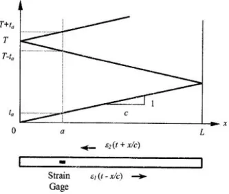
The Lagrange diagram of a single cylindrical bar could be as follows (figure 17 [17]), where a represents the position of the gauge:

Figure 17: Wave front traveling through a bar, shown in a Lagrange diagram

The line shows how much time it takes the wave front to travel to a certain point x on the bar. What the graphic doesn’t show is the actual duration of the wave. This means that, knowing the wave velocity 𝑐 = 𝐶0 and its travel duration t0, it is possible to determine the

best location for the gauges. If the strain gauge is too close to the free end, where the wave is being reflected, both the incident wave and the reflected wave could be measured at the same time, hence giving mixed results.

(43)

32 One must place the strain gauge far enough from the free end to have a fully reflected wave. It takes 𝑡𝑎 = 𝑎_𝑐 seconds to have a first reading on the gauge (the time it takes the

incident wave to reach the strain gage). Note that this reading is going to last t0 seconds.

A second reading is going to appear 𝑡𝑏 =2(𝐿−𝑎)_𝑐 seconds after the first one. If tb is shorter

than t0, there will be superposition of the incident and the reflected waves. Therefore, it is

required to have 𝐿0 < (𝐿 − 𝑎).

3.3.3 Compression versus Tension

It is important to remember that the concept chosen to adapt the compressive setup is the one suggested by Theodore Nicholas [18]. In order to get a tensile wave in the specimen, a collar is used to have the first compressive pulse completely transferred to the output bar, without affecting the specimen. The effect of the reflected tensile wave is what is going to be measured.

Figure 18: Collar type of tension SHPB

Since this setup is really similar to a compressive setup, it is possible to compare the Lagrange diagrams of both methods:

(44)

33

Figure 19: Lagrange diagrams for tension and compression SHPB

The left diagram of figure 19, picturing a compressive test (figure 19 a), shows that at the specimen/input bar interface, part of the pulse is reflected because of the impedance mismatch between the two mediums. The second reflection, at the end of the output bar, is of no interest since it does not provide any useful data that can be used to calculate the behavior of the specimen.

On the other hand, during a tensile test (figure 19 b), the reflection at the end of the output bar is important because it is actually the beginning of the test. The first part of the test, where the compressive wave is transmitted to the output bar, could be discarded, since no measurement is recorded during that time.

With respect to the tensile test (figure 19 b), consider only the part after the reflection of the compressive pulse, at the end of the output bar. It can be seen that the Lagrange diagram is then symmetric to that of the compressive test (figure 20).

Figure 20: Symmetry of a Lagrange diagram

The output bar of the compressive setup basically becomes the input bar of the tensile setup.

(45)

34 Moreover, the method proposed by Theodore Nicholas [18] allows use of the same pressure bars for both types of test. This means that, using the same materials, the wave speed c of the pressure bars does not change. Therefore, the pulse duration remains as t0=2L0/c0. This is why the development mentioned in section 2.2 is still valid and the

gauges do not need to be placed differently, depending on the type of experiments. Of course, this requires the apparatus to be symmetric. The two pressure bars must then be of same length and the gauges placed symmetrically on each side of the specimen.

Figure 19 b shows that there is a first reflection at the input bar/collar interface since the impedance between both bars does not match perfectly. It is important to make sure that there won’t be any superposition between this spurious reflected wave and the transmitted wave. This is easily verified using the development proposed in section 2.2. Figure 21 shows the same diagram as Figure 18, but this time the spurious wave is represented with a dash line and it is shown for a longer time.

Figure 21: Lagrange diagram showing the spurious wave

The spurious wave goes through the input bar strain gauge twice. There is a first reading after its reflection from the input bar/collar interface. Upon arrival at the free end of the input bar, the spurious wave is reflected a second time toward the 1st strain gauge.

The following provides the full development of the readings sequencing on both pressure bars after the impact. Times are calculated under the assumption that the setup is symmetric and neglecting the time it takes for the wave to travel along the specimen:

(46)

35 1. First reading on input bar: compressive initial pulse, at 𝑇0 = 𝑡𝑎 = 𝑎_𝑐

2. Second reading on input bar: spurious reflected tensile pulse at 𝑇1 = 𝑡𝑎+ 2𝑡𝑏 = 𝑎_𝑐 +2(𝐿−𝑎)_𝑐

3. Third reading on input bar: spurious reflected compressive pulse at 𝑇2 = 𝑡𝑎+ 2𝑡𝑏+ 2𝑡𝑎 =3𝑎_𝑐 +2(𝐿−𝑎)_𝑐

4. Fourth reading (recorded) on input bar: transmitted tensile pulse and reflected tensile spurious wave, at 𝑇3 = 3𝑡𝑎+4(𝐿−𝑎)_𝑐

5. First reading on output bar: compressive transmitted pulse, at 𝑇4 = 𝑡𝑎+2(𝐿−𝑎)_𝑐 = 𝑇1

6. Second reading (recorded) on output bar: reflected tensile pulse, at 𝑇5 = 3𝑡𝑎+2(𝐿−𝑎)_𝑐

7. Third reading (recorded) on output bar: reflected compressive pulse and transmitted spurious compressive wave, at 𝑇6 = 3𝑡𝑎+4(𝐿−𝑎)_𝑐

It is important to note that what needs to be recorded, in a tensile test, are points 4, 6 and 7. The other readings appear because the tensile load is indirect, with the first pulse being compressive and is therefore bypassed.

Considering the test is compressive, one can notice that the results come from the logic that no superposition is achieved if:

(𝑻𝟏− 𝑻𝟎) ≥ 𝒕𝟎 = 𝟐𝒕𝒃 ≥ 𝒕𝟎 (3.35)

If the same logic is applied for the spurious reflected waves in a tensile test, then there exists also 2 conditions:

(𝑻𝟑− 𝑻𝟏) ≥ 𝒕𝟎= (𝟐𝒕𝒂+ 𝟐𝒕𝒃) ≥ 𝒕𝟎 (3.36)

(47)

36 Therefore, if 𝑡𝑏≥ 𝑡0 was respected for the compressive test, then it is necessary that

(2𝑡𝑎+ 2𝑡𝑏) ≥ 𝑡0 is respected for the tensile test, since ta is non-negative. The second

condition of the tensile test is the same as the one for the compressive apparatus.

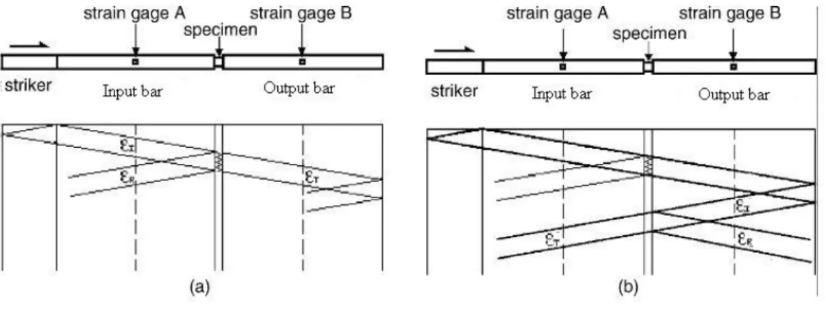
A problem of superposition is present at points 4 and 6. In figure 21, the dash lines, showing spurious waves, are merging with the full lines, showing the recorded pulse. This is caused by the setup symmetry and the most obvious way to solve this problem is to “remove” that symmetry, having bars of different lengths.

Figure 22 shows a new Lagrange diagram [8] where the pressure bars have different lengths. Even if figure 21 shows a longer input bar, this is not taken into consideration in the following equations.

Figure 22: Lagrange diagram for a non-symmetrical SHPB apparatus

The process described in section 3.2, can be written with no symmetry. 1. First reading on input bar: compressive initial pulse, at 𝑇0 = 𝑡𝑎𝑖𝑛 =

𝑎𝑖𝑛

𝑐

2. Second reading on input bar: spurious reflected tensile pulse at 𝑇1 = 𝑡𝑎𝑖𝑛 + 2𝑡𝑏𝑖𝑛 =

𝑎𝑖𝑛

𝑐 +

2(𝐿𝑖𝑛−𝑎𝑖𝑛)

𝑐

3. Third reading (recorded) on input bar: transmitted tensile pulse at 𝑇2 = 𝑡𝑎𝑖𝑛 + 2𝑡𝑏𝑖𝑛+ 2𝑡𝑏𝑜𝑢𝑡+ 2𝑡𝑎𝑜𝑢𝑡 = 𝑎𝑖𝑛 𝑐 + 2(𝐿𝑖𝑛−𝑎𝑖𝑛) 𝑐 + 2(𝐿𝑜𝑢𝑡−𝑎𝑜𝑢𝑡) 𝑐 + 2𝑎𝑜𝑢𝑡 𝑐

(48)

37

4. Fourth reading on input bar: reflected compressive spurious wave, at 𝑇3 = 3𝑡𝑎𝑖𝑛 + 2𝑡𝑏𝑖𝑛

5. First reading on output bar: compressive transmitted pulse, at 𝑇4 = 𝑡𝑎_𝑖𝑛 + 𝑡𝑏_𝑖𝑛+ 𝑡𝑏𝑜𝑢𝑡

6. Second reading (recorded) on output bar: reflected tensile pulse, at 𝑇5 = 𝑡𝑎𝑖𝑛+ 𝑡𝑏𝑖𝑛 + 𝑡𝑏𝑜𝑢𝑡+ 2𝑡𝑎𝑜𝑢𝑡

7. Third reading (recorded) on output bar: reflected compressive pulse, at 𝑇6 = 𝑡𝑎𝑖𝑛 + 𝑡𝑏𝑖𝑛+ 3𝑡𝑏𝑜𝑢𝑡+ 2𝑡𝑎𝑜𝑢𝑡

8. Fourth reading on input bar: transmitted compressive spurious wave, at 𝑇7 = 3𝑡𝑎𝑖𝑛 + 3𝑡𝑏𝑖𝑛+ 𝑡𝑏𝑜𝑢𝑡

Where:

𝑎𝑖𝑛 is the distance of the 1st strain gauge from the input bar free end

𝐿𝑖𝑛 is the length of the input bar

𝑎𝑜𝑢𝑡 is the distance of the 2nd strain gauge from the output bar free end

𝐿𝑜𝑢𝑡 is the length of the output bar

Most of the time in SHPB setups, the strain gauges are at the same distance from the specimen, therefore fixing (𝐿𝑖𝑛− 𝑎𝑖𝑛) = (𝐿𝑜𝑢𝑡− 𝑎𝑜𝑢𝑡) = 𝑏 and 𝑡𝑏𝑖𝑛 = 𝑡𝑏𝑜𝑢𝑡 = 𝑡𝑏. Here

are all the limitations for a tensile setup to obtain any superposition of the signals: •_(𝑇₁_{− 𝑇}₀_{) > 𝑡}₀ _{= 2𝑡}_𝑏_{≥ 𝑡}₀ •_(𝑇₂_{− 𝑇}₁_{) > 𝑡}₀ _{= �𝑡}_𝑎_𝑖𝑛_{+ 4𝑡}_𝑏_{+ 2𝑡}_𝑎_𝑜𝑢𝑡_{� − �𝑡}_𝑎_𝑖𝑛 _{+ 2𝑡}_𝑏_{� ≥ 𝑡}₀ _{= 2𝑡}_𝑏_{+ 2𝑡}_𝑎_𝑜𝑢𝑡 _{≥ 𝑡}₀ •_(𝑇₃_{− 𝑇}₂_{) > 𝑡}₀ _{= �3𝑡}_𝑎_𝑖𝑛 _{+ 2𝑡}_𝑏_{� − �𝑡}_𝑎_𝑖𝑛 _{+ 4𝑡}_𝑏_{+ 2𝑡}_𝑎_𝑜𝑢𝑡_{� ≥ 𝑡}₀ _{= 2𝑡}_𝑎_𝑖𝑛_{− 2𝑡}_𝑏₋ 2𝑡𝑎𝑜𝑢𝑡 ≥ 𝑡0 •_(𝑇₅_{− 𝑇}₄_{) > 𝑡}₀ _{= �𝑡}_𝑎_𝑖𝑛 _{+ 2𝑡}_𝑏_{+ 2𝑡}_𝑎_𝑜𝑢𝑡_{� − �𝑡}_𝑎_𝑖𝑛 _{+ 2𝑡}_𝑏_{� ≥ 𝑡}₀ _{= 2𝑡}_𝑎_𝑜𝑢𝑡 _{≥ 𝑡}₀ •_(𝑇₆_{− 𝑇}₅_{) > 𝑡}₀ _{= �𝑡}_𝑎_𝑖𝑛 _{+ 4𝑡}_𝑏_{+ 2𝑡}_𝑎_𝑜𝑢𝑡_{� − �𝑡}_𝑎_𝑖𝑛_{+ 2𝑡}_𝑏_{+ 2𝑡}_𝑎_𝑜𝑢𝑡_{� ≥ 𝑡}₀ _{= 2𝑡}_𝑏 _{≥ 𝑡}₀ •_(𝑇₇_{− 𝑇}₆_{) > 𝑡}₀ _{= �3𝑡}_𝑎_𝑖𝑛 _{+ 4𝑡}_𝑏_{� − �𝑡}_𝑎_𝑖𝑛 _{+ 4𝑡}_𝑏_{+ 2𝑡}_𝑎_𝑜𝑢𝑡_{� ≥ 𝑡}₀ _{= 2𝑡}_𝑎_𝑖𝑛₋ 2𝑡𝑎𝑜𝑢𝑡 ≥ 𝑡0

(49)

38 From the 4th_{condition, we can immediately find that:}

𝒂𝒐𝒖𝒕≥ 𝑳𝟎 (3.38)

Entering this new value in the 1st_{condition, we have}

𝑳𝒐𝒖𝒕≥ 𝟐𝑳𝟎 (3.39)

From the 3rd_{condition, we find that:}

𝒂𝒊𝒏 ≥ 𝟑𝑳𝟎 (3.40)

And again, including the last result in the 1st_{condition we conclude that:}

𝑳𝒊𝒏≥ 𝟒𝑳𝟎 (3.41)

In other words, a tensile setup like this one requires that the input bar be twice as long as the output bar, which is twice as long as the longest striker used. This means that the input bar must be at least 4 times the length of the striker. Nicholas et al. [18] also arrived at the same conclusion, using the same kind of experimental.

In the current compressive setup, both pressure bars are 800 mm long and the longest striker used has a length of 400 mm. On the other hand, supplied maraging steel bars are only available in sections of 914 mm, which leaves approximately 910 mm after machining. Considering this would be the longest pressure bar available, the longest striker that could be used would have to be 227.5 mm long.

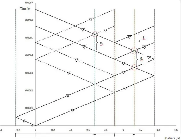
A Lagrange diagram of this situation is presented in the figure 23. For the sake of simplicity, the input bar is 900 mm instead of 910. As expected, the use of a 225 mm (4 times shorter than 900 mm) striker represents the limit of the system. Indeed, there are

(50)

39 locations on the diagram where the pulses “almost” intersect. These locations are circled in red on the figure.

In order to keep a safety margin, most simulations in this report are made with a 175 mm long striker.

(51)

40

Chapter 4:

(52)

41

The main software used to simulate SHPB tests, for this thesis work, is LS-Dyna. This section does not constitute a tutorial for LS-Dyna, but describes major elements that were taken into consideration to conduct the simulations.

When creating finite element models of parts interacting with each other, contact definition is crucial because it is known that the quality of a simulated contact is closely related to the quality of the mesh composing the parts. LS-Dyna’s default pre-processor, LS-Prepost, is not efficient enough regarding mesh controls and thus pre-processors are needed to create geometries and thus meshes.

Also, the first step in simulating the tensile results is to create a good compressive model. Previous work [19] shows the creation of a 2 dimension model for use with LS-Dyna. The methodology used was based on a 2D model and simulations were compared to experimental results.

4.2 Geometrical considerations

The parts of the existing compressive SHPB are as follows:

• 2 maraging steel pressure bars: dia 14.5 mm X 800 mm length • 1 maraging steel striker bar: dia 14.3 mm X 200 mm length • 1 aluminium 6061-T6 specimen: dia 10.5 mm X 5 mm length

In reality, the end of the striker bar has a 254 mm radius instead of being flat. This improves the contact between the striker and the input bar. For the simulations, because of the perfectly ortogonal contact, the striker is flat at both ends. Moreover, the striker diameter is slightly smaller than 14.5 mm to fit the air gun bore. For the simulation, diameter was to be exactly 14.5 mm, again given that the contact is orthogonal when the striker hits the incident bar.

4.3 Mesh considerations

The model consists of 4 basic components in the case of compression SHPB and 5 in the case of the tension SHPB, because of the added collar. The parts are:

(53)

42 • Specimen

• Input bar • Output bar • Striker

• Collar (in the case of the tension system)

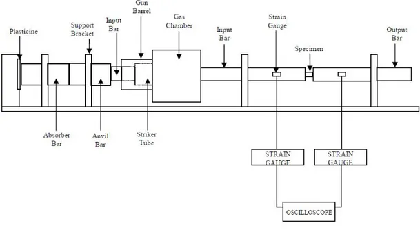
Figure 24 : Typical SHPB setup

All the parts listed are in contact at some point during experiment and, therefore, mesh definition is extremely crucial. In FEA analysis, the quality of the contact between two parts is closely related to the mesh. It is important that parts that are in contact have coincident nodes at contact interface. Figure 25 shows the elements at the extremities of the input and striker bars, with the nodes being coincident.

Figure 25: Nodes correspondence at bars extremities

4.4 Material considerations

The material constitutive relations that are used for both compression and tension models are:

• Elastic (for the bars)

(54)

43 • Johnson-Cook with damage (for the sample in tension)

The plastic-kinematic constitutive model of LS-Dyna (see section 4.4.2) is used in compression case in order to compare with a previously done study conducted by A. Bouamoul study [19]. The Johnson-Cook model with damage law is used to simulate the deformation of the specimen until failure.

4.4.1 Elastic (Hooke) law

The Hooke’s law is used as a constitutive model in the simulation of the pressure bars, the striker and the collar behavior. Since all of those components are not to be deformed plastically, this simple law is sufficient for the model.

As presented by Mase [20], the general elastic relation is

𝝈𝒊𝒋 = 𝑪𝒊𝒋𝒌𝒎𝜺𝒌𝒎 (4.1)

This relation links strains to stresses and the fourth-order tensor of the previous equation is given by:

𝑪𝒊𝒋𝒌𝒎= 𝝀𝜹𝒊𝒋𝜹𝒌𝒎+ 𝝁�𝜹𝒊𝒌𝜹𝒋𝒎+ 𝜹𝒊𝒎𝜹𝒋𝒌�

+ 𝜷�𝜹𝒊𝒌𝜹𝒋𝒎− 𝜹𝒊𝒎𝜹𝒋𝒌�

(4.2)

For an isotropic material, equations 4.1 and 4.2 reduce to

𝝈𝒊𝒋 = 𝝀𝜹𝒊𝒋𝜺𝒌𝒌+ 𝟐𝝁𝜺𝒊𝒋 (4.3)

where 𝜆 and 𝜇 are Lamé constants. The well-known Young modulus and Poisson ratio can both be expressed as a function of in term of Lamé constants:

𝑬 = 𝝁(𝟑𝝀 + 𝟐𝝁)_{𝝀 + 𝝁} (4.4)

(55)

44

4.4.2 Plastic-kinematic law

This constitutive model is suited for isotropic material with kinematic hardening. Strain rate dependency is not taken into account here as this as little effects on the aluminum response. Moreover, to consider only isotropic hardening, parameter 𝛽 must be set to 1 in LS-Dyna.

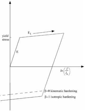
In figure 26, hardening is modeled simply as linear isotropic hardening:

Figure 26: Linear kinematic hardening representation

To account for plasticity, a tangent modulus is required, as well as the yield stress. It is not necessary to model kinematic hardening as it is mostly suited for cyclic loading. Therefore, one could think of this law as linear until the yield stress is reached, followed by another linear law until failure has occured.

4.4.3 Johnson-Cook material model with a damage law

As mentioned earlier, this law is often used for ductile materials when strain rate dependency and damage are to be considered. This means that, unlike the plastic

(56)

45 kinematic law shown above, here strain rate effects and damage evolution until failure, instead of linear strain increase until the limit is reached.

As presented by LS-Dyna Keyword User Manual [21], Johnson-Cook expresses the flow stress as follows:

𝝈𝒚= �𝑨 + 𝑩𝜺𝒑�𝒏�(𝟏 + 𝑪 𝐥𝐧 𝜺̇∗)(𝟏 − 𝑻∗𝒎) (4.6)

Where A, B, C, m and n are material constants. 𝜀𝑝̅_{is the effective plastic strain}

𝜀̇∗_{is the effective total strain rate normalized to static threshold rate (the}

quasi-static threshold rate is the strain rate under which no rate effects are apparent). and 𝑇∗ ₌ 𝑇−𝑇𝑟𝑜𝑜𝑚

𝑇𝑚𝑒𝑙𝑡−𝑇𝑟𝑜𝑜𝑚

For damage, the total strain at fracture is given by:

𝜺𝒇 = �𝑫𝟏+ 𝑫𝟐𝒆𝑫𝟑𝝈∗�(𝟏 + 𝑫𝟒𝐥𝐧 𝜺̇∗)(𝟏 + 𝑫𝟓𝑻∗) (4.7)

Where D1 to D5 are material damage parameters.

Fracture occurs when the overall cumulated damage parameter reaches the value 1.

𝑫 = �∆𝜺_𝜺𝒑�

𝒇 (4.8)

4.5 Conclusion

The main considerations taken into account when creating the finite elements model are: • Using the same geometry as the one currently in place at DRDC laboratories. • Having a good quality mesh, especially at contact zone interfaces

For tensile simulations, the Johnson-Cook with damage law is what is commonly used when modeling metals under high rates of strain.

(57)

46

Chapter 5:

(58)

47

In order to create a tensile Hopkinson pressure bar apparatus, based on a compressive setup, a 3 dimensions simulation model needs to be created. With this model, it is possible to predict what the results of the tensile experiments are going to be and the design can therefore be adjusted as a consequence.

The first step in simulating the tensile results is to create a good compressive model. A previous report [19] shows the creation of a two dimensional model on LS-Dyna.

The current paper shows the simulation, in three dimensions, of the compressive apparatus. The methodology used was based on the 2D model and other experimental results. This was done in order to have a good starting point for the 3D tension model. It was decided to have the tension model in 3D, as it is more versatile.

5.2 Model creation in LS-Dyna

The materials constitutive laws used in the 3D model are the same as those used in the 2D model [19] (see table 4):

Table 4: Aluminum and Steel properties

Maraging Steel Aluminum 6061-T6

Constitutive law = Elastic Constitutive law = Plastic kinematic Young Modulus = 182.1 GPa Young Modulus = 73.08 GPa

Density = 8064 kg/m3 _{Density = 2690 kg/m}3

Poisson ratio = 0.3 Poisson ratio = 0.33

Elastic limit = 335 MPa