HAL Id: hal-02166675
https://hal.archives-ouvertes.fr/hal-02166675
Submitted on 27 Jun 2019
HAL is a multi-disciplinary open access
archive for the deposit and dissemination of
sci-entific research documents, whether they are
pub-lished or not. The documents may come from
teaching and research institutions in France or
abroad, or from public or private research centers.
L’archive ouverte pluridisciplinaire HAL, est
destinée au dépôt et à la diffusion de documents
scientifiques de niveau recherche, publiés ou non,
émanant des établissements d’enseignement et de
recherche français ou étrangers, des laboratoires
publics ou privés.
Programming the Demirci-Selçuk Meet-in-the-Middle
Attack with Constraints
Danping Shi, Siwei Sun, Patrick Derbez, Yosuke Todo, Bing Sun, Lei Hu
To cite this version:
Danping Shi, Siwei Sun, Patrick Derbez, Yosuke Todo, Bing Sun, et al.. Programming the
Demirci-Selçuk Meet-in-the-Middle Attack with Constraints. ASIACRYPT 2018, Dec 2018, Brisbane,
Aus-tralia. �hal-02166675�
Programming the Demirci-Sel¸
cuk
Meet-in-the-Middle Attack with Constraints
Danping Shi1,2, Siwei Sun1,2,3?, Patrick Derbez4, Yosuke Todo5
Bing Sun6, and Lei Hu1,2,3
1 State Key Laboratory of Information Security, Institute of Information
Engineering, Chinese Academy of Sciences, China
2 Data Assurance and Communication Security Research Center,
Chinese Academy of Sciences, China
3 School of Cyber Security, University of Chinese Academy of Sciences, China
{shidanping, sunsiwei, hulei}@iie.ac.cn
4 Univ Rennes, CNRS, IRISA, France [email protected]
5
NTT Secure Platform Laboratories, Japan [email protected]
6 College of Liberal Arts and Sciences, National University of Defense Technology,
China happy [email protected]
Abstract. Cryptanalysis with SAT/SMT, MILP and CP has increased in popularity among symmetric-key cryptanalysts and designers due to its high degree of automation. So far, this approach covers differential, linear, impossible differential, zero-correlation, and integral
cryptanaly-sis. However, the Demirci-Sel¸cuk meet-in-the-middle (DS-MITM) attack
is one of the most sophisticated techniques that has not been automated with this approach. By an in-depth study of Derbez and Fouque’s work on DS-MITM analysis with dedicated search algorithms, we identify the crux of the problem and present a method for automatic DS-MITM at-tack based on general constraint programming, which allows the crypt-analysts to state the problem at a high level without having to say how it should be solved. Our method is not only able to enumerate distin-guishers but can also partly automate the key-recovery process. This approach makes the DS-MITM cryptanalysis more straightforward and easier to follow, since the resolution of the problem is delegated to off-the-shelf constraint solvers and therefore decoupled from its formulation. We apply the method to SKINNY, TWINE, and LBlock, and we get the currently known best DS-MITM attacks on these ciphers. Moreover, to demonstrate the usefulness of our tool for the block cipher designers, we exhaustively evaluate the security of 8! = 40320 versions of LBlock in-stantiated with different words permutations in the F functions. It turns out that the permutation used in the original LBlock is one of the 64 permutations showing the strongest resistance against the DS-MITM at-tack. The whole process is accomplished on a PC in less than 2 hours. The same process is applied to TWINE, and similar results are obtained.
Keywords: Demirci-Sel¸cuk meet-in-the-middle attack, Automated
crypt-analysis, Constraint programming, MILP ?
1
Introduction
Cryptanalysis of block ciphers is a highly technical, time consuming and error-prone process. On the one hand, the attackers have to perform a variety of cryptanalytic techniques, including differential attack [1], linear attack [2], inte-gral attack [3–5], etc., to see which technique leads to the best attack. On the other hand, the designers need to repeat all these different attacks again and again to identify the optimal choices of parameters and building blocks which meet the security and implementation requirements. Therefore, automatic tools are indispensable to the community, which significantly reduce the manual work and make a thorough exploration of the design/analysis space possible.
One paradigm for automatic symmetric-key cryptanalysis getting increasing popularity in recent years is to model the problem by means of constraints, which includes the methods based on SAT/SMT (satisfiability modulo theory) [6–8], MILP (mixed-integer linear programming) [9–13], and classical constraint pro-gramming [14, 15]. In this paper, these methods are collectively referred to as the general constraint programming (CP) based approach, or just CP based ap-proach for short. So far, the CP based apap-proach covers a wide range of symmetric-key cryptanalysis techniques. For instance, we can determine the minimum num-ber of differentially or linearly active S-boxes of a block cipher with MILP [9]; we can search for actual differential characteristics, linear characteristics, and inte-gral distinguishers with SAT/SMT, MILP or classical constraint programming [8, 10, 11, 14]; and we can search for impossible differentials and zero-correlation linear approximations [12, 16] in a similar way.
Compared with search algorithms implemented from scratch in general pur-pose programming languages [17–24], the CP based approach allows the crypt-analysts to state the problem very naturally, and at a high level without having to say how it should be solved. The resolution of the problem is delegated to generic solvers, and therefore decoupled from the formulation of the problem. As Eugene C. Freuder stated [25]: Constraint programming represents one of the closest approaches computer science has yet made to the Holy Grail of program-ming : the user states the problem, the computer solves it.
However, the Demirci-Sel¸cuk meet-in-the-middle attack (DS-MITM) attack
[26], introduced by Demirci and Sel¸cuk at FSE 2008 to attack the famous Ad-vanced Encryption Standard (AES) [27], is one of the cryptanalytic techniques which has not been automated with general constraint programming due to its extraordinary sophistication. After a series of improvements of the attack
with various creative techniques [28–32], theDS-MITM attack reaches the best
known attack on 7-round AES-128, 9-round AES-256 and 10-round AES-256 in the single-key model. The attack has been applied to several specific block ciphers [33–36] as well as on generic balanced Feistel constructions [37]. Most recently, Guo et al. show generic attacks on unbalanced Feistel ciphers based on
theDS-MITM technique which penetrate a large number of rounds of some
spe-cific class of unbalanced Feistels [38]. Note that despite sharing the same name with the traditional MITM attacks in some literature (the attacks on some block
ciphers [39, 40] and on a number of hash functions, e.g. [41, 42]), theDS-MITM attack concerned in this paper follows a different and a more complex strategy.
Related work and our contribution. In [30, 31], Derbez and Fouque presented
a tool implemented in C/C++ for finding theDS-MITM attack with dedicated
search algorithm. In this paper, we present the first CP-based tool for finding
theDS-MITM attack automatically. Our approach is based on a novel modelling
technique in which we introduce several different types of variables for every input/output word of all operations, and impose constraints on these variables such that from a solution of these variables satisfying all the constraints we can
deduce aDS-MITM distinguisher or DS-MITM attack.
Compared with Derbez and Fouque’s tool [30, 31] which was implemented in the general purpose programming language C/C++, the CP based method allows the cryptanalysts to state the problem at a high level very naturally, without considering how to maintain the relationships between the variables explicitly with dedicated algorithms. Therefore, our tool should be very useful in fast prototyping in the process of block cipher design.
In [43], Lin et al. modeled the problem of searching for DS-MITM
distin-guishers as an integer programming model. However, their integer programming model is incomplete and is solved by a dedicated search algorithm. Secondly, Lin et al. ’s work only focuses on the distinguisher part. Our CP based approach can not only enumerate distinguishers but also partly automate the key-recovery process of the attack. Moreover, by applying our CP based approach to LBlock, the same cipher targeted in [43], we show it finds better distinguishers as well as better attacks. To demonstrate the effectiveness of our approach, we apply it to SKINNY [44], TWINE [45], and LBlock [46]. We produce so far the best DS-MITM attacks on these well-known ciphers automatically.
For LBlock, we can not only find an 11-roundDS-MITM distinguisher which
is 2 rounds longer than the one(s) presented in [43], but also construct the
firstDS-MITM attack on 21-round LBlock. We also rediscover the same attack
on TWINE-128 given in [34], and identify the first DS-MITM attack on
20-round TWINE-80. In addition, we report the first concrete DS-MITM analysis
of SKINNY. A remarkable fact is that our tool identify an 10.5-roundDS-MITM
distinguisher in a few seconds, while its designers expect an upper-bound of 10 rounds against such distinguishers in [44]. A summary of these results are given in Table 1.
We also show how helpful our tool can be in the block cipher design process by searching for the best choices of block shuffles in LBlock and TWINE. We scan over 40320 variants of LBlock, and 887040 variants of TWINE. We iden-tify permutations which are potentially stronger than the permutations in the original designs. We make the source code of this work publicly available at
https://github.com/siweisun/MITM.
In addition, all supplementary materials referred later on are provided in an
Table 1: A summary of the results. Though the focus of this paper is the DS-MITM attack, we also list other types of attacks which achieve currently known
best results against the ciphers targeted. For theDS-MITM attack, the number of
rounds attacked is presented in the form of a+b, where a shows how many rounds
are covered by the underlyingDS-MITM distinguisher, while b is the number or
outer rounds added when performing a key-recovery attack. Therefore, b = 0 indicates a distinguishing attack.
Target Rounds Time Data Memory Method Ref
LBlock 11 + 10 270.20 248CP 261.91 DS-MITM Sect. 7.2 9 + 0 274.5 − − DS-MITM Dist. [43] 23 274.5 259.5CP 274.3 ID [47] 23 275.36 259CP 274 ID [48] 23 272 262.1Kp 260 MultiD ZC [47] 23 276 262.1Kp 260 MultiD ZC [49] TWINE80 11 + 9 277.44 232CP 282.91 DS-MITM Sect. 7.3 23 279.09 257.85CP 284.06 ID [50] 23 273 262.1KP 260 MultiD ZC [47] TWINE128 11 + 14 2124.7 248CP 2109 DS-MITM? [34] 25 2124.5 259.1CP 278.1 ID [34] 25 2119 262.1KP 260 MultiD ZC [47] 25 2122.12 262.1KP 260 MultiD ZC [49] SKINNY-128-384 10.5 + 11.5 2 382.46 296CP 2330.99 DS-MITM Sect. 7.1 11 + 11 2373.48292.22CP 2147.22 ID [51] ? We find the attacks with the same complexity.
Organization.In Sect. 2, we give the notations used in this paper. An
intro-duction of the DS-MITM attack is presented in Sect. 3. We show the general
principle of how to model theDS-MITM attack in Sect. 4, and subsequently in
Sect. 5 the technical detail of the modelling method is given. Sect. 6 discusses how to use our method in practice. In Sect. 7, we apply our approach to SKINNY, TWINE, LBlock, AES, ARIA, and SIMON. In Sect. 8, we discuss how to use our
tool to find high-quality building blocks (with respect to theDS-MITM attack)
in the process of block cipher design. Sect. 9 is the conclusion.
2
Notations
An n-bit state state with n = cnc is alternatively regarded as a sequence
(state[0], state[1],· · · , state[nc− 1]) of nc c-bit words. Let A = [j0, j1,· · · , js−1]
be an ordered set of integers such that 0≤ j0<· · · < js−1< nc. Then state[A]
is used to represent state[j0]|| · · · ||state[js−1], where state[j] is the j-th c-bit word
Definition 1. A set {P0,· · · , PN−1} ⊆ Fcnc
2 = Fn2 of N = 2sc n-bit values for
state is a δ(A)-set for state with A = [k0, k1,· · · , ks−1] if P0[A] ⊕ Pj[A] = j
(1≤ j < N), and Pi[k] = Pj[k] for all i, j
∈ {0, · · · , N −1} and k /∈ A. That is,
{P0,
· · · , PN−1} traverse the s c-bit words specified by A while share the same
value in other word positions.
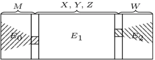
An r-round iterative block cipher E with r = r0+ r1+ r2, depicted in Fig. 1,
is a keyed permutation which transforms an n-bit state state0into state2rstep by
step with nonlinear and linear operations. In our indexing scheme, as illustrated
in Fig. 1, state2kis the input state of round k, state2k+1is the output state of the
nonlinear operation of round k, and state2(k+1) is the output of round k or the
input of round k+1 for k∈ {0, · · · , r0+r1+r2−1}. For the sake of simplicity and
concreteness, we will conduct the discussion based on Fig. 1, which visualizes the structure of a common SP cipher. Without loss of generality, we assume that the key addition is performed after the linear layer L as illustrated in Fig. 1. The basic rule is that we should always introduce a new state for the direct input to the nonlinear layer. For example, if the key addition is performed in between
state2i and the NL operation, then a new state (representing the direct input to
NL) should be introduced in between the key addition and the NL operation, and the original state may be omitted (regarding the new state as an output obtained by masking the output of the previous round with the subkey).
Note that though our discussion are based on a SP cipher illustrated in Fig. 1, the ideas and techniques presented in this paper are general enough to be applied to other structures, such as Feistel and Generalized Feistel structures.
For convenience, a δ(A)-set {P0,· · · , PN−1} is denoted by P
δ(A), and let
∆E(Pδ(A),B) be the sequence [C0[B]⊕C1[B], · · · , C0[B]⊕CN−1[B]], where Ci=
E(Pi) andB = [j
0,· · · , jt−1] such that 0≤ j0<· · · < jt−1 < nc.
Let P , P0 ∈ Fn
2 be two values of state0 shown in Fig. 1, which are often
regarded as plaintexts since state0 is the input of the encryption algorithm. The
value P creates a series of intermediate values during the encryption process. We
define P (statei) as the intermediate value at stateicreated by the partial
encryp-tion of P . Sometimes we only care about the value of P (statei) at some specified
word positions indexed by an ordered set I, which is denoted by P (statei[I]).
We define P⊕ P0(statei) and P⊕ P
0
(statei[I]) to be the intermediate differences
P (statei)⊕ P
0
(statei) and P (statei[I]) ⊕ P
0
(statei[I]) respectively. Let C and
C0 be the ciphertexts of P and P0. An intermediate value can also be regarded
as the result of a partial decryption of the ciphertext C. Therefore, we define
C(statei), C(statei[I]), C ⊕ C
0
(statei), and C⊕ C
0
(statei[I]) similarly. Note that
in the above notations, the intermediate values or differences of intermediate val-ues are specified with respect to some plaintexts or ciphertexts. We may as well
specify them with respect to some intermediate values, say Q = P (statej) and
Q0 = P0(statej). Hence, we may have notations such as Q(statei), Q(statei[I]),
Q⊕ Q0(statei), and Q⊕ Q
0
(statei[I]), whose meanings should be clear from the
context.
To make the notation succinct, if not stated explicitly, we always assume
Plaintext ¯ A state0 NL state1 L k0 state2 E0 (0→ · · · → r0 − 1) Involved Key: kE0
.. . state2(r0−1) NL state2(r0−1)+1 L kr0−1 A state2r0 NL state2r0+1 L kr0 state2(r0+1) E1 (r0 → · · · → r0 + r1 − 1) .. . state2(r0+r1−1) NL state2(r0+r1−1)+1 L kr0+r1−1 B state2(r0+r1) NL state2(r0+r1)+1 L kr0+r1 state2(r0+r1+1) E2 (r0 + r1 → · · · → r0 + r1 + r2 − 1) Involved Key: kE2
.. . state2(r0+r1+r2−1) NL state2(r0+r1+r2−1)+1 L kr0+r1+r2−1 state2(r0+r1+r2) Ciphertext
Fig. 1: An r-round SP block cipher E = E2◦ E1◦ E0with r = r0+ r1+ r2, whose
round function consists of a layer of nonlinear operation and a layer of linear
operation. ADS-MITM key-recovery attack is performed based on a DS-MITM
distinguisher placed at E1. A more detailed explanation of this figure will be
given in Sect. 3.2.
a sequence of n bits or a sequence of nc c-bit words. Moreover, we make the
following assumption which is very natural for a block cipher.
Assumption 1 Let the nonlinear layer in Fig. 1 be a parallel application of
nc c× c invertible S-boxes, and I = [j : Q ⊕ Q
0
(state2k[j]) 6= 0, 0 ≤ j <
nc] be an ordered set, where Q and Q
0
are two values for state2k. If we know
the value of Q(state2k[I]), then we can derive the value of Q ⊕ Q
0
with the knowledge of Q⊕ Q0(state2k[I]). Similarly, we can derive the value of
Q⊕ Q0(state2k) with the knowledge of Q(state2k+1[I]) and Q ⊕ Q
0
(state2k+1[I]).
In other words, we can derive the value of the output/input differences if we know the value of input/output values and differences at the active positions.
3
The Demirci-Sel¸
cuk Meet-in-the-Middle Attack
3.1 The DS-MITM Distinguisher
The DS-MITM attack relies on a special differential-type distinguisher.
Com-pared with ordinary differential distinguishers, theDS-MITM distinguishers
gen-erally lead to much stronger filters.
Let F be a keyed permutation, and Qδ(A)={Q0,· · · , QN−1} be a δ(A)-set
for the input state of F . If F is a random permutation, then it can be shown
that there are (2ct)2cs
−1 possibilities for ∆
F(Qδ(A),B). But for a block cipher
F , it is possible that the sequence ∆F(Qδ(A),B) can be fully determined with
the knowledge of d c-bit words. For instance, from the values of one internal state and the master key one can derive the values for all the internal states.
Therefore, given Qδ(A), we can get at most 2cdpossible cases of ∆F(Qδ(A),B) by
traversing the d c-bit words. We call d the (A, B)-degree of F , which is denoted
by DegF(A, B), or simply Deg(A, B) if F can be inferred from the context. If
DegF(A, B) = d is small enough such that λ = 2cd/(2ct)2
cs
−1 = 2c(d−t·(2cs
−1))<
1, or d < t· (2cs− 1), then we can use this property as a distinguisher and
construct a key-recovery attack on F . Therefore, aDS-MITM distinguisher of a
keyed permutation F can be regarded as a tuple (A, B, DegF(A, B)).
3.2 Key Recovery Attack based on DS-MITM Distinguisher
We now describe how a key-recovery attack can be performed with aDS-MITM
distinguisher. This part should be read while referring to Fig. 1.
As shown in Fig. 1, we divide the target cipher E into 3 parts: E0, E1, and
E2, where Ei is a keyed permutation with ri rounds. As depicted in Fig. 1, E0
covers rounds (0→ · · · → r0−1), E1covers rounds (r0→ · · · → r0+ r1−1), and
E2 covers rounds (r0+ r1→ · · · → r0+ r1+ r2− 1). According to our indexing
scheme, as illustrated in Fig. 1, state0 is the input state of E0; state2r0 is the
output state of E0which is also the input state of E1; state2(r0+r1)is the output
of E1 or the input of E2; finally, state2(r0+r1+r2) is the output of E2.
In the attack, we place aDS-MITM distinguisher (A, B, DegE1(A, B)) at E1,
and prepare a δ( ¯A)-set Pδ( ¯A) of chosen plaintexts for state0, where ¯A is the
ordered set of integers k (0≤ k < nc) such that V0⊕ Vj(state0[k])6= 0 for some
δ(A)-set Vδ(A) ={V0,· · · , VN−1} for state2r0 (the input state of E1) and some
j∈ {0, · · · , N − 1}. Note that ¯A can be obtained by propagating the differences
created by Vδ(A) for state2r0 (the input of E1) reversely against E0.
Then we select an arbitrary plaintext P0 from P
δ( ¯A), and guess the secret
key information kE0 ∈ F
e0
that Qδ(A)={Q0,· · · , QN−1} where Qj = E0(Pj) forms a δ(A)-set for state2r0.
Finally, we guess the secret key information kE2∈ F
e2
2 involved in E2with which
we can determine the sequence
∆E1(Qδ(A),B) = [C 0 ⊕ C1(state 2(r0+r1)[B]), · · · , C 0 ⊕ CN−1(state 2(r0+r1)[B])]
by partial decryption with E2, where Cj = E(Pj).
If the resulting sequence is not one of the possible ∆E1(Qδ(A),B) sequences
which can be determined with the DegE1(A, B) = d c-bit parameters, the guesses
of kE0 and kE2 are certainly incorrect and therefore rejected. Similar to [52], we
adopt the notion of|kE0∪kE2| to represent the log of the entropy of the involved
secret key bits in the outer rounds from an information theoretical point of view.
3.3 Complexity Analysis
Offline phase. Store all the 2cdpossibilities of the sequence ∆
E1(Qδ(A),B) in a
hash table. The time complexity is 2cd
·2cs
·ρE1CE , and the memory complexity
is (2cs
− 1) · ct · 2cdbits, where C
E is the time complexity of one encryption with
E, and ρE1 is typically computed in literature as Deg(A, B) divided by the total
number of S-boxes in E.
Online phase. For each of the 2|kE0∪kE2| possible guesses, if the resulting
se-quence ∆E1(Qδ(A),B) is not in the hash table precomputed, then the guess under
consideration is certainly not correct and is discarded. The time complexity of
this step is 2|kE0∪kE2|·2sc·ρE0∪E2CE, where ρE0∪E2is typically computed as the
number of S-boxes involved in the outer rounds divided by the total number of
S-boxes in E. After this step, the 2|kE0∪kE2|key space is reduced approximately
to λ· 2|kE0∪kE2|, where λ = 2c(d−t·(2cs−1))
.
4
Modelling the DS-MITM Attack with Constraints: A
High Level Overview
In this section, we give a high level overview of our modelling method with the aid of Fig. 1 and Fig. 2, which serves as a road map for the next section (Sect. 5), where the technical details are presented. To model the attack with constraint
programming (CP) for the cipher E = E2◦ E1◦ E0shown in Fig. 1, we proceed
as the following steps.
Step 1. Modelling the distinguisher part
• Introduce three types (X, Y , and Z) of 0-1 variables for each word of the
states state2r0,· · · , state2(r0+r1) involved in E1. We denote the sets of all
type-X, type-Y and type-Z variables by Vars(X), Vars(Y ) and Vars(Z), re-spectively.
• Introduce a set of constraints over Vars(X) to model the propagation of the forward differential, and introduce a set of constraints over Vars(Y ) to model the backward determination relationship.
• Impose a set of constraints on Vars(Z) such that a type-Z variable for statei[j]
is 1 if and only if the type-X and type-Y variables for statei[j] are 1
Remark 1. Under the above configuration, every instantiation of the variables
in Vars(X), Vars(Y ), and Vars(Z) corresponds to a potential DS-MITM
distin-guisher. Therefore, all distinguishers can be enumerated with the above model. Also note that the key addition can be omitted while searching for distinguishers if it does not affect the propagation of the forward differential and backward de-termination relationship. This is the case for all the examples presented in this paper, where key additions are only involved in computing the actual complex-ities.
Step 2. Modelling the outer rounds
• Introduce a type-M variable for each word of the states state0,· · · , state2r0
involved in E0, and impose a set of constraints over Vars(M ) to model the
backward differential. Note that there are both type-X and type-M variables
for state2r0. We require that the corresponding type-X and type-M variables
for each of the nc words of state2r0 are equal.
• Introduce a type-W variable for each word of the states state2(r0+r1), · · · ,
state2(r0+r1+r2)involved in E2, and impose a set of constraints over Vars(W )
to model the forward determination relationship. Note that there are both
type-Y and type-W variables for state2(r0+r1). We require that the
corre-sponding type-Y and type-W variables for each of the ncwords of state2(r0+r1)
are equal.
Remark 2. Every solution of Vars(M ) and Vars(W ) helps us to identify the
information that needs to be guessed in the outer rounds, which will be clearer in the following. E0 M E1 X, Y, Z E2 W
Fig. 2: A high level overview of the modelling method forDS-MITM attack
The overall modelling strategy is depicted in Fig. 2. In summary, given a full solution of the variables such that all constraints are fulfilled, we can extract the following information
• A : The variables in Vars(X) for state2r0 whose values are 1 indicate A;
• B : The variables in Vars(Y ) for state2(r0+r1)whose values are 1 indicateB;
• DegE1(A, B) : The variables in Vars(Z) for state2j, r0 ≤ j < r0+ r1 whose
values are 1 indicate DegE1(A, B);
• ¯A and guessed materials in E0 : The variables in Vars(M ) whose values are
1 indicate ¯A and guessed materials in E0which tells us how to prepare the
• Guessed materials in E2 : The variables in Vars(W ) whose values are 1
indicate the Guessed materials in E2 with which we can derive the sequence
of differences at state2(r0+r1)from the ciphertexts.
Together this information forms aDS-MITM attack on E. Note that the guessed
materials in E0and E2still need to be converted to guessed key materials, which
can be done manually or automatically fairly straightforwardly.
According to the semantics of Vars(Z), if we draw the propagation patterns of Vars(X) and Vars(Y ) in two figures, then the propagation pattern of Vars(Z) can be obtained by superposition of the two figures. Therefore, the key to understand
the details of the modelling of DS-MITM attack is the so-called
forward/back-ward differentialand forward/backward determination relationship. To make the
description succinct and without loss of generality, we introduce the concepts based on a 5-round keyed permutation shown in Fig. 4 and Fig. 6. We will also give two concrete examples of the forward differential and backward determina-tion of a 3-round toy SPN block cipher with 32-bit (4-byte) block size. The round function shown in Fig. 3 of the toy cipher consists of an S-box layer (a parallel
ap-plication of four 8× 8 Sboxes), and a linear layer L with yi=Lj∈{0,1,2,3}−{i}xj
for i∈ {0, 1, 2, 3}. S S S S x0 x1 x2 x3 L AK y0 y1 y2 y3
Fig. 3: The round function of the toy cipher
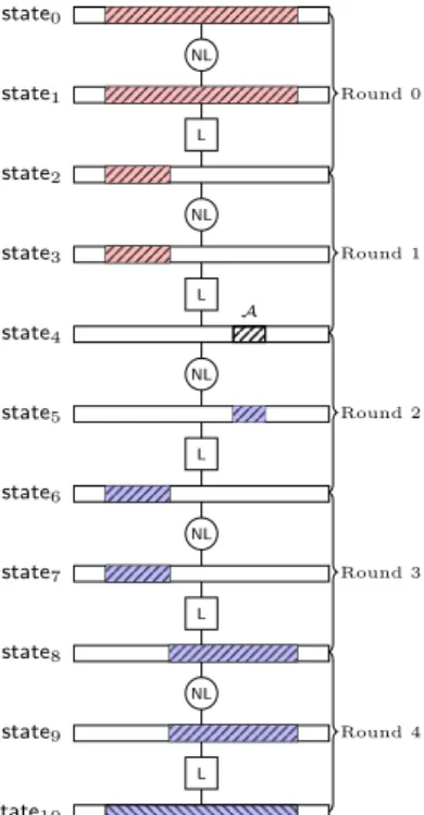
4.1 Forward Differential and Backward Differential
As shown in Fig. 4, given a set Qδ(A) of N values {Q0,· · · , QN−1} for state4
which forms a δ(A) set for the input state of round 2. For every word statei[j] (4≤
i ≤ 10, 0 ≤ j < nc), we introduce a 0-1 variable Xi[j]. We say that the set of
0-1 variables {Xi[j] : 4≤ i ≤ 10, 0 ≤ j < nc} models the forward differential of
Qδ(A) in rounds (2→ 3 → 4) if the following conditions are satisfied.
- Conditions for state4(the starting point of the forward differential, which is
also the input of round 2) :∀j ∈ A, X4[j] = 1 and∀j /∈ A, X4[j] = 0
- Conditions for rounds (2→ 3 → 4): Xi[j] = 0 (5 ≤ i ≤ 10, 0 ≤ j < nc) if
and only if∀Qk
∈ Qδ(A), Q0⊕ Qk(statei[j]) = 0
Similarly, as depicted in Fig. 4, we say that the set of variables{Xi[j] : 0≤
i≤ 4, 0 ≤ j < nc} models the backward differential of Qδ(A) in rounds (1→ 0)
- Conditions for state4 (the starting point of the backward differential, which
is also the output of round 1):∀j ∈ A, X4[j] = 1 and∀j /∈ A, X4[j] = 0
- Conditions for rounds (1→ 0): Xi[j] = 0 (0≤ i < 4, 0 ≤ j < nc) if and only
if∀Qk ∈ Qδ(A), Q0⊕ Qk(statei[j]) = 0 NL L state0 state1 Round 0 NL L state2 state3 Round 1 NL L state4 state5 Round 2 NL L state6 state7 Round 3 NL L state8 state9 Round 4 state10 A
Fig. 4: Forward/backward differential illustrated on a 5-round keyed permutation
Let us give a concrete example. LetA = [3] and Qδ(A)={(0, 0, 0, x) ∈ (F82)4:
x∈ F8
2}. Then the set of variables Xi[j] with 0≤ i ≤ 6 and 0 ≤ j < 4 shown in
Fig. 5 models forward differential of Qδ(A) in rounds (0→ 1 → 2) if we impose
the following constraints on Xi[j]. Since the values in Qδ(A) are active at the
third byte, we have X0[0] = X0[1] = X0[2] = 0, X0[3] = 1. For the S-layers in the
toy cipher, we have X2i[j] = X2i+1[j], 0≤ i ≤ 2, 0 ≤ j < 4. For the linear layers,
we enforce 3X2(i+1)[j]− X2i+1[j + 1]− X2i+1[j + 2]− X2i+1[j + 3]≥ 0 to ensure
that X2(i+1)[j] will be equal to 1 when any one of X2i+1[j + 1], X2i+1[j + 2],
X2i+1[j + 3] is 1. We also add the constraint
X2i+1[j + 1] + X2i+1[j + 2] + X2i+1[j + 3]− X2(i+1)[j]≥ 0
to dictate that X2(i+1)[j] must be 0 when all of X2i+1[j + 1], X2i+1[j + 2],
X2i+1[j + 3] are 0, where 0≤ i ≤ 2, 0 ≤ j < 4 and the indexes are computed
modulo 4. With these constraints, the Xi[j] variables propagate in a pattern
state0 state1 X0[0] X0[1] X0[2] X0[3] S S S S X1[0] X1[1] X1[2] X1[3] L AK state2 state3 X2[0] X2[1] X2[2] X2[3] S S S S X3[0] X3[1] X3[2] X3[3] L AK state4 state5 X4[0] X4[1] X4[2] X4[3] S S S S X5[0] X5[1] X5[2] X5[3] L AK state6 X6[0] X6[1] X6[2] X6[3]
Fig. 5: The forward differential of a 3-round toy cipher
4.2 Forward Determination and Backward Determination
As shown in Fig. 6, given a set Q ={Q0,
· · · , QN−1} of N values for state
6and an
ordered set B of indices, we say that the set of variables {Yi[j] : 6≤ i ≤ 10, 0 ≤
j < nc} models the forward determination relationship of {Q0(state6[B]), · · · ,
QN−1(state
6[B])} in rounds (3 → 4) if the following conditions hold.
- Conditions for state6 (the starting point of the forward determination
rela-tionship, which is also the input of round 3) :∀j ∈ B, Y6[j] = 1 and∀j /∈ B,
Y6[j] = 0
- Conditions for rounds (3 → 4): For 6 ≤ i < 10, ∀k ∈ {0, · · · , N − 1},
with the knowledge of Q0
⊕ Qk(state
i+1[Bi+1]) (and Q0(statei+1[Bi+1]) if
statei+1 is an output state of a nonlinear layer) one can deduce the value
Q0⊕Qk(state
i[Bi]), whereBi+1= [j : Yi+1[j] = 1, 0≤ j < nc] for 6≤ i < 10
andB6=B.
Similarly, as shown in Fig. 6, we say that the set of 0-1 variables {Yi[j] :
0 ≤ i ≤ 6, 0 ≤ j < nc} models the backward determination relationship of
{Q0(state
6[B]), · · · , QN−1(state6[B])} in rounds (2 → 1 → 0) if the following
conditions hold.
- Conditions for the state6 (the starting point of the backward determination
relationship, which is also the output of round 2): ∀j ∈ B, Y6[j] = 1 and
∀j /∈ B, Y6[j] = 0
- Conditions for rounds (2→ 1 → 0): For 0 < i ≤ 6, ∀k ∈ {0, · · · , N − 1} from
the knowledge of the values Q0
⊕Qk(state
i−1[Bi−1]), (and Q0(statei−1[Bi−1])
if statei−1is an input state of a nonlinear layer), one can determine the value
Q0
⊕ Qk(state
i[Bi]), whereBi−1= [j : Yi−1[j] = 1, 0≤ j < nc] for 0 < i≤ 6,
andB6=B.
Now we show a concrete example. Assume that we have a set{Q0,
· · · , Q255
} =
{(0, 0, 0, x) ∈ (F8
2)4 : x ∈ F82} of 28 values for state0, as depicted in Fig. 7.
Af-ter the 3-round encryption of the toy cipher, we get a set {C0,
· · · C255
} of 28
values for state6. Let B = [3]. The set of variables Yi[j] with 0 ≤ i ≤ 6 and
0 ≤ j < 4 shown in Fig. 7 models backward determination of {C0,
· · · C255
} in
NL L state0 state1 Round 0 NL L state2 state3 Round 1 NL L state4 state5 Round 2 NL L state6 state7 Round 3 NL L state8 state9 Round 4 state10 B
Fig. 6: The forward/backward determination relationship illustrated on a 5-round keyed permutation
SinceB = [3], we have Y6[0] = Y6[1] = Y6[2] = 0, Y6[3] = 1. For the S layers
in the toy cipher, we have Y2i[j] = Y2i+1[j], 0≤ i ≤ 2, 0 ≤ j < 4. For the linear
layers, we add 3Y2i+1[j]−Y2(i+1)[j +1]−Y2(i+1)[j +2]−Y2(i+1)[j +3]≥ 0 to ensure
that Y2i+1[j] must be 1 when any one of Y2(i+1)[j +1], Y2(i+1)[j +2], Y2(i+1)[j +3]
is 1, and Y2(i+1)[j + 1] + Y2(i+1)[j + 2] + Y2(i+1)[j + 3]− Y2i+1[j]≥ 0 to dictate
that Y2i+1[j] must be 0 when all of Y2(i+1)[j + 1], Y2(i+1)[j + 2], Y2(i+1)[j + 3] are
0, where the indexes are computed modulo 4. With these constraints, the Yi[j]
variables propagate in a pattern depicted in Fig. 7.
state0 state1 Y0[0] Y0[1] Y0[2] Y0[3] S S S S Y1[0] Y1[1] Y1[2] Y1[3] L AK state2 state3 Y2[0] Y2[1] Y2[2] Y2[3] S S S S Y3[0] Y3[1] Y3[2] Y3[3] L AK state4 state5 Y4[0] Y4[1] Y4[2] Y4[3] S S S S Y5[0] Y5[1] Y5[2] Y5[3] L AK state6 Y6[0] Y6[1] Y6[2] Y6[3]
Note that the concepts introduced in this section are generic and not limited to SP ciphers. For instance, we depicted the propagation patterns of the forward differential and backward determination of a Feistel cipher with 8-bit block size
and 4× 4 S-box in Fig. 8a and Fig. 8b respectively.
S S S
(a) Forward differential
S S S
(b) Backward determination Fig. 8: The forward differential and backward determination of a 3-round toy cipher with Feistel structure
5
Modelling the DS-MITM Attack with Constraints: The
Technical Details
Given a cipher E = E2◦ E1◦ E0, we show how to model the distinguisher part
(E1), and subsequently the key-recovery part (E0and E2). These models for E1,
E0 and E2 jointly lead to a model forDS-MITM attack on E. Note that this
part of the paper should be read while referring to Fig. 1.
5.1 CP Model for E1: The Distinguisher Part.
We introduce 2 sets of variables Vars(X) = {Xi[j] : 2r0 ≤ i ≤ 2(r0+ r1), 0≤
j < nc} and Vars(Y ) = {Yi[j] : 2r0 ≤ i ≤ 2(r0+ r1), 0≤ j < nc} for all the
words of the states{statei[j] : 2r0≤ i ≤ 2(r0+ r1), 0≤ j < nc} involved in the
r1 rounds of E1as shown in Fig. 1.
We then impose a set of constraints on Vars(X) such that Vars(X) models
the forward differential of a δ(A)-set Qδ(A)={Q0,· · · , QN−1} for state2r0 with
A = [j : X2r0[j] = 1, 0≤ j < nc] in rounds (r0→ r0+ 1→ · · · → r0+ r1− 1).
Also, another set of constraints is imposed on Vars(Y ) such that Vars(Y ) models the backward determination relationship of
{Q0(state2(r0+r1)[B]), · · · , Q
N−1(state
2(r0+r1)[B])}
with B = [j : Y2(r0+r1)[j] = 1, 0≤ j < nc] in rounds (r0+ r1− 1 → · · · → r0).
Finally, we introduce a new set of variables Vars(Z) = {Zi[j] : 2r0 ≤ i ≤
2(r0+ r1), 0≤ j < nc} and impose a set of constraints on Vars(Z) such that
Zi[j] = 1 if and only if Xi[j] = Yi[j] = 1. The variables in Vars(X), Vars(Y ), and
Vars(Z) together with the constraints imposed on them form a CP model. Then we have the following observations which can be easily derived from the Assumption 1 made at the end of Sect. 2 and the definition of forward/backward differential and forward/backward determination relationship.
Observation 1 If Vars(X) models the forward differential of a δ(A)-set
Qδ(A)={Q0,· · · , QN−1}
for state2r0 (Fig. 1) with A = [j : X2r0[j] = 1, 0 ≤ j < nc] in rounds (r0 →
r0+ 1→ · · · → r0+ r1− 1), then for an arbitrary ordered set B of indices, we
can determine the sequence of differences
∆E1(Qδ(A),B) = [Q 0 ⊕ Q1(state 2(r0+r1)[B]), · · · , Q 0 ⊕ QN−1(state 2(r0+r1)[B])]
from the knowledge of the following set of intermediate values of Q0.
{Q0(state
2i[j]) : X2i[j] = 1, r0≤ i < r0+ r1, 0≤ j < nc}.
Observation 2 Let Qδ(A) ={Q0,· · · , QN−1} be a δ(A) set for state2r0 for an
arbitrary A. If Vars(Y ) models the backward determination relationship of
{Q0(state2(r0+r1)[B]), · · · , Q
N−1(state
2(r0+r1)[B])}
with B = [j : Y2(r0+r1)[j] = 1, 0≤ j < nc] in rounds (r0+ r1− 1 → · · · → r0),
then we can determine the sequence of differences
∆E1(Qδ(A),B) = [Q
0
⊕ Q1(state2(r0+r1)[B]), · · · , Q
0
⊕ QN−1(state2(r0+r1)[B])]
from the knowledge of the following set of intermediate values of Q0
{Q0(state
2i[j]) : Y2i[j] = 1, r0≤ i < r0+ r1, 0≤ j < nc}.
Note that Observation 1 and Observation 2 are stated with an arbitrary
ordered setA and B respectively. Therefore, if we know the intermediate values
of Q0(state[j]) such that X
2i[j] and Y2i[j] are equal to 1 simultaneously, we can
determine the sequence ∆E1(Qδ(A),B) with the specific A and B corresponding
to the underlying values of Vars(X) and Vars(Y ).
Observation 3 Let A = [j : X2r0[j] = 1, 0≤ j < nc], B = [j : Y2(r0+r1)[j] =
1, 0 ≤ j < nc], and Qδ(A) ={Q0,· · · , QN−1} be a δ(A) set for state2r0. Then
from the knowledge of the followingPr0+r1−1
i=r0
Pnc−1
j=0 Z2i[j] c-bit words
{Q0(state
2i[j]) : Z2i[j] = 1, r0≤ i < r0+ r1, 0≤ j < nc},
we can determine the value of the sequence of differences
∆E1(Qδ(A),B) = [Q
0
⊕ Q1(state2(r0+r1)[B]), · · · , Q
0
⊕ QN−1(state2(r0+r1)[B])].
From the above observations, it is easy to see that any solution of Vars(X),
Vars(Y ), and Vars(Z) corresponds to aDS-MITM distinguisher (A, B, DegE1(A, B))
with A = [j : X2r0[j] = 1, 0≤ j < nc], B = [j : Y2(r0+r1)[j] = 1, 0≤ j < nc], and DegE1(A, B) = Pr0+r1−1 i=r0 Pnc−1 j=0 Z2i[j].
5.2 CP model for the outer rounds E0 and E2
The CP model for E0.As discussed in Sect. 3, the attacker needs to prepare
a set Pδ( ¯A) of chosen plaintexts based on the distingusher (A, B, DegE1(A, B))
placed at E1. According to the definition of ¯A, there must be P1,· · · , PN−1 in
Pδ( ¯A) such that Qδ(A) = {Q0,· · · , Qn−1} forms a δ(A)-set for state2r0, where
Qj= E
0(Pj).
For E0 we introduce a set of 0-1 variables Vars(M ) = {Mi[j] : 0 ≤ i ≤
2r0, 0≤ j < nc} and impose a set of constraints on Vars(M) such that Vars(M)
models the backward differential of the δ(A)-set Qδ(A) withA = {j : X2r0[j] =
1, 0≤ j < nc} in rounds (r0− 1 → · · · → 0). Then according to the definition
of backward differential and assumption 1, we have the following observation.
Observation 4 Given P0 ∈ Pδ( ¯A), the set Guess(E0) ={P0(state2i[j]) : M2i[j] = 1, 0 < i < r0, 0≤ j < nc} of r0−1 P i=1 nc−1 P j=0
M2i[j] c-bit words needs to be guessed to find P1,· · · , PN−1in Pδ( ¯A).
The CP model forE2.After the guess of Guess(E0), we obtain a set{P0,· · · ,
PN−1} ⊆ P
δ( ¯A) such that Qδ(A) ={Q0,· · · , QN−1} with Qj = E0(Pj) forms a
δ(A) set for state2r0 (under the guess). Let C
j = E(Pj), 0
≤ j < N. Then we want to get the sequence
∆E1(Qδ(A),B) = {Q 0(state 2(r0+r1)[B]), · · · , Q N−1(state 2(r0+r1)[B])} by decrypting{C0, · · · , CN−1} with E 2.
For E2 we introduce a set of 0-1 variables Vars(W ) = {Wi[j] : 2(r0 +
r1) ≤ i ≤ 2(r0 + r1+ r2), 0 ≤ j < nc} and impose a set of constraints
on Vars(W ) such that Vars(W ) models the forward determination of the set
{Q0(state
2(r0+r1)[B]), · · · , Q
N−1(state
2(r0+r1)[B])} with B = {j : Y2(r0+r1)[j] =
1, 0≤ j < nc} in rounds (r0+ r1→ · · · → r0+ r1+ r2− 1).
Observation 5 Given {C0,· · · , CN−1}, the set
Guess(E2) ={Q0(state2i[j]) : W2i[j] = 1, r0+ r1≤ i < r0+ r1+ r2, 0≤ j < nc} of r0+r1+r2−1 P i=r0+r1 nc−1 P j=0
W2i[j] c-bit words needs to be guessed to determine the
se-quence ∆E1(Qδ(A),B) = [C 0 ⊕ C1(state 2(r0+r1)[B]), · · · , C 0 ⊕ CN−1(state 2(r0+r1)[B])].
Remark. There is still a gap between Guess(Ei) and kEi for i ∈ {0, 2}. To
perform the attack (see Sect. 3), we need to identify kEi rather than Guess(Ei).
As we will show in Sect. 7.1, Sect. 7.2 and Sect. 7.3, it is fairly straightforward
6
How to Use the Modelling Technique in Practice?
The modelling technique forDS-MITM attack can be applied in several
scenar-ios. In the following, we identify two of them and give a discussion of possible extensions.
6.1 Enumeration of DS-MITM Distinguishers
In Sect. 5, the descriptions of the modelling of E1 (the distinguisher part) and
the outer rounds (E0 and E2) are intentionally separated to have a method
whose only purpose is to search forDS-MITM distinguishers.
When we target a cipher withDS-MITM attack, probably the first that come
into mind is to identify aDS-MITM distinguisher covering as many rounds as
possible. To this end, we can build a model with the method presented in Sect. 5 for k rounds of the target cipher, and add one more constraint dictating that
Deg(A, B) = r0+r1−1 X i=r0 nc−1 X j=0 Z2i[j] <|K|c
to prevent the complexity of the offline phase from being too high, where|K|c is
the number of c-bit words in the master key of the target cipher. Then we can enumerate all solutions using a constraint solver. If the solutions of the model lead to valid distinguishers, we can increase k and try to find distinguishers covering more rounds.
6.2 Fast Prototyping for DS-MITM Attacks
Given a keyed permutation E = E2◦E1◦E0, it is difficult to determine which
DS-MITM distinguisher covering E1will lead to the best attack, though intuitively
a distinguisher (A, B, Deg(A, B)) with smaller Deg(A, B) is preferred. In this
situation, we can set up a model for the whole E2◦ E1◦ E0 with the constraints
Deg(A, B) =Pr0+r1−1 i=r0 Pnc−1 j=0 Z2i[j] <|K|c r0−1 P i=1 nc−1 P j=0 M2i[j] + r0+r1+r2−1 P i=r0+r1 nc−1 P j=0 W2i[j] <|K|c
The resolution of the model leads to both a distinguisher covering E1and an
attack based on the distinguisher simultaneously, which should be very useful
in fast prototyping of DS-MITM attack in the analysis and design of block
ci-phers. Note that the output of the tool is a distinguisher (A, B, Deg(A, B)) and
the secret information Guess(E0) and Guess(E2), which needs to be converted to
kE0 and kE2 automatically or manually. Then the so-called key-bridging
tech-nique [29, 47] can be applied to give an estimation of|kE0∪ kE2|.
Another strategy is to find all k-round distinguishers (A, B, Deg(A, B)) with
Deg(A, B) < d for some integer d. Then various generic or dedicated optimization
techniques [29] (some of which may be unknown at present) can be applied based on these distinguishers to see which one leads to the best attack.
7
Applications
7.1 Application to SKINNY
In this section, we apply our method to SKINNY-128-384 (the TK3 version with 128-bit block size, 384-bit key, and 0-bit tweak) to have a concrete example demonstrating the method presented in Sect. 4. The specification of SKINNY can be found in [44], and we omit it from this paper due to space restrictions.
The indexing scheme we used for analyzing SKINNY is illustrated in Fig. 9,
which is essentially the same as Fig. 1, except that the states are drawn as 4× 4
squares and the NL layer is composed of a parallel application of 16 Sboxes and a shift row operation.
To model an r-roundDS-MITM distinguisher, we introduce 3 sets Vars(X),
Vars(Y ), and Vars(Z) of variables for all the states involved in rounds (k, k + 1,
· · · , k + r − 1), where Vars(X) = {Xi[j] : 2k≤ i ≤ 2(k + r), 0 ≤ j < nc} models
the forward differential, Vars(Y ) = {Yi[j] : 2k ≤ i ≤ 2(k + r), 0 ≤ j < nc}
models the backward determination relationship, and Vars(Z) ={Zi[j] : 2k ≤
i ≤ 2(k + r), 0 ≤ j < nc} such that Zi[j] = 1 if and only if Xi[j] = Yi[j] = 1.
Note that the logical statement of Zi[j] can be converted into allowed tuples of
(Zi[j], Xi[j], Yi[j]), that is (Zi[j], Xi[j], Yi[j])∈ {(0, 0, 0), (0, 0, 1), (0, 1, 0), (1, 1, 1)},
which can be modeled in CP or MILP trivially [14, 10]. So the only question left is what kind of constraints should be imposed on Vars(X) and Vars(Y ) such that they model the intended properties.
0 1 2 3 4 5 6 7 8 9 10 11 12 13 14 15 SB, AC AK, SR M C SB, AC AK, SR M C · · · ·
state2i state2i+1 state2(i+1) state2(i+1)+1 state2(i+2)
Round i Round i + 1
Fig. 9: The indexing scheme used for the rounds, states, and words of SKINNY
0 1 2 3 4 5 6 7 8 9 10 11 12 13 14 15 SB, AC AK, SR M C SB, AC AK, SR M C Round 0 state0 state1 Round 1 state2 state3 SB, AC AK, SR M C SB, AC AK, SR M C Round 2 state4 state5 Round 3 state6 state7 Round 4 state8
Fig. 10: Forward differential of a δ(A) set for state0 in rounds (0→ 1 → 2 → 3)
The constraints imposed on Vars(X). Firstly, according to the definition of forward differential and the SB, AC, AK, SR operations of SKINNY, we have
X2i+1[4a+b] = X2i[4a+(b−a) mod 4] for k ≤ i < k +r, where a, b ∈ {0, 1, 2, 3}
are used to index the rows and columns of a state respectively. Secondly, for every
column b ∈ {0, 1, 2, 3} and k ≤ i < k + r, we impose the following constraints
due to the MC operation
• X2(i+1)[b] = 0 if and only if X2i+1[b] = X2i+1[b + 8] = X2i+1[b + 12] = 0;
• X2(i+1)[b + 4] = X2i+1[b];
• X2(i+1)[b + 8] = 0 if and only if X2i+1[b + 4] = X2i+1[b + 8] = 0;
• X2(i+1)[b + 12] = 0 if and only if X2i+1[b] = X2i+1[b + 8] = 0.
Note that all constraints given in the above can be converted to allowed tu-ples of some variables and therefore can be easily modeled by the CP approach. An example solution of a set of variables modelling the forward differential of 4-round SKINNY is visualized in Fig. 10.
SB, AC AK, SR M C SB, AC AK, SR M C Round 0 state0 state1 Round 1 state2 state3 SB, AC AK, SR M C SB, AC AK, SR M C Round 2 state4 state5 Round 3 state6 state7 Round 4 state8
Fig. 11: The backward determination relationship of {Q0(state
8[B]), · · · ,
QN−1(state
8[B])} for state8in rounds (3→ 2 → 1 → 0) with B = [11]
The constraints imposed on Vars(Y ). Similarly, according to the definition
of backward determination relationship and the SB, AC, AK, SR operations of
SKINNY, we have Y2i+1[4a + b] = Y2i[4a + (b− a) mod 4] for k ≤ i < k + r and
a, b∈ {0, 1, 2, 3}. In addition, for every column b ∈ {0, 1, 2, 3} and k ≤ i < k + r,
we impose the following constraints
• Y2i+1[b] = 0 if and only if Y2(i+1)[b] = Y2(i+1)[b + 4] = Y2(i+1)[b + 12] = 0;
• Y2i+1[b + 4] = Y2(i+1)[b + 8];
• Y2i+1[b + 8] = 0 if and only if Y2(i+1)[b] = Y2(i+1)[b + 8] = Y2(i+1)[b + 12] = 0;
• Y2i+1[b + 12] = Y2(i+1)[b].
An example solution of a set of variables modelling the backward determination relationship of 4-round SKINNY is visualized in Fig. 11. According to the con-straints imposed on Vars(Z), if Vars(X) and Vars(Y ) are assigned to values as illustrated in Fig. 10 and Fig. 11 respectively, then we can derive the values of Vars(Z) by superposition of Fig. 10 and Fig. 11, as depicted in Fig. 12.
SB, AC AK, SR M C SB, AC AK, SR M C Round 0 state0 state1 Round 1 state2 state3 SB, AC AK, SR M C SB, AC AK, SR M C Round 2 state4 state5 Round 3 state6 state7 Round 4 state8
Fig. 12: A visualization of an instantiation of Vars(Z) according to the values assigned to Vars(X) and Vars(Y ), which can be regarded as a superposition of Fig. 10 and Fig. 11
Additional constraints.We requireP Xi[j]6= 0,P Yi[j]6= 0, andP Zi[j]6= 0
to exclude the trivial solution where all variables are assigned to 0. Also, to make the time complexity of the offline phase not exceeding the complexity of
the exhaustive search attack, we requireP Z2i[j]≤ |K|c= 384/8 = 48 .
Objective functions.The objective function is to minimizePk+r−1
i=k
P15
j=0Z2i[j]
to make Deg(A, B) as small as possible.
Cipher-specific constraints. For SKINNY, we can reduce the number of
guessed parameters by exploiting the properties of its linear transformation. According to the MC operation of SKINNY, for an intermediate value Q and
b∈ {0, 1, 2, 3}, we have
Q(state2(i+1)[b]) = Q(state2i+1[b]) + Q(state2i+1[b + 8]) + Q(state2i+1[b + 12])
Q(state2(i+1)[b + 4]) = Q(state2i+1[b])
Q(state2(i+1)[b + 8]) = Q(state2i+1[b + 4]) + Q(state2i+1[b + 8])
Q(state2(i+1)[b + 12]) = Q(state2i+1[b]) + Q(state2i+1[b + 8])
Hence, the tuple (Q(state2i+1[b + 8]), Q(state2(i+1)[b + 4]), Q(state2(i+1)[b +
12])) can be fully determined when any two of the three entries are known.
Similarly, the tuple (Q(state2i+1[b + 12]), Q(state2(i+1)[b]), Q(state2(i+1)[b + 12]))
can be fully determined when any two of the three entries are known. To take
these facts into account, we introduce two new sets {φi : k ≤ i < k + r} and
{ϕi : k≤ i < k + r} of 0-1 variables , and include the following constraints for
b∈ {0, 1, 2, 3}
• φi = 1 if and only if Z2i+1[b + 8] + Z2(i+1)[b + 4] + Z2(i+1)[b + 12] = 3;
• ψi= 1 if and only if Z2i+1[b + 12] + Z2(i+1)[b] + Z2(i+1)[b + 12] = 3;
We also need to set the objective function to minimize
k+r−1 X i=k 15 X j=0 Z2i[j]− k+r−1 X i=k (φi+ ψi).
Using the above model, we can find aDS-MITM distinguisher for 10.5-round SKINNY-128-384 in 2 seconds. In [44], the designers of SKINNY expected that
there should be no DS-MITM distinguisher covering more than 10 rounds of
SKINNY since partial-matching can work at most (6− 1) + (6 − 1) = 10 rounds.
Hence, our result concretize the 10-round distinguisher, and actually our tool
found DS-MITM distinguishers of SKINNY covering more than 10 rounds. An
enumeration of all DS-MITM distinguishers covering 10.5-round SKINNY with
40 ≤ Deg(A, B) ≤ 48 is performed and the results are listed in Table. 2. Note
that distinguishers with Deg(A, B) > 48 are ineffective for an attack. We then try
to get an attack on SKINNY by modelling E1 (the distinguisher part), E0 and
E2(the outer rounds) as a whole with the method presented in Sect. 4. We omit
the detailed description of the constraints for Vars(M ) and Vars(W ) introduced
for E0 and E2 since they are similar to the constraints imposed on Vars(X)
and Vars(Y ) given previously. As a result, we identify a DS-MITM attack on
22-round SKINNY-128-384 based on a distinguisher (A, B, Deg(A, B)) with A =
[14], B = [7], and deg(A, B) = 40, which is shown in Fig. 17 in [supplementary
material]. The secret intermediate values Guess(E0) and Guess(E2) created by
P0 in the outer rounds are presented in Fig. 18 in [supplementary material A].
To perform the attack, we still need to convert Guess(E0) and Guess(E2) into
the secret information of subkeys manually, which is visualized in Fig. 19 in [supplementary material A]. Then we perform the key-bridging technique [29, 47]
on kinand kout, and find that |kin∪ kout| ≤ 376.
Complexity analysis.According to the discussion of Sect. 3.3, in the offline
phase, the time complexity is 28×40× 28×1× 40
16×22CE ≈ 2324.86CE, and the
memory complexity is (28
− 1) × 8 × 1 × 28×40 ≈ 2330.99 bits. In the online
phase, the time complexity is 247×8× 28×1×57+64
22×16CE ≈ 2382.46CE. The data
complexity of the attack is 28×12 = 296, which can be obtained from the input
state of Fig. 18 in [supplementary material A].
7.2 Application to LBlock
The indexing scheme we used for analyzing LBlock is shown in Fig. 13, where the
AK is the subkey xor operation, SB is a parallel application of 8 4× 4 S-boxes,
and LN is a permutation permuting j to LN[j].
To model an r-roundDS-MITM distinguisher of LBlock, we introduce 3 sets
Vars(X), Vars(Y ), and Vars(Z) of variables for all the states involved in rounds
(k, k + 1,· · · , k + r − 1), where Vars(X) = {XL
i [j], XiR[j] : k≤ i ≤ k + r, 0 ≤ j <
nc} ∪ {XiS[j], XiM[j] : k≤ i < k + r, 0 ≤ j < nc} models the forward differential,
Vars(Y ) = {YL
i [j], YiR[j] : k ≤ i ≤ k + r, 0 ≤ j < nc} ∪ {YiS[j], YiM[j] : k ≤
i < k + r, 0 ≤ j < nc} models the backward determination relationship, and
Vars(Z) ={ZL i [j], ZiR[j] : k ≤ i ≤ k + r, 0 ≤ j < nc} ∪ {ZiS[j], ZiM[j] : k ≤ i < k + r, 0≤ j < nc} such that • ZL i [j] = 1 if and only if XiL[j] = YiL[j] = 1 • ZR i [j] = 1 if and only if XiR[j] = YiR[j] = 1
Table 2: An enumeration of allDS-MITM distinguishers for 10.5-round
SKINNY-128-384 with 40≤ Deg(A, B) ≤ 48.
No. A B Deg(A, B) No. A B Deg(A, B) No. A B Deg(A, B) 1 [15] [4] 40 21 [13] [6, 4] 45 41 [13] [5] 46 2 [12] [5] 40 22 [14] [7, 5] 45 42 [12] [4] 46 3 [13] [6] 40 23 [13] [6, 4] 45 43 [14] [6] 46 4 [14] [7] 40 24 [15] [4, 6] 45 44 [15] [7] 46 5 [15] [5] 42 25 [13] [5] 45 51 [13] [4, 6] 47 6 [12] [6] 42 26 [15] [6] 45 52 [12] [7, 5] 47 7 [13] [7] 42 27 [14] [4] 45 53 [14] [5, 7] 47 8 [14] [4] 42 28 [13] [4] 45 54 [15] [6, 4] 47 9 [13] [5] 43 29 [14] [5] 45 49 [13] [6] 47 10 [14] [6] 43 30 [14] [6] 45 50 [13] [6] 47 11 [12] [4] 43 31 [12] [4] 45 51 [14] [7] 47 12 [15] [7] 43 32 [15] [5] 45 52 [12] [5] 47 13 [12] [7] 44 33 [13] [7] 45 53 [12] [5] 47 14 [13] [4] 44 34 [12] [6] 45 54 [14] [7] 47 15 [12] [7] 44 35 [15] [7] 45 55 [15] [4] 47 16 [13] [4] 44 36 [12] [7] 45 56 [15] [4] 47 17 [13] [4] 44 37 [14] [4, 6] 46 57 [15] [7, 5] 48 18 [14] [5] 44 38 [13] [7, 5] 46 58 [14] [6, 4] 48 19 [14] [5] 44 39 [15] [5, 7] 46 59 [12] [4, 6] 48 20 [13] [4] 44 40 [12] [6, 4] 46 60 [13] [5, 7] 48 XLi XRi XSi XMi XLi+1 XRi+1 0 0 0 0 XLi XRi XSi XMi XLi+1 XRi+1 1 1 1 1 XLi XRi XSi XMi XLi+1 XRi+1 2 2 2 2 XLi XRi XSi XMi XLi+1 XRi+1 3 3 3 3 XLi XRi XSi XMi XLi+1 XRi+1 4 4 4 4 XLi XRi XSi XMi XLi+1 XRi+1 5 5 5 5 XLi XRi XSi XMi XLi+1 XRi+1 6 6 6 6 XLi XRi XSi XMi XLi+1 XRi+1 7 7 7 7 Round i SB LN ≪ 8 SK
Fig. 13: The indexing scheme used for LBlock
• ZS
i[j] = 1 if and only if XiS[j] = YiS[j] = 1
• ZM
i [j] = 1 if and only if XiM[j] = YiM[j] = 1
Note that the logical statement of Vars(Z) can be converted into allowed
tu-ples, e.g. (ZL
i [j], XiL[j], YiL[j])∈ {(0, 0, 0), (0, 0, 1), (0, 1, 0), (1, 1, 1)}, which can
be modeled in CP or MILP trivially [10, 14]. So the only question left is what kind of constraints should be imposed on Vars(X) and Vars(Y ) such that they model the intended properties.
The constraints imposed onVars(X). According to the definition of forward
differential and the AK, SB, LN, ≪ 8, XOR operations of LBlock, we have the following constraints
• XL
i [j] = XiS[j] = Xi+1R [j], for k≤ i < k + r and 0 ≤ j ≤ 7;
• XM
• XL
i+1[j] = 0 if and only if XiR[(j + 2) mod 8] = XiM[j] = 0, for k≤ i < k + r
and 0≤ j ≤ 7.
The constraints imposed on Vars(Y ). Similarly, according to the definition
of the backward determination relationship and the AK, SB, LN, ≪ 8, XOR operations of LBlock, we have the following constraints
• For k ≤ i < k+r and 0 ≤ j ≤ 7, YL
i [j] = 0 if and only if Yi+1R [j] = YiS[j] = 0;
• YM
i [LN [j]] = YiS[j], for k≤ i < k + r and 0 ≤ j ≤ 7;
• For XOR and SR operations: YM
i [j] = YiR[(j + 2) mod 8] = Yi+1L [j]
According to the constraints imposed on Vars(Z), if Vars(X) and Vars(Y ) are assigned to values as illustrated in Fig. 14a and Fig. 14b, then we can derive the values of Vars(Z) by superposition of Fig. 14a and Fig. 14b, which is depicted in Fig. 14c. SB LN ≪ 8 SK SB LN ≪ 8 SK SB LN ≪ 8 SK
(a) Forward differential
SB LN ≪ 8 SK SB LN ≪ 8 SK SB LN ≪ 8 SK (b) Backward determination SB LN ≪ 8 SK SB LN ≪ 8 SK SB LN ≪ 8 SK (c) Vars(Z)
Fig. 14: An instantiation of the Vars(X), Vars(Y ) and Vars(Z)
Additional constraints. We require P XL
k[j] +P XkR[j] 6= 0, P Yk+rL [j] +
P YR
k+r[j] 6= 0, to exclude the trivial solution where all variables are assigned
to 0. Also, to make the time complexity of the offline phase not exceeding the
complexity of the exhaustive search, we requireP ZS
i[j] <|K|c= 80/4 = 20 .
Objective functions.The objective function is to minimizePk+r−1
i=k
P7
j=0ZiS[j]
to make Deg(A, B) as small as possible.
By integrating the above model with the models of E0 and E2 with some
simple tweak, we identify aDS-MITM attack on 21-round LBLOCK. The
with A = [12], B = [12], and deg(A, B) = 14, which is shown in Fig. 20 in
[supplementary material]. The secret intermediate values Guess(E0) and Guess(E2)
created by P0in the outer rounds are presented in Fig. 21 in [supplementary
ma-terial] marked with red color. To perform the attack, we convert Guess(E0) and
Guess(E2) into the secret information of subkeys manually, which is visualized in
Fig. 22 in [supplementary material], where there are 22 nibbles in kinand 12
nib-bles in kout. Then we perform the key-bridging technique [29, 47] on kinand kout,
and find that|kin∪ kout| ≤ 69, which is illustrated in Fig. 23 in [supplementary
material].
Complexity analysis.According to the discussion of Sect. 3.3, in the offline
phase, the time complexity is 24×14×24×1× 14
21×8CE ≈ 2 56.42C
E, and the memory
complexity is (24− 1) × 4 × 1 × 24×14 ≈ 261.91bits. In the online phase, the time
complexity is 269
× 24×1 ×12+12
21×8CE ≈ 2 70.20C
E. The data complexity of the
attack is 24×12 = 248, which can be obtained from input state (Round 0) of
Fig. 21 in [supplementary material].
7.3 Application to TWINE-80
With the method presented in Sect. 4, we find a DS-MITM attack on 20-round
TWINE-80 based on a distinguisher (A, B, Deg(A, B)) with A = [3], B = [9, 13],
and deg(A, B) = 19, which is shown in Fig. 24 in [supplementary material]. The
secret intermediate values Guess(E0) and Guess(E2) created by P0 in the outer
rounds are presented in Fig. 25 in [supplementary material]. To perform the
at-tack, we convert Guess(E0) and Guess(E2) into the secret information of
sub-keys manually, which is visualized in Fig. 26 in [supplementary material]. Then
we perform the key-bridging technique [29, 47] on kin and kout, and find that
|kin∪ kout| ≤ 76, which is illustrated in Fig. 27 in [supplementary material].
Complexity analysis.According to the discussion of Sect. 3.3, in the offline
phase, the time complexity is 24×19×24×1× 19
20×8CE ≈ 2 76.93C
E, and the memory
complexity is (24− 1) × 4 × 2 × 24×19 ≈ 282.91bits. In the online phase, the time
complexity is 276
×24×1×7+20
20×8CE≈ 2 77.44C
E. The data complexity of the attack
is 24×8 = 232, which can be obtained from input state (Round 0) of Fig. 25 in
[supplementary material].
7.4 Applications to AES, ARIA, and SIMON
We also apply our method to AES, ARIA, and SIMON. However, no better result is obtained. Still, We would like to provide some information about our analysis for the sake of completeness.
For AES, our tool can recover the baseDS-MITM attacks behind all attacks
(including the best ones) presented in [28–30, 53, 54]. However, currently known best attacks on AES exploit the differential enumeration technique [28] which our tool cannot take into account automatically. To deal with this, we use a 2-step approach. First, we list all the distinguishers that may lead to a valid
attack using the fact that, at best, the differential enumeration technique can
decrease the memory complexity by a factor strictly less than 2n, where n is
the state size. For AES-128 we would only add the constraint dictating that two consecutive states cannot be fully active in the distinguisher. Then in a second step, we can obtain the concrete complexities of the attacks derived from the distinguishers by applying known techniques. Usually, the distinguisher leading to the best attack has the lowest number of active bytes. But some manual work is inevitable to really optimize the attacks. Actually, during our analysis, our code generates figures based on the distinguishers automatically, which greatly facilitates subsequent manual analysis and the checking of correctness. Note that the first step alone can be used to get an upper bound on the number of rounds one may attack (independent of any tricks involving manual work): if there is no distinghuisher then there is no attack.
For ARIA, we obtain the same result presented in [55]. Unlike the other targets presented in the paper which are modeled using MILP, we also provide a
Choco [56] implementation for finding theDS-MITM distinguishers of the ARIA
cipher to show that we can choose from MILP/SAT/SMT/CP as the modeling language freely. This fact is important since the solvers are being improved constantly, and thus we can expect the resolution of more difficult instances in the future. We also try our tool on bit-oriented ciphers like SIMON. For
SIMON32/64, only an 8-roundDS-MITM distinguisher is identified, which is far
less than the rounds can be penetrated by differential attacks.
8
Applications in the Process of Block Cipher Design
In the design process, the designer typically first fixes the general structure of the block cipher. Then she or he tries to identify the optimal local components in terms of security, efficiency, power consumption etc. by a tweaking-and-analysis style iterative approach. Therefore, it is important to have efficient tools at hands such that a thorough exploration of the design space can be performed. In this section, we show that our tool can be applied in this situation by tweaking the block ciphers LBlock and TWINE. Note that unlike Ivica’s tool [57], where nature-inspired meta-heuristics are employed, our method essentially performs
anDS-MITM distinguishing attack for each possible instantiation of the target
cipher, and pick the optimal ones according to the results.
For LBlock-80, we tweak the 8-nibble to 8-nibble permutation. We
exhaus-tively search for the 11-roundDS-MITM distinguishers with the lowest Deg(A, B)
for the 8! = 40320 cases. The distribution of the 40320 cases in terms of Deg(A, B)
is shown in Fig. 15. According to Fig. 15, we can make several interesting
obser-vations. Firstly, there are many very weak permutations with very low deg(A, B)
which obviously should be avoided. In extreme cases, there are 12560
permuta-tions with Deg(A, B) = 0. Secondly, the number of permutations with high
resistance againstDS-MITM attack is small. There are 64 permutations among
the 40320 ones with Deg(A, B) = 14, and actually the original permutation of
Fig. 15: The horizontal axis shows Deg(A, B) of the 11-round distinguisher (N/A means there is no valid distinguisher found), while the vertical axis indicates the corresponding numbers of permutations
For TWINE-80, we tweak the word shuffle of 16 nibbles. There are totally 16! ≈ 244.25 possibilities, which is out of reach of our computational power.
However, according to [58], we only need to consider the 8!×8! even-odd shuffles.
Let P = (P0, P1), be the word shuffle where P0is the shuffle of all even positions
while P1 is the shuffle of all odd positions. Then it can be shown that (P0, P1)
is equivalent to (Q◦ P1◦ Q−1, Q◦ P2◦ Q−1), where Q is an arbitrary word
shuffle. Therefore, the number of cases can be further reduced since the 8!× 8!
shuffles can be divided into 22× 8! = 887040 equivalent classes with respect
to the DS-MITM attack. We exhaustively search for the 11-round DS-MITM
distinguishers with the lowest Deg(A, B) for the 887040 cases. The distribution
of the 887040 cases in terms of Deg(A, B) is shown in Fig. 16. According to
Fig. 16: The horizontal axis shows Deg(A, B) of the 11-round distinguisher (N/A
means there is no valid distinguisher found), while the vertical axis indicates the corresponding numbers of permutations
Fig. 16, we can make several interesting observations. Firstly, there are many
very weak permutations with very low deg(A, B) which obviously should be
avoided. In extreme cases, there are 528631 permutations with Deg(A, B) = 0.
attack is small. There are only 344 permutations among the 887040 ones with
Deg(A, B) = 14, and actually the original permutation of TWINE is chosen from
these good permutations. Finally, we identify a set of 12 permutations for which we can not find any 11-round distinguisher, indicating that they are stronger than
the original permutation in TWINE-80 with respect to theDS-MITM attack.
Since both theDS-MITM attack in this paper and the word-oriented
trun-cated impossible differential attack are structure attacks whose effectiveness is not affected by the details of the underlying S-boxes, we are wondering whether
there is a set of strongest word shuffles with respect to the DS-MITM attack
and impossible differential attack simultaneously. We exhaustively analysis the 887040 TWINE variants. It turns out that for any variant there is a 14-round impossible differential, and there are 144 variants with no 15-round impossible differential. Finally, we identify a set of 12 word shuffles with no 15-round
im-possible differential and no 11-roundDS-MITM distinguisher (listed in Table. 4
in [supplementary material]). Note that the word shuffle used in TWINE is not in this set. Therefore, it is potentially better to use one from these 12 word shuffles.
9
Conclusion and Discussion
In this paper, we present the first tool for automatic Demirci-Sel¸cuk meet-in-the-middle analysis based on constraint programming. In our approach, the for-mulation and resolution of the model are decoupled. Hence, the only thing needs to do by the cryptanalysts is to specify the problem in some modeling language, and the remaining work can be done with any open-source or commercially avail-able constraint solvers. This approach should be very useful in fast prototyping block cipher designs. Finally, we would like to identify a set of limitations of our approach, overcoming which is left for future work.
Limitations. First of all, some important techniques for improving the
DS-MITM attack have not been integrated into our framework yet, including (but not limited to) the differential enumeration technique, and using several distin-guishers in parallel. Secondly, we cannot guarantee the optimality of the attacks produced by our tool, due to the heuristic natures of the key-recovery process, and the lack of automatically considering cipher specific properties. Finally, we do not know how to apply our method to ARX based constructions.
Acknowledgments. The authors thank the anonymous reviewers for many
helpful comments, and Ga¨etan Leurent for careful reading and shepherding our paper. The work is supported by the Chinese Major Program of National Cryp-tography Development Foundation (Grant No. MMJJ20180102), the National Natural Science Foundation of China (61732021, 61802400, 61772519, 61802399), the Youth Innovation Promotion Association of Chinese Academy of Sciences, and the Institute of Information Engineering, CAS (Grant No. Y7Z0251103). Patrick Derbez is supported by the French Agence Nationale de la Recherche through the CryptAudit project under Contract ANR-17-CE39-0003.


![Fig. 11: The backward determination relationship of { Q 0 (state 8 [ B ]), · · · , Q N − 1 (state 8 [ B ]) } for state 8 in rounds (3 → 2 → 1 → 0) with B = [11]](https://thumb-eu.123doks.com/thumbv2/123doknet/11634950.306408/20.918.281.646.492.641/fig-backward-determination-relationship-state-state-state-rounds.webp)

