HAL Id: hal-00523603
https://hal-mines-paristech.archives-ouvertes.fr/hal-00523603
Submitted on 5 Oct 2010
HAL is a multi-disciplinary open access
archive for the deposit and dissemination of
sci-entific research documents, whether they are
pub-lished or not. The documents may come from
teaching and research institutions in France or
abroad, or from public or private research centers.
L’archive ouverte pluridisciplinaire HAL, est
destinée au dépôt et à la diffusion de documents
scientifiques de niveau recherche, publiés ou non,
émanant des établissements d’enseignement et de
recherche français ou étrangers, des laboratoires
publics ou privés.
Back and forth nudging for quantum state
reconstruction
A. Donovan, Mazyar Mirrahimi, Pierre Rouchon
To cite this version:
A. Donovan, Mazyar Mirrahimi, Pierre Rouchon. Back and forth nudging for quantum state
recon-struction. 4th International Symposium on Communications, Control and Signal Processing, Mar
2010, Limassol, Cyprus. pp.1-5, �10.1109/ISCCSP.2010.5463439�. �hal-00523603�
Proceedings of the 4th International Symposium on Communications,
Control and Signal Processing, ISCCSP 2010, Limassol, Cyprus, 3-5 March 2010
Back and forth nudging for quantum state reconstruction
Ashley Donovan, Mazyar Mirrahimi, Pierre Rouchon
We are dealing with a dissipative linear time-invariant system and we are aiming at estimating its initial state. The approach configuration known as a homodyne detector. This provides a continuous measurement of the spin component along the direction of propagation: the measured observable is therefore given by 0
=
az, where az is the Pauli matrixin direction z. The average evolution of the ensemble is modeled here by a Lindblad master equation:
d
dtP(t)
=
-i [Bx(t)O'x+
By(t)O'y+
Bz(t)O'z,p(t)]+
T(O'zpO'z - p), (1.1)where,p(t), the density matrix of the system, is a Hermitian positive 2 by 2 matrix of trace 1, by changing the time-scale, we have takenIi
=
1 andI'>
0 is the strength of the interaction between the probe and the atoms.Indeed, we are dealing with an ensemble ofN identically
prepared systems initialized at whose average evolution is given by (1.1). The system output is given by the average of the identical observable 0
=
az on each member. Becauseof the central limit theorem the measurement record of this probe has the form
where W(t) is a Gaussian white noise with variance 0'2
=
1/N2fD.t, D.t being the detector's response time (time
interval over which the detector's output is averaged). The goal of quantum state reconstruction is to reconstruct the initial statePo,having access to the measurement record on a time interval
[0, T].
The degree of freedom on the control fieldB (t) can be used to provide more observability to the system. However, for the simple case of 2-level systems, it appears (as will be seen later in the paper) that a constant control field that admits a non-zero component along the axes y andz
is sufficient to identify the initial state of the system. Here, we will assumeB(t)
=
(Bx,By,B z), By and B z non-zero. For simplicity of the computations, we write the sys-tem (1.1)-(1.2) in Bloch sphere coordinates ((X, Y, Z)(Tr(O'xp),Tr(O'yp) ,Tr(O'zp))):
dX -
----;It
=ByZ-BzY-fX dY -----;It
=
BzX -BxZ-fY dZ --di
=
BxY - ByX Y(t)=
Z(t)+
W(t). (1.3)Abstract-We propose an estimation method allowing to identify the initial state of a quantum system based on the continuous weak measurement of a certain physical observable over a fixed interval of time. The algorithm is based on the back-and-forth nudging method consisting in iterative application of Luenberger observers for the time-forward and time-backward dynamics. A clever change of variables unveils the needed symmetry in the observer design leading to the decrease of a certain distance (in an appropriate metric) between the estimator and the main system, both in forward and backward directions.
I. INTRODUCTION
Reconstruction of a quantum state is an essential task in quantum control context. It allows to verify the preparation, to measure the decoherence, and to determine the fidelity of control protocols. In the literature, two main paradigms have been considered to tackle the problem of the quantum state reconstruction. The standard paradigm is based on strong measurements of a large set of observables performed on many copies of the unknown state (see for example [3]). In this paradigm, after the preparation, a single strong mea-surement of one observable is performed. This meamea-surement erases the original quantum state and the ensemble must be re-prepared and the measurement apparatus reconfigured at each step. A less developed paradigm is based on con-tinuous, weak measurement of a single observable on a single ensemble of identically prepared system [4], [5], [2]. Applying weak measurement spreads the backaction across the ensemble and therefore does not disturb significantly any individual member.
Through this paper, we consider the second paradigm and we propose a new inversion algorithm based on the application of asymptotic observers. In contrast to previous algorithms based on statistical techniques (such as Bayesian filters), our observer-based approach must improve the ro-bustness with respect to the measurement noise, particularly when the dissipation due to the decoherence is important.
Here, for simplicity sakes, we concentrate on a toy model consisting of an ensemble of spin 1/2 systems controlled by a magnetic filed B(t)
=
(Bx(t), By(t), Bz(t). A laser probe (along the axis z) interacts dispersively with the cloud of atoms and is then detected using a photodetector This work has been supported by the"Agence Nationale de la Recherche" (ANR), Projet Jeunes Chercheurs EPOQ2 number 06-3-13957.A. Donovan is with Chemistry Department, Princeton University, Prince-ton, NJ 08544, USA
M. Mirrahimi is with SISYPHE project, INRIA Paris-Rocquencourt, Domaine de Voluceau, BPI05, 78153 Le Chesnay Cedex, France [email protected]
P. Rouchon is with Centre Automatique et Systemes, Mines Paristech, 60 Bd Saint Michel, 75272 Paris cedex 06, France
II. BACK-AND-FoRTH NUDGING: OPTIMAL DESIGN
on a time interval
[0, T]
and its corresponding backward system:x»
=
-Ax»,
yb
=
Y(T-t).
The couple (A,C) being observable, one can choose a Luenberger observer gainL such that A - LCis stable. In the same manner, one can choose an observer gain
t»
for the backward system such that - A - LbC is stable. This leads to considering the back-Note that, as soon as the system (1.3) is observable, the system (1.4)is also observable. However, the system (1.3)being dissipative the backward system (1.4)is expansive and therefore one needs higher observer gains to achieve the same poles for the error dynamics as the ones for (1.3). If these gains are chosen so that the whole back-and-forth procedure induces a contraction for the error dynamics, we will be able to estimate the initial state of the system.
In the next section, we provide various possibilities to design the Back-and-Forth Nudging algorithm. Referring to the analysis of the Appendix , we provide an optimal BFN algorithm. Finally, in Section III, we test the performance of the algorithm through numerical simulations and we provide a proof of convergence based on Lyapunov techniques for time-periodic systems.
t
E[0,
T],t
E[0,
T], (11.2) and-forth estimator: d A A A dtX=
A X+
L(Y- CX), = -AX
+
Lb(yb
- eX),
Xb(O)=
X(O).After a back-and-forth iteration, the error with respect to the system of the estimator is given by:
Xb(T) - X(O)
=
e(-A-LbC)Te(A-LC)T(X(O)- X(O)). Restarting the iteration by taking as the initial stateX
(0)
to be the final stateX
b(T) of the last iteration, and doing theiteration k times the error is given by
XZ(T)-X(O) = (e(-A-LbC)T e(A-LC)Tf(Xo(O)-X(O)).
The matrices A - LC and -A - LbC being stable, one might expect that the above error dynamic converge to 0 as
k tends to infinity. However, this is not true as the matrices
A- LC and -A- LbC do not commute necessarily and therefore the eigenvalues of e(-A-LbC)Te(A-LC)T are not
necessarily in the unit disk. Having fixed the measurement time interval
[0, T],
we can consider two scenarios to remedy this situation:1) we can try to push the gains of the observer to ensure that the operatorse(A-LC)T ande(-A-LbC)Tare both
of norm less than one. In this way their product is also of norm less than one and the error dynamics is contracting;
2) we choose the observer gains Land Lb in a clever
way to ensure the decrease of the distance between the estimator and the real system in an appropriate norm and this for both the forward and backward dynamics. While the first possibility seems clear but could not be successful, the second one needs some more explanations . Indeed, as soon as the matrices A - LC and - A - LbC
are stable, we can find two quadratic Lyapunov functions
\ p
X
I
X'>
and \pbX b
I
X
b)
(P andpb
positive definite) that are decreasing respectively for the forward and the backward error dynamics(X
=
X-
X andX
b=
X b- X b). The second alternative consists in finding the gains LandLb in an appropriate way so that the matrices P and pb
coincide. In this way, the distance between the estimator and the system's state will decrease in a same metric for the forward and backward dynamics. By applying some LaSalle invariance principle for time-periodic systems, we can then hope to prove the convergence of the estimator.
This second alternative being an iterative adaptation of an asymptotic algorithm, normally, one needs to do many iterations before achieving a desired error threshold. How-ever, for the first alternative, by pushing enough the gains, one back and forth iteration might be enough to achieve this error threshold. This fact rises the question of whether why to choose the second alternative while the first one is much simpler to put in place (one does not need to worry
(11.1)
Y=CX,
Consider an observable linear system
that we propose here is to apply back and forth Luenberger observers. This approach developed for partial differential equations under the name of Back-and-Forth Nudging [1] have been tested numerically for some oceanography prob-lems. However, up to our knowledge, no deep analysis on how to choose the observer gains to ensure the convergence of the algorithm together with keeping it robust with respect to measurement noise exists and this not even for simple case of a few-dimensional linear system. The aim of this article is to study different possibilities for designing the observer gains for the simple toy model of (1.3)and to provide the most efficient one from the viewpoint of robustness to noises. The idea of the Back-and-Forth Nudging consists in ap-plying a Luenberger observer for the system (1.3) on a fixed time interval
[0, T]
and to apply another one for the system when the sense of time is changed. Indeed, if we consider the system (1.3)backward in time, we are dealing with the systemB;
=
0.84, By=
1.26, B,=
1.68,r
=
3. (111.1) Also, we consider a signal to noise ratio of 5 leading to a standard deviation of 0.2 for the additive noise W(t) to the measurement output.(11.6) where c
>
0 is a positive constant, we havedV -2
di
=
-E(l+
2E)ce1·where E
>
0 is a positive constant. Note that, by changingthe sign off,2, the Lyapunov function does not change. Then by choosing the gains
III. NUMERICAL SIMULATIONS AND CONVERGENCE PROOF
Here, we consider the following parameters for the sys-tem (1.3) (units are atomic ones):
d -b -b b -b
dt
e1
=
-e2+
(-0"1 - ll)e1'd -b -b b -b
dte2
=
-e3+
(0"2 -l2)e1'd -b b -b
dt e3
=
(-0"3 -l3)e1·However a simple change of variables of the form
- - - -b -b-b
((1, (2, (3)
=
(e1' -e2' e3)leads to the dynamicsd -b -b b -b dt(1
=
(2+
(-0"1 - II)(1 , d -b -b b -b dt(2=
(3 - (0"2 -l2)(1' d -b b -b dt(3= (
-0"3- l3)(1· By choosing the gains , as follows
=
II- 20"1,19
=
-l2'=
l3- 20"3, (11.3) we obtain the exact same dynamics for((1,(2,(3)
and(f,1' f,2' f,3). We realize that to obtain a quadratic Lyapunov function for the error dynamics which is decreasing in both forward and backward directions, one only needs to find a quadratic Lyapunov function for the forward system which is invariant by the change of variables (f,1' f,2, f,3) ---+ (f,1' -f,2,f,3). We propose the following Lyapunov function:
- - - 1 - -
2 E-2 E-2
1-2
V(e1,e2,e3)
=
2(e1- e3)+
2e1+
2e3+
2e2' (11.4)Through the next Section, we will illustrate the performance of the above estimator for the state reconstruction of the system (1.3) by numerical simulations and we will give a very simple proof of the convergence based on LaSalle invariance principle for time-periodic systems.
converge to zero. In the same way, for the backward system, we look for the observer gains
19,
of the following error dynamicsd A A A A
dte1
=
e2
+
0"1e1+
ll(Y- e1),d A A A A
dt
e2
=
e3 -
0"2e1+
l2(Y- e1),d
A A Adte3
=
0"3e1+
l3(Y- e1), so that the error dynamics«
=
e-
e)
d - - -dte1
=
e2
+
(0"1 -ll)e1,d
-
-
-dte2
=
e3
+
(-0"2 -l2)e1,d
-
-dte3
=
(0"3 -l3)e1The problem of designing a forward observer becomes therefore equivalent to finding the gains (ll' l2,l3) of the estimator
about how to choose the gains). The answer resides in the response of the estimator to the measurement noises. The simple computations of the appendix show that while many back and forth iterations for a low gain observer and one back and forth iteration for a high gain observer admit the same performance in average, their response to a Gaussian white noise are completely different. Indeed, we will see in the simple case of a low-pass filter that, the obtained variance for the second alternative is much less than the first one. Noting that, here, we deal with a dissipative system together with noisy measurement, we choose the second alternative in this paper. Throughout the following paragraphs, we will provide a method to choose the observer gains Land t),
for a generic observable 3-dimensional system, giving rise to the same quadratic Lyapunov functions for the forward and backward error dynamics.
Therefore, we consider (A, C) to be an observable
3-dimensional system where A is a 3 by 3 real matrix and C is a line vector of dimension 3. Here, we provide a
change of variables allowing to pass the system to a standard form, noting that this standard form will allow us to better notice the similarities between the forward and the backward system. So, we start by the generic system (11.1) and we consider the following change of variables (the couple (A, C)
being observable):
(Zl,Z2,Z3)
=
(CX,CAX,CA2X)In these variables the system (IT.1) becomes
d d d
dtZ1 = Z2, dtZ2 = Z3, dt Z3= 0'1Z3- 0'2Z2
+
0'3 Z1,y=
Zl,where A3- 0"1A2
+
0"2A- 0"3 is the characteristic equation of the matrix A. Next, we consider the change of variables(e1, e2,e3)
=
(Zl, Z2- O"l Zl, Z3 - 0"1 Z2+
0"2 Z1).The system (11.1) writes
d
d
dte1
=
e2
+
0"1e1, "de2=
e3 -
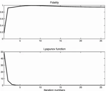
0"2e1,50.---- - -,--- - - --,--- - - ---,-- - - ---,-- - - ----,-,
Fidelity
0.6 0.4
Taking the Lyapunov function (11.4) for these dynamics we have
dV 2
<it
=
-E(1+
2E)eXI'Applying now the LaSalle invariance principle for the time periodic systems, we now that the trajectories of (111.3) converge to the largest invariant set included in the set of points whereXl
=
0. This is easy to see that this set is in fact nothing than the origin. Therefore, the error trajectories must converge to zero and we have the proof of the convergence.25 20 Lyapunov function 10 15 0.2 40
Taking e
=
1 and E=
.3, and computing the observergains as in above, we find:
Fig. 1. Average over 50 noise realizations: the first plot illustrate the evolution of the fidelity versus iteration numbers where the measurement time is taken to beT = 3 and the number of iterations 25; the second plot illustrate the evolution of the Lyapunov function (11.4) versus iteration numbers.
::
:\
0 '---""- -'--- - - -'-- - - --'-- - - --'-- - - --'--' x(2NT)=
e-2rNTx(0) 1-e- 2rNT iT+
re- 2rT ertw (t )dt 1 - e-2rT 0 1-e-2rNTr
T+
r 1 _ e-2rTJ
o
e-rtw(t)dt. The second scenario corresponds to the case where we apply only 1 back-and-forth iteration but for a gain ofNr: x=
Nr(y(t modT) - x (t ) ift E [0,T) x=
Nr(y(T- t modT) - x (t )) ift E [T,2T).The same kind of computations leads to the error:
x(2T)
=
e-2rNTx(0)+
rNe-2rNTI
TerNtw(t )dt+
rNI
Te-rNtw(t)dt. ApPENDIXThe aim of this appendix is to show that for fixed measurement time intervalT, a large number of
back-and-forth iterations with small-gain observers provides a better inversion quality than a small number of back-and-forth iterations with high-gain ones. In order to show this we consider the simple estimator allowing to low-pass filter a signal. We therefor consider the trivial system:
d
dt x
=
0, yet)=
x (t )+
wet),where wet) is a random white noise of amplitude 1. We consider two scenarios.
The first one corresponds to N back and forth iterations of an estimator with a gain r (extended as in Section III to
[0 ,2NT»:
:t x
=
r (y(t mod T) - x(t) iftE[0,T] mod 2T :t x=
r(y(T- t mod T) - x(t» iftE [T,2T] mod 2T.This leads to the error dynamics
1t
x=
-rx+
r wet modT) ift E [0,T] mod 2T1t
x=
-rx+
r weT- t modT) ift E[T,2T] mod 2T.Simple computations, based on variation of constant's for-mula, imply that the error afterN back and forth iterations
is given by 25 (III.2) 20 10 15 Iteration numbers
h
=
-4.7, l2=
-12.8, l3=
-5.88=
7.3,=
12.8,=
7.88.We consider a measurement time of T
=
3 and 25 back and forth iterations. The simulations of figure 1 illustrate the average result for 50 noise realizations where the initial state of the main system has been chosen randomly at each noise realization and the estimator has always been initialized at (-1/02) , -1/02),0). More precisely the first plot illustrates the value of Tr(Pk(0)p(
0)) indexed by k the number of iterations. Note that, here in order to get back to the density matrix formulation, we have renormalized the estimator XZ(T) and then we have computed the associated density matrix. The second plot illustrate the value of the Lyapunov function (11.4) after each iteration.Here, in order to finish this section, we provide a very rapid convergence analysis for the estimator. Getting back to the notations of the last section, one can extend the error dynamics over the time intervals [0,T] and [T,O] to a
2T-periodic system over[0,(0).Indeed, one can write the error
dynamics satisfied by
=
and=
as a unique evolution equation over [0,(0) satisfied by X
=
(Xl,X2, X3):
d
dtX
=
(X2 - e(1+
E)xI,X3 - (1+
E)XI ,-eXI)ift E [0,T] mod 2T
d
dtX
=
(-X2 - e(1+
E)XI,-X3+
(1+
E)xI,-eXI)ift E [T, 2T] mod 2T.
While in average, the both estimators achieve the same precision of e-2rNTX(0), the variance of the achieved error
is different for the two scenarios. Calling VI and V2 the obtained variances for the two scenarios respectively, we have: -2rT VI
=
:C(1 - e-2rNT)2_e _ 2 1 - e- 2r T r (1 - e- 2r N T)2 e- 2r T+ _
+
Tr2(1 _ e- 2r N T)2 --=-_ 2 1 - e- 2r T (1 - e- 2r T)2 and V2= rN(1 _ e-2rNT)e-2rNT 2+
rN2 (1 _ e-2r N T)+
Tr2N2e-2rNT.This is now trivial that for sufficiently large N the second
variance is larger than the first one as it tends to infinity when N goes to infinity.
REFERENCES
[1] A. Auroux and J. Blum. A nudging-based data assimilation method for oceanographic problems: the Back and Forth Nudging (BFN) algorithm.
Nonlin. Proc. Geophys., 15:305-319, 2008.
[2] J. Gambetta, W.A. Braff, A. Wallraff, S.M. Girvin, and R.J. Schoelkopf. Protocols for optimal readout of qubits using a continuous quantum nondemolition measurement. Phys. Rev. A, 76:012325, 2007. [3] S. Massar and S. Popescu. Optimal extraction of information from finite
quantum ensembles. Phys.Rev.Lett., 74:1259, 1995.
[4] A. Silberfarb, P.S. Jessen, and I.H. Deutsch. Quantum state reconstruc-tion via continiuous measurement. Phys. Rev. Lett., 95:030402, 2005. [5] G.A. Smith, A. Silberfarb, I.H. Deutsch, and P.S. Jessen. Efficient
quantum-state estimation by continuous weak measurement and dy-namical control. Phys. Rev. Lett., 97:180403.1-4, 2006.
![[PDF] Formation bootstrap loader in system software pdf [Eng] | Cours Bootstrap](data:image/gif;base64,R0lGODlhAQABAIAAAP///wAAACH5BAEAAAAALAAAAAABAAEAAAICRAEAOw==)