Locally Optimal Confidence Ball for a Gaussian Mixture Random Variable

HAL Id: hal-01002332

https://hal.archives-ouvertes.fr/hal-01002332

Submitted on 13 Jan 2015

HAL is a multi-disciplinary open access

archive for the deposit and dissemination of

sci-entific research documents, whether they are

pub-lished or not. The documents may come from

teaching and research institutions in France or

abroad, or from public or private research centers.

L’archive ouverte pluridisciplinaire HAL, est

destinée au dépôt et à la diffusion de documents

scientifiques de niveau recherche, publiés ou non,

émanant des établissements d’enseignement et de

recherche français ou étrangers, des laboratoires

publics ou privés.

Random Variable

Pierre Sendorek, Maurice Charbit, Karim Abed-Meraim, Sébastien Legoll

To cite this version:

Pierre Sendorek, Maurice Charbit, Karim Abed-Meraim, Sébastien Legoll. Locally Optimal

Confi-dence Ball for a Gaussian Mixture Random Variable. 4th Int. Conf. on Indoor Positioning and

Indoor Navigation(IPIN)„ Oct 2013, Belfort, France. �hal-01002332�

Locally Optimal Confidence Ball for a Gaussian

Mixture Random Variable

Pierre Sendorek, Maurice Charbit * Karim Abed-Meraim**

Sébastien Legoll*** * Télécom ParisTech, Paris, France pierre.sendorek@telecom-paristech.fr

** Polytech Orléans, Orléans, France *** Thales Avionics, Valence, France

Abstract—We address the problem of finding an estimator such as its associated confidence ball is the smallest possible in the case where the probability density function of the true position (or of the parameter to estimate) is a d-dimensional Gaussian mixture. As a solution, we propose a steepest descent algorithm which optimizes the position of the center of a ball such as its radius decreases at each step but still ensures that the ball centered on the optimized position contains the given probability. After convergence, the obtained solution is thus locally optimal. However our benchmarks suggest that the obtained solution is globally optimal.

Keywords — Confidence domain; Gaussian Mixture Model; Optimization; Monte-Carlo; Robust Estimation; Accuracy

I. INTRODUCTION

In navigation, it is often of practical interest to express the accuracy of a position estimator by the dimensions of its confidence domain [1]. One may ask which estimator achieves the optimal accuracy with respect to this criterion. In a Bayesian setting, when the probability density function (pdf) of the true position given the measurement is Gaussian, it is well known that the smallest ball containing the true position with a given probability is centered on the mean. In this case the best estimator is the mean. But the problem has less been studied when the probability density has less symmetries. However this situation naturally appears in navigation. When several sources are used to form the measurement vector, taking into account the probability of failure of each source results in obtaining a pdf of the position expressed as a Gaussian Mixture (GM) [2]. In this case it is interesting to have a position estimator such as its associated confidence ball is the smallest possible.

In this paper, we address the problem of finding the smallest confidence ball containing the position with a given probability. As a solution, we propose a steepest descent algorithm which optimizes the position of the center of a ball such as its radius decreases at each step but still ensures that the ball centered on the optimized position contains the given probability. After convergence, the obtained solution is thus locally optimal.

Our algorithm’s solution is compared to the globally optimal solution (computed thanks to an exhaustive search) in the 1-dimensional case. It is shown that the globally optimal solution empirically matches our algorithm's. Thus, when the

probability density function is only a single Gaussian, the obtained solution matches the optimal solution and is the mean.

II. POSITION OF THE PROBLEM

A. Probability of being in a ball

Suppose that the pdf of our

d

-dimensional parameter of interest, say

X

, is described by a GM. Let

N

_g be the number of gaussians composing the mixture, and for each component

j

from 1 to

N

_g, let_j be the weight the Gaussian in the mixture,



_j the mean of this Gaussian and

C

_j its covariance. The pdf of

X

thus writes

1

( )

. ( )

g N X j j j

p

x



f x







(1)

Where

f

_j

( )

x



N x

(

;



_j

,

C

_j

)

is the evaluation at

x

of the pdf of a Gaussian with a mean



_j and with a covariance

j

C

. We call

A

the probability of

X

to be outside a ball of center

c

and of radius

r

. The definition of

A

is given by

( , )

( , ))

(

( , )

P

r(

_X

)

.

x B c r

B c r

p

x d

A c

r

X

x











(2) B. The Problem

The problem is to find a center

c

such as the radius

r

is the smallest under the constraint that

X

has to be in this ball with an expected probability of

1





. This problem is equivalent to the following :

Find

c

such as

r

is the smallest possible under the constraint

A c r

( , )





.

As the reader may have noticed, we chose to deal with the complementary of the probability to be inside a ball. This is because the floating representation of a number is more precise in the neighborhood of 0 than in the neighborhood of 1 and since



is usually closer to 0 than 1 in practical applications, it will be preferable, instead of using the cumulative function, to

use the complementary cumulative function which is more precise in this context.

III. THE OPTIMIZATION ALGORITHM

A. Overview

This section details the principle of our algorithm, which is the original contribution of this work. Derivation of the equations will be explained in further sections, which will be decreasing in the abstraction level.

Our algorithm proceeds to

N

_g steepest descents, each steepest descent being initialized with

c





_j. The initialization step requires a value of

r

such as

A c r

( , )





. This value of

r

can be found either by interval halving, or by more sophisticated methods such as the secant method or Newton method, because

r

A c r

( , )

is a decreasing function (as a complementary cumulative function). When both of these values are found, the optimization step starts by finding which of the (small) variations

( , )

_{c r} of the couple

( , )

c r

do not change the probability of

X

to be outside the ball. This gives a set of possible directions

( , )

_{c r} such as

( , )

(

c

_c

,

_r

)

.

A c r



A



r







(3) Among all those possible directions for _c, we choose the one which leads to the greatest improvement in terms of radius : hence, the chosen direction is the steepest. The center

c

is optimized by being replaced by

c

'

 

c

_c and to finish the optimization step, instead of replacing

r

by

r



_r as a radius for the following step, the algorithm solves the equality

( ', )

A c r





in the variable

r

(e.g. by one of the already mentioned methods) which is preferred to avoid the cumulation of linearization errors during the successive steps of the optimization. Once this optimization step is finished, another begins. The process is repeated as long as (the step is not negligible) there is an improvement of the radius.

B. Steepest descent direction

To find the steepest descent direction, we want to find which are the (small) variations

( , )

c r such as (3) is satisfied

which implies that we want

,

)

( , )

0

(

_{c r}

.

A

c



r





A c

r



(4) And because _r and _c are supposed to be small, we replace the left term by Taylor's first order approximation

,

)

( , )

( , ).

(

(

_c

r

_r

A c r

_{c c r}

, ).

_r

A

c







 

A c r





A c r

, where



_c

A c r

( , )

is the gradient, which is the vector of partial derivatives according to the components of

c

and where

( , )

r

A c r



is the partial derivative of

A

according to

r

. Hence we get the equation

( ,

).

( , )

.

0

c

A c r

c r

A c r

r



 



(5)

or equivalently, since



_r

A c r

( , )

is negative

( , ).

/

(

, )

r

 

c

A c r

c



r

A c r

(6)

Since several directions are possible, the problem is now to find the steepest descent direction of _c. To do this, we take among all the vectors _cwhich have the same (small) norm, say

|

_c

|





, the one which minimizes _r . Finally, since Cauchy-Schwartz ensures the inequality

|

_c

A c r

( , ) | .



_c

A c r

( , ).

_c

|

_c

A c r

( , ) | .



 

 

 

(7)

As a consequence, the value of _r, which we want to be negative, is minimized when _c







.



_c

A c r

( , )/ |



_c

A c r

( , ) |

which saturates the left inequality in (7).

C. The algorithm

The value



is the size of the step which was supposed to be small during the calculations. But in practice, we take



so as to halve the dimensions of the actual radius and the

algorithm works. Also, to avoid oscillations around local optima, when a variation of the center leads to an increase of radius (whereas the linearization “predicted” a decrease), the step is halved. Halving can be repeated at most

N

_h times, after which the algorithm considers that the potential improvement is negligible. This translates into the constraint

/

r

 

r Q

, which results in choosing

.

( , )

|

( ,

)

|

r c

r

A c r

Q

A c r



 





with an initial value

Q



2

. Finally, the algorithm to find the optimal

( , )

c r

sums up to

MC

r

 

for(

j



1:

N

_g){

2

Q



j

c





find

r

such as

A c r

( , )





do{

.

( , )

|

( ,

)

|

r c

r

A c r

Q

A c r



 





.

( , )/ |

( , ) |

c

  



c

A c r



c

A c r

old old

( , )

(

c

,

r

)



c r

c

c

 

c

find

r

such as

A c r

( , )





if (

r

_old



r

) old old

(

( , )

c r



c

,

r

)

2

Q



Q

}while(

_Q



2

Nh₎ if(

r



r

_MC){ MC

,

MC

(

c

r

)



( , )

c r

}}

At the end of the algorithm,

(

c

_MC

,

r

_MC

)

will describe the locally optimal ball containing

X

with a probability

1





. D. Computation of the probability to be in a ball

The computation of the value of

A c r

( , )

implies the use of the generalized chi-square cumulative function, which can be efficiently computed e.g. using the algorithms in [3,4]. Indeed

( , )

( , )

_{j j}

( )

x B c r j

A c r



f x dx





 

(8) Where ( , ) j

( )

Pr(

)

x B c r

f

x dx







r



, for a variable



which

follows a generalized non central chi-square law with appropriate parameters [4]. In the following sections, this value will be computed from its analytical formula for every presented algorithm.

E. Derivative according to the center

The expression of the gradient



_c

A c r

( , )

has similarities with the expression of

A c r

( , )

which makes its Monte-Carlo computation comfortable. We derive the expression of the gradient by remarking that

' ( , ) (0, )

( ,

)

X

( ')

'

X

(

)

x B c r x B r

p

x dx

p

r

x

c dx

A c

 











(9)

Which allows to derive under the sign sum

(0, )

( , ).

(

).

c

A c r

c _{x B r} c

p

X

x c

c

dx





_





1 1 ' ( , )

. ( ').( '

)

. .

'

.

g N j j j j c j x T B c r

f x

x

C

d

x





  

 







F. Derivative according to the radius

The following derivations refer to a mapping of the Euclidean coordinates into the generalized

d

-dimensional polar coordinates. However, we won't need to explicit the integrals since the expression in polar coordinates will only be used to obtain the formula of the derivative according to the radius. The obtained integral has a pleasant expression to be mapped back into Euclidean coordinates, in which we will be

able to evaluate the integral numerically. Using (9) as a starting point, the substitution





x

/ |

x

|

and





|

x

|

leads to the generalized polar coordinates

1 0 ( ) (( ). ) ( , ) d . ( ) X r p r c d Ac r d          



  

where



is the Lebesgue measure on the unit sphere [5] which we won’t need to make more explicit for calculating the derivative 1 0 1 1 1 1 1 ' ( , ) ( ( ' ) ( ' | ' | | ' | ( ) ( 1) (( ) ) . ( ) ( ) ) ( ) . ( ) 1 ) ( ') '

( , )

g g d X N T d j j j j j r N T j j j j j x B c r r C c f x c x r d p r c d d r c d d d C f x d x c x c x

A c r

                                            









































IV. MONTE CARLO COMPUTATIONS

Our choice is oriented towards numerical integration since the analytical formulae of the derivatives are unknown to the authors in the general case. Among numerical methods, we chose Monte-Carlo which is known to be insensitive to the increase of dimensionality and is an efficient way to sample the integration space at points where the integrand has significant values (far from zero). Indeed, the derivatives

( , )

c

A c r



and



_r

A c r

( , )

can both be expressed, modulo the adequate choice of the functions

g

_j, as

1

( ).

( )

g d N j j j j _x

d

f x g x x



 _





where each

j

thterm of the sum can be computed thanks to Monte-Carlo with Importance Sampling. Thus the integral

( ).

( )

d j j x

f x g x dx





(10)

is numerically computed by sampling the iid variables , 1...

(

)

d

j t t N

X

_ each one according to the law

(

_j

, .

_j

)

N



m C

where

m

is a value greater than 1. Such a choice of

m

favors realizations of

X

_{j t,} outside

B c r

( , )

which is a set where the functions

g

_j are null. Thus the pdf of each random variable

X

_{j t,} is x N x( ;_j,mC_j). Monte-Carlo approximates (10) by

, , 1 , , 1 ,

(

)

(

)

(

;

,

)

1

.

(

)

(

;

,

)

d d N j j t j j t t j t j j N j j t d t d j t j j

f X

g X

N X

mC

f X

N

N X

N

mC





 





which tends to the ratio of the expectations

( )

( )

( ;

,

)

( ;

,

)

( ')

( ';

,

)

'

( ';

,

)

j j j j j j j j j j j

f x

g x

N x

mC dx

N x

mC

f x

N x

mC dx

N x

mC













which is indeed the desired value (10), when

N

_d tends to infinity. However the strength of importance sampling in this case is that only a small amount

N

_d of drawings suffices to make the algorithm work, because the possible errors in the computation of _c and



at each step are approximately corrected at the next step thanks to the computation of the new values of _c and



which only take the current value of

( , )

c r

in consideration as a starting point to the descent. V. BENCHMARKS

In a mono dimensional setting, we compare the solution obtained by our algorithm to the globally optimal solution obtained by a greedy search on the discretized space. Our algorithm is assessed on 100 Gaussian Mixtures with randomly drawn parameters :

N

_g is drawn as

G



2

where

G

follows a geometric law of mean 4 (to avoid the trivial case

N

g



1

),



j is drawn according to a centered

Gaussian with a variance of 1 and the

C

_j



K

_j

/ 3

(which are scalars in the 1D case) where

K

_j is drawn according to a chi-square law with 3 degrees of freedom. The variances are thus drawn of the same order of magnitude than the spacing between the means of the Gaussians. This is done so because the problem is easier when the variances are too small in comparison to the spacing between the means of the Gaussians. Finally the weights



_j are drawn as

1

/

g N j j i i

U

U









, where the variables

U

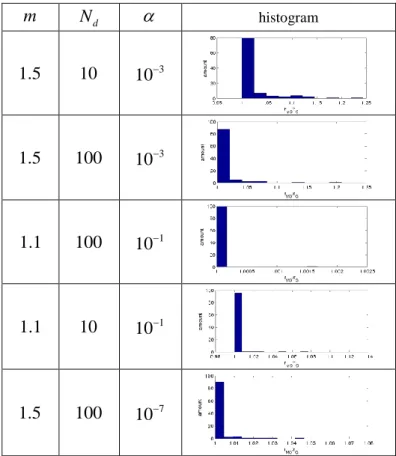
_jare iid chi-squared variables with 1 degree of freedom. For each set of these parameters, we compare the obtained radius

r

_MC with the globally optimal radius

r

_Gby computing their ratio. The evaluation is made on several sets of parameters

( ,

m N

d

, )



and for each one, a histogram of the ratio

r

MC

/

r

G is made in

figure (1). The radius obtained by our algorithm is in most of the cases the global optimum although our algorithm searches

for the best among

N

_glocal optima. The use of importance sampling enables to converge to the right result with few (100) particles even when





107.

VI. CONCLUSION

This paper has proposed a position estimator under the form of an algorithm which minimizes its associated confidence ball in the case when the position’s probability density function is expressed as a Gaussian mixture in multiple dimensions. The algorithm has been assessed in one dimension, where a comparison against greedy algorithm is possible. Numerical computations showed that the obtained confidence ball is the globally optimal one.

Figure 1. Histogram of the ratios of the obtained radius with the globally optimal radius.

REFERENCES

[1] RTCA Minimum Operational Performance Standards for Global Positioning System/Wide Area Augmentation System Airborne Equipment. 1828 L Street, NW Suite 805, Washington, D.C. 20036 USA.

[2] Pervan, Boris S., Pullen, Samuel P., Christie, Jock R., "A multiple hypothesis approach to satellite navigation integrity", Navigation, Vol. 45, No. 1, Spring 1998, pp. 61-84.

[3] Robert B Davies “Numerical inversion of a characteristic function”, Biometrika Trust, vol. 60, pp. 415-417, 1973.

[4] Robert B Davies “Algorithm AS 155: The distribution of a linear combination of 2 random variables”, Journal of the Royal Statistical Society. Series C (Applied Statistics), January 1980.

[5] Wikipedia “Spherical Measure”

http://en.wikipedia.org/wiki/Spherical_measure

m

N

_d



histogram

1.5

10

3

10



1.5

100

3

10



1.1

100

1

10



1.1

10

1

10



1.5

100

7

10

