Exact bayesian restoration in non-gaussian Markov-switching trees

HAL Id: hal-01365913

https://hal.archives-ouvertes.fr/hal-01365913

Submitted on 13 Sep 2016

HAL is a multi-disciplinary open access

archive for the deposit and dissemination of

sci-entific research documents, whether they are

pub-lished or not. The documents may come from

teaching and research institutions in France or

abroad, or from public or private research centers.

L’archive ouverte pluridisciplinaire HAL, est

destinée au dépôt et à la diffusion de documents

scientifiques de niveau recherche, publiés ou non,

émanant des établissements d’enseignement et de

recherche français ou étrangers, des laboratoires

publics ou privés.

Exact bayesian restoration in non-gaussian

Markov-switching trees

Noémie Bardel, François Desbouvries

To cite this version:

Noémie Bardel, François Desbouvries. Exact bayesian restoration in non-gaussian Markov-switching

trees. S. Co. 2009 : Complex Data Modeling and Computationally Intensive Statistical Methods for

Estimation and Prediction , Sep 2009, Milan, Italy. �hal-01365913�

E

XACT

B

AYESIAN

R

ESTORATION IN NON

-G

AUSSIAN

M

ARKOV

-S

WITCHING

T

REES

Noémie Bardel and François Desbouvries

Telecom SudParis / CITI department & CNRS UMR 5157 9, rue Charles Fourier, 91011 Evry, France

(e-mail: {noemie.bardel,francois.desbouvries}@it-sudparis.eu)

ABSTRACT. Multiresolution signal and image analysis and multiscale algorithms are of interest in many fields. In particular, efficient Bayesian restoration algorithms have been proposed for some tree-structured Markovian models. In this paper we show that Bayesian filtering and prediction can be per-formed exactly, with complexity linear in time index, in a particular class of Triplet Markov Trees.

1

INTRODUCTION

Multiresolution signal and image analysis and multiscale algorithms are of interest in many fields (Daubechies et al. (1992), Krim et al. (1999) and Starck and Bijaoui (1998)). In par-ticular, efficient restoration algorithms in statistical models defined on Hidden Markov trees (HMT) have been developed (see e.g. Chou et al. (1994), Laferté et al. (2000) or Willsky (2002)).

Let us first briefly recall the definition of a Markov Tree (MT). Let

S

be a finite set of indices and let us consider a tree with nodes indexed by

S

. Let us consider a partition

S

= {

S

1,

S

2, ...,

S

N}, where

S

nare the generations of the tree :

S

1is the root node r,

S

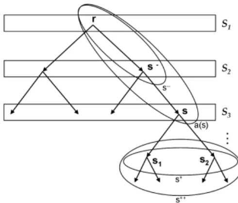
2is the

set of its children, and so on. Each node s except the root node r has exactly one parent s−, the set of the children of s is denoted by s+, the set of all descendants of s by s++and the set of all ancestors of s by s−−. We also denote by a(s) the set of all ancestors of s and s itself (i.e. a(s) = {s−−, s}).Without loss of generality we consider here the case of dyadic trees: each node s /∈ SN has exactly two children s1and s2(i.e. s+= {s1, s2})(see Fig. 1). Each node s

is associated with a random variable x(s). Also we introduce the notation x_S= {x(s), s ∈

_S

}. The tree is a Markov one if

p(x_S) = p(xr)

∏

s∈S\S1

p(xs|xs−). (1)

Let now x_S= {x(s), s ∈

_S

} and y_S= {y(s), s ∈

_S

} be two sets of variables defined on the same set

S

. Variables x(s) (resp. y(s)) are hidden (resp. observed). (x_S, y_S) is an HMT if their joint distribution satisfies:

p(x_S, y_S) = p(xr)

_∏

s∈_S\_S1

p(xs|xs−)

∏

s∈_S

p(ys|xS), (2)

i.e. x is an MT and p(y_S|x_S) = ∏s∈Sp(ys|xS). HMT have been extended to Pairwise

Markov Trees (PMT) (see Pieczynski (2002) and Desbouvries et al. (2006)) defined by: p(z_S) = p(zr)

_∏

s∈_S\_S1

in which zs= (xs, ys) and zS = (xS, yS). Any HMT is a PMT, but the converse is not true,

since in a PMT, x_S is not necessarily an MT.

We now introduce a third latent process r_Staking its values in a finite set Ω = {ω1, ..., ωt}

which can monitor for example the change of characteristics of the model. We will say that (x_S, r_S, y_S) is a Triplet Markov Tree (TMT) if it is an MT. Bayesian restoration of a hidden variable xsfrom (some of the) observed variables {ys} is in general a difficult problem. For

instance, as is well known (see Tugnait (1982)) Bayesian inference in Jump-Markov State-Space (JMSS) systems is an NP-hard problem. JMSS systems are conditionally linear and Gaussian dynamic systems, defined as:

xn+1= Fn(rn)xn+ Gn(rn)un

yn= Hn(rn)xn+ vn

in which rn is a Markov Chain, and {un}n∈{1,...,N} and {vn}n∈{1,...,N} are independent and

mutually independent zero-mean random vectors, and independent from {rn}n∈{1,...,N} and

x0. Such a model is a particular Triplet Markov Chain (xn, rn, yn), and thus a particular Triplet

Markov Tree (TMT) (xs, rs, ys) (a tree reduces to a chain if each node has exactly one child).

On the other hand, in most situations we are indeed more interested by some moment E[g(xk)|y1:n] than by pdf p(xk|y1:n) itself. In particular, the conditional expectation E[xk|y1:n]

is of particular interest since it is the solution to the Bayesian estimation problem with quadratic loss.

The aim of this paper is to show that for some particular TMT Bayesian filtering (see section 2) and prediction (see section 3) can be performed with complexity linear in time index.

2

EXACT FILTERING ON

SWITCHING-MARKOV TREES

Let x = {xs}s∈S, y = {ys}s∈Sand r = {rs}s∈Sbe sets of random variables indexed by

S

. Each

xs(resp. ys) takes its values in Rq(resp. Rm) and rstakes its values in Ω = {ω1, ..., ωt}.

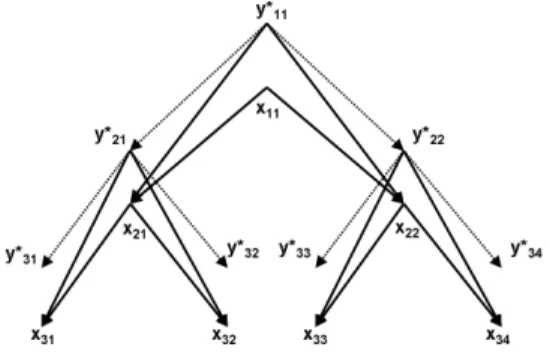
We consider the following particular TMT model(see Fig.2):

(R_S,Y_S) is a Markov Tree; (3) Xs= Fs−(R_s−,Y_s−)X_s−+U_s−; (4)

where {Us}s∈Sare independent zero-mean random vectors, such that for each s ∈

S

, Usis

in-dependent from (R_S,Y_S) and from Xr. Note that in (4) vectors Usare not necessarily Gaussian.

Figure 2. Switch-Markov Tree, with y∗= (r, y)

In this section we aim at computing E[Xs|Ya(s)= ya(s)] and Cov(Xs|Ya(s)= ya(s)) for any

s∈

_S

. Notation

For each p ∈

S

and s ∈

S

let us first set: Mp(rp, ya(s)) =

Z

Rq

xpp(xp, rp|ya(s))dxp (5)

If the covariance matrix Σpof Upexists for all p, let us set:

Vp(rp, ya(s)) =

Z

Rq

xpxpTp(xp, rp|ya(s))dxp (6)

Of course, E[Xs|Ya(s)= ya(s)] and Cov(Xs|Ya(s)= ya(s)) can be computed from Ms(rs, ya(s))

and Vs(rs, ya(s)) as:

E[Xs|Ya(s)= ya(s)] =

∑

rs

Cov(X_s|Ya(s)= ya(s)) =

∑

rs Vs(rs, ya(s)) − (

∑

rs Ms(rs, ya(s)))(

∑

rs Ms(rs, ya(s)))T.

In the following we thus focus on the computation of Ms(rs, ya(s)) and Vs(rs, ya(s)).

Proposition

Let (X_S, R_S,Y_S) satisfy (3)-(4), with given transition p(rs, ys|rs−, y_s−). Then M_s(r_s, y_a(s))

can be recursively computed with linear complexity in time by the following way:

Ms(rs, ya(s)) = 1 p(ys|ya(s−₎)

∑

r_s− p(r_s, y_s|r_s−, y_s−)F_s−(r_s−, y_s−)M_s−(r_s−, y_a(s−₎) (7) with p(y_s|ya(s−₎) = p(y_a(s)) p(y_a(s−₎) = ∑rsp(rs, ya(s)) ∑r_s−p(rs−, ya(s−)) and p(rs, ya(s)) =

∑

r_s− p(r_s−, y_a(s−₎)p(r_s, y_s|r_s−, y_s−)

Furthermore if the covariance matrix Σsof Usexists for all s ∈

S

it is possible to compute

Vs(rs, ya(s)) as: Vs(rs, ya(s)) = 1 p(ys|ya(s−₎)

∑

r_s− p(r_s, y_s|r_s−, y_s−)[F_s−(r_s−, y_s−)V_s−(r_s−, y_a(s−₎)F_s−(r_s−, y_s−)T+Σ_s−] (8) Proof

By using the Bayes formula, the fact that (X_S,Y_S, R_S) is a Markov Tree and the model (3)-(4) we have: p(x_s, r_s|ya(s)) =

∑

r_s− Z p(x_s, r_s, x_s−, r_s−|y_a(s−₎, y_s)dx_s− = 1 p(ys|ya(s−))r

∑

_s− Z p(xs, rs, xs−, rs−, ys|ya(s−₎)dx_s− = 1 p(ys|ya(s−₎)_r

∑

s− Z p(x_s−, r_s−|y_a(s−₎)p(r_s, y_s|r_s−, y_s−)p(x_s|x_s−, r_s−, y_s−)dx_s− (9)

We next multiply (9) by xs and integrate with respect to xs. Since {Us} are independent,

zero-mean and independent from (R_S,Y_S): Ms(rs, ya(s)) = 1 p(ys|ya(s−))r

∑

_s− Z p(x_s−, r_s−|y_a(s−₎)p(r_s, y_s|r_s−, y_s−)F_s−(r_s−, y_s−)x_s−dx_s− Finally:

Ms(rs, ya(s)) = 1 p(ys|ya(s−₎)_r

∑

s− p(rs, ys|rs−, ys−)Fs−(rs−, ys−) Z x_s−p(x_s−, r_s−|y_a(s−₎)dx_s− = 1 p(ys|ya(s−₎)_r

∑

s− p(rs, ys|rs−, ys−)Fs−(rs−, ys−)Ms−(rs−, ya(s−))

which brings us to the end of the proof. (8) is obtained similarly.

3

EXACT PREDICTION IN

SWITCHING-MARKOV

TREES

We consider the following particular TMT:

R_S is a Markov Tree; (10) (R_S,Y_S) is a Markov Tree; (11) Xs= Fs−(R_s−)X_s−+W_s−; (12)

where {Ws}s∈S are independent zero-mean random vectors, such that for each s ∈

S

, Ws is

independent from (R_S,Y_S) and from Xr. Note that in (12) (as in (4)) vectors Wsare not

nec-essarily Gaussian.

In this section we aim at computing E[xp|ya(s)] and Cov(xp|ya(s)) for any s ∈

S

and

p∈ s++_{. As above we focus on the computation of M}

p(rp, ya(s)) and Vp(rp, ya(s)), defined

in (5) and (6).

Proposition

Let (X_S, R_S,Y_S) satisfy (10)-(12), with given transition p(rs, ys|rs−, ys−). Then Mp(rp, ya(s))

can be recursively computed with linear complexity in time by the following scheme:

• Compute Ms(rs, ya(s)) with the algorithm presented in the last section;

• For each p ∈ s++_compute

Mp(rp, ya(s)) =

∑

r_p−

p(rp|rp−)F_p−(r_p−)M_p−(r_p−, y_a(s)). (13)

Furthermore if the covariance matrix Σsof Wsexists for all s ∈

S

it is possible to compute

Vp(rp, ya(s)) as follows:

• Compute Vs(rs, ya(s)) with the algorithm presented in the last section;

• For each p ∈ s++_compute

Vp(rp, ya(s)) =

∑

r_p−

Proof We have: p(x_p, r_p|y_a(s)) =

_∑

r_p− Z p(x_p, r_p, x_p−, r_p−|y_a(s))dx_p− =

_∑

r_p− Z p(x_p−, r_p−|y_a(s))p(x_p, r_p|x_p−, r_p−, y_a(s))dx_p− =

_∑

r_p− Z

p(x_p−, r_p−|y_a(s))p(x_p|r_p, x_p−, r_p−, y_a(s))p(r_p|x_p−, r_p−, y_a(s))dx_p− (15)

Then from (10) and (12), p(xp|rp, xp−, rp−, ya(s)) reduces to p(xp|xp−, rp−) and

p(r_p|x_p−, r_p−, y_a(s)) reduces to p(r_p|r_p−). We next multiply (15) by x_p and integrate with

respect to xpto get (13). (14) is obtained similarly.

REFERENCES

BARDEL, N., DESBOUVRIES, F. (2009): Exact bayesian prediction in non-Gaussian Markov-switching model, Proceedings of the XIIIth International Conference on Applied Stochastic Models and Data Analysis (ASMDA), June 30 - July 3, Vilnius, Lithuania.

CHOU, K.C., WILLSKY, A.S., BENVENISTE, A. (1994): Multiscale recursive estimation, data fusion, and regularization, IEEE Trans. Autom. Control, vol. 39, pp. 464-478.

DAUBECHIES, I., MALLAT, S.M., WILLSKY, A.S. (1992): Special issue on wavelet transforms and multiresolution signal analysis (Eds.), IEEE Trans. Inform. Theory, vol. 38, pp. 529-860. DESBOUVRIES, F., LECOMTE, J., PIECZYNSKI, W. (2006): Kalman Filtering in pairwise Markov

trees, Signal Processing, vol. 86, Number 5, pp. 1049-1054.

KRIM, H., WILLINGER, W., JUDITSKI, A., TSE, D. (1999): Special issue on multiscale statistical signal analysis and its applications (Eds.), IEEE Trans. Inform. Theory, vol. 45, pp. 825-1062. LAFERTE, J.M., PEREZ, P., HEITZ, F. (2000): Discrete Markov image modeling and inference on the

quadtree, IEEE Trans. Image Process., vol. 9, pp. 390-404.

PIECZYNSKI, W. (2002): Arbres de Markov Couple - Pairwise Markov Trees, C.R.A.S - Mathéma-tiques, Vol. 335, pp. 79-82.

PIECZYNSKI, W. (2008): Exact calculation of optimal filter in semi-Markov switching model, Fourth World Conference of the International Association for Statistical Computing (IASC 2008), Decem-ber 5-8, Yokohama, Japan.

STARCK, F.M.J.-L., BIJAOUI, A. (1998): Multiscale Image Processing and Data Analysis. Cambridge, U.K.: Cambridge Univ. Press.

TUGNAIT, J.K. (1982): Adaptive estimation and identification for discrete systems with Markov jump parameters, IEEE Transactions on Automatic Control, vol.25, pp. 1054-1065.

WILLSKY, A.S. (2002): Multiresolution Markov models for signal and image processing, Proc. IEEE, vol. 90, no.8, pp. 1396-1458.