HAL Id: hal-00790752
https://hal.archives-ouvertes.fr/hal-00790752
Submitted on 21 Feb 2013
HAL is a multi-disciplinary open access
archive for the deposit and dissemination of
sci-entific research documents, whether they are
pub-lished or not. The documents may come from
teaching and research institutions in France or
abroad, or from public or private research centers.
L’archive ouverte pluridisciplinaire HAL, est
destinée au dépôt et à la diffusion de documents
scientifiques de niveau recherche, publiés ou non,
émanant des établissements d’enseignement et de
recherche français ou étrangers, des laboratoires
publics ou privés.
Indexed heat curves for 3D-model retrieval
Rachid El Khoury, Jean-Philippe Vandeborre, Mohamed Daoudi
To cite this version:
Rachid El Khoury, Jean-Philippe Vandeborre, Mohamed Daoudi. Indexed heat curves for 3D-model
retrieval. 21st International Conference on Pattern Recognition (ICPR 2012), Nov 2012, Tsukuba
Science City, Japan. pp.ICPR2012. �hal-00790752�
Indexed Heat Curves for 3D-model Retrieval
Rachid El Khoury, Jean-Philippe Vandeborre and Mohamed Daoudi
Institut Mines-T´el´ecom; T´el´ecom Lille1; LIFL (UMR 8022 Lille1/CNRS), France
{elkhoury, vandeborre, daoudi}@telecom-lille1.eu
Abstract
3D-model processing plays an important role in nu-merous applications. In this paper, we present an approach for 3D-model retrieval by creating index of closed curves in<3generated from the center of a 3D-model, using a commute time mapping function. Our mapping function respects important properties in or-der to compute robust closed curves. Each curve de-scribes a small region of the 3D-model. To describe all the mesh, we compute a set of indexed closed curves. These curves lead to creates an invariant descriptor to different transformations. Then we compute the dis-tance between models by comparing the indexed curves. In order to evaluate our method, we used shapes from SHREC 2012 database. The results show the robustness of our method on various classes of 3D-models with dif-ferent positions.
1
Introduction
In recent years, a large number of 3D graphics appli-cations show their use in several domains (digital enter-tainment, computer aided design, medical applications, etc.). These applications use 3D data which grow in numbers and detail precision. The evolution of this do-main has created the need for 3D object search engines. To search a database for 3D models that are visually similar, we must create a discriminant signature. This signature encodes the shape of 3D models and should respect the invariance to rigid and non-rigid transforma-tions, the insensitivity to noise, the robustness to topol-ogy changes, and the independence on parameters. Since a few years the creation of a such signature be-came a challenge for researchers. Several 3D-model dexing approaches and shape descriptors have been in-troduced in the literature [13]. We focus here on meth-ods based on the heat diffusion and curves.
Mahmoudi and Sapiro [7] compare histogram of pair-wise using the diffusion distances between all vertices
on the mesh. Sun et al. [11] restrict their study to the temporal domain and compute their signature by ob-serving the evolution of the heat diffusion over time. Rustamov [10] creates a descriptor vector from the evaluated eigenfunctions of Laplace-Beltrami operator. Bronstein et al. [1, 2] compute the remaining heat on each vertex after a scale time t. For scale invariance, they improve the heat kernel signature to scale-invariant heat kernel signature by scaling and shifting using a log-arithmic scale-space based on Fourier transform. A few works based on curves are presented in the lit-erature and none of them is very efficient. Lmaati et al.[6] reconstruct 3D closed curves and extract feature vector as a descriptor. This method needs to align the model into canonical position before the construction of the closed curves. Tabia et al.[12] detect feature points located at the extremities of a 3D model. For each fea-ture point, they generate a collection of closed curves based on the geodesic distance. Each feature point and its collection of closed curves represent a part of the model. Finally, they use the belief functions to define the global distance between 3D-models. This method is very sensitive to topology and a small variation of the feature point leads to a large variation in curves. We propose in this paper a novel method for 3D-model retrieval based on indexed closed curves generated from an invariant mapping function defined on the mesh us-ing the commute time distance. This paper is organized as follow. In section 2 an overview of our method is given. Section 3 presents the construction and the prop-erties of our mapping function. Section 4 is about in-dexed closed curves generations and analysis. Before the conclusion in section 6, the experiments that prove the efficiency of our approach are explored in section 5.
2
Method overview
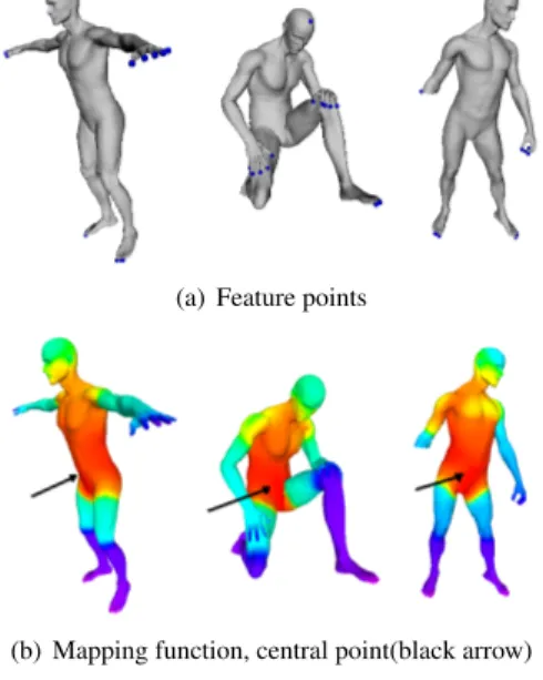
Our method starts by detecting the feature points (figure 1(a)) to define an appropriate scalar function based on the commute time distance presented in fig-ure 1(b). Then we generate and analyse indexed closed
curves raised from the center point of the 3D-model using this function (figure 1(c)). These curves are de-fined as level curves. All curves are indexed. We used Joshi et al’ s method [4] to analyse and compute the elastic metric between curves. Finally, we analyse the 3D-model by analysing the shape of their correspond-ing level curves.
(a) Feature points
(b) Mapping function, central point(black arrow)
(c) Indexed closed curves
Figure 1. The different steps of our ap-proach applied to a neutral pose model and its isometric transformation, topol-ogy change and partiality.
3
Mapping function
In order to compute robust closed curves, we need to define an appropriate invariant mapping function. We extract feature points located on the extremities of the 3D model. These feature points will be used as origins to define our mapping function.
3.1
Feature point extraction
We use the diffusion distance to extract feature points. The diffusion distance is the Euclidean distance in the spectral embedding space. It is a metric [3] de-fined using the heat kernels as
dS(t, x, y) = kK(t, x, ·) − K(t, y, ·)kL2(S) (1)
Where K(t, x, y) is the heat kernel and x, y two points defined on the mesh surface S. In a large time vari-able t, global properties are detected and the farthest two feature points are computed. In a small variable time t, from the farthest two points, we compute the lo-cal minimum diffusion distance (vertex that all its level-one neighbours have a higher value) to detect the other feature points.
3.2
Definition of our mapping function
We define our mapping function using the commute time distance. The commute-time distance is defined as: dcS(x, y)2= ∞ X i=1 1
λi(ψi(x) − ψi(y))
2 (2)
Where ψi are the eigenfunctions that correspond to λieigenvalues of Laplace-Beltrami operator satisfying ∆Sψi = λiψi. This distance takes into consideration all paths connecting a pair of vertices (x, y) on the mesh [9], a small topology change does not affect enormously the results. Based on this distance, we define our map-ping function Fmas:
Fm(v) = max(dcS(v, Vi), i = 1..nbVi)) (3) where Viis the ithfeature point, nbViis the number of feature points, dcS(v, Vi) is the commute time distance. This function computes for each vertex v the distance to the nearest feature point where the commute time distance is the highest. In figure 1(b) red to blue col-ors express the increasing values of the mapping func-tion. This function is computed using the eigenfunc-tions and eigenvalues of the Laplace-Beltrami operator. It can be seen as a global smooth scalar function and handles noisy data. For uniform scaling, we normalized the spectrum (eigenvalues) of the mesh. The mapping function is defined to be dependent only on the structure of the mesh. This makes it robust to isometric transfor-mations.
4
Extraction and analysis of closed curves
The farthest vertex of all feature points is detected by the minimum of the mapping function (figure 1(b)
Figure 2. Geodesic paths between two curves (A,B)
the black arrow points to vertex in the center of the 3D model). From this vertex, we generate indexed closed curves under a scale value of the mapping function. Each curve describes a small region. Finally the set of closed curves describes the 3D model entirely. The in-dexing of the curves saves the spatial relation between small regions. We analyse the 3D-model by analysing the shape of their corresponding level curves. To define a similarity measure between two curves, we normal-ize them, then we adopt Joshi et al.’s method [4] which analyses the shape of the curves such as one curve has to (locally) stretch, compress and bend to match the other. This is achieved by considering a large class of parametrization and by representing the curve β by the square root velocity function q(t) = √β(t)˙
k ˙βk that cap-tures its shape. Joshi et al. define a Reimanian space using elastic metric. Under this metric, they compute the length of the geodesic paths between two curves is denoted as geodesic distance between these curves. The geodesic paths can be seen as an optimal elastic defor-mation of curves such as shown on figure 2. As an ex-ample, given any two curves β1and β2, represented by its shape q1and q2. In order to handle variability such as rotation and re-parametrization the authors define or-bits as the equivalence classes of the rotation group and the re-parametrisation group that represent the q1and q2 by orbits [q1] and [q2]. To compute the geodesic paths between β1 and β2 we compute the distance between the orbits [q1] and [q2]. This task is accomplished using a path straightening approach which was introduced by Klassen and Srivastava [5].
5
Experimental results
5.1
Parameter setting of our approach
We numerically compute the eigenfunctions and the eigenvalues using the discretization proposed by Meyer et al. [8] in order to formulate the diffusion distance and the commute-time distance. We solve the general-ized eigenvalue problem using the Implicitly Restarted Arnoldi Method implemented in MATLAB. We define the basis by 50 eigenfunctions related to the 50
small-Figure 3. Precision vs Recall plot for the whole dataset
est eigenvalues. The diffusion distance is estimated in a small and in a large variable time t. For small t rang-ing in [1, 2], the diffusion is propagated significantly to detect local properties. For a large t > 15, the diffu-sion distance remains almost unchanged; so we fix it to 20. Each model is described by 50 levels of closed curves in the database. A level could contain more than one curve. The mapping function have a slight varia-tion between two similar models that leads to different levels of curves as shown at the shoulder of the par-tial 3D-model in figure1(c). To handle this variation of levels and index the right levels of the model, we de-scribe the query by 25 levels of closed curves. Each level of the query is compared to three levels of a model in the database. As an example, for a level l, this level is compared to l − 1, l, l + 1 levels with a model from the database. Then, we take the one with the smallest length of their geodesic path (the most similar). Finally, to compute the similarity measure between two mod-els, we compute the length of the geodesic path of their corresponding level curves.
5.2
Database and measures
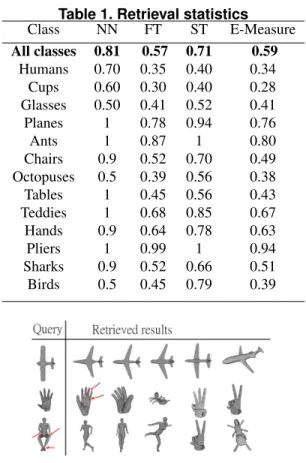
The proposed approach has been tested on a part of SHREC 2012 - Sketch-Based 3D Shape Retrieval Dataset1. The collection we used consists of 130 3D-models classified into 13 categories. Each category con-tains 10 3D-models. To evaluate our approach, we used a well-known evaluation tool: the Precision Recall plot. We plot the Precision Recall graph for the whole dataset (figure 3). Our method shows very good results due to the invariant mapping function defined on the mesh. This function describes 3D-models with different trans-formations similarly that leads to detect small region described by closed curves similarly. We also present the Nearest Neighbour (NN), First Tier (FT), Second
Table 1. Retrieval statistics Class NN FT ST E-Measure All classes 0.81 0.57 0.71 0.59 Humans 0.70 0.35 0.40 0.34 Cups 0.60 0.30 0.40 0.28 Glasses 0.50 0.41 0.52 0.41 Planes 1 0.78 0.94 0.76 Ants 1 0.87 1 0.80 Chairs 0.9 0.52 0.70 0.49 Octopuses 0.5 0.39 0.56 0.38 Tables 1 0.45 0.56 0.43 Teddies 1 0.68 0.85 0.67 Hands 0.9 0.64 0.78 0.63 Pliers 1 0.99 1 0.94 Sharks 0.9 0.52 0.66 0.51 Birds 0.5 0.45 0.79 0.39
Figure 4. Example of retrieved results.
Tier (ST) and the measure scores in table 1. The E-measure only considers the first 10 retrieved models for every query and calculates the precision and recall over those results. These scores show the excellent results of our method for some classes like Planes, Ants, Pliers, Hands, Teddies but limited results for shapes as Cups. This is due to a few number of feature points detected in objects like cups. Also, we present samples of retrieved objects in figure 4. The human model with topology changes used as a query and hands results show the ro-bustness of our method toward topology change pointed by a red arrow in figure 4.
6
Conclusion
We presented in this paper a novel approach for 3D-model retrieval. Our approach includes a method to extract stable feature points defined on the extremities. We defined an invariant mapping function to detect the center. We use the center point to generate indexed heat curves under different scale values of this function. Each curve describes a small region of the 3D-model. We index all curves in order to save the spatial
rela-tionship between small region. Finally we tested our approach and discussed the results for 3D-models re-trieval.
References
[1] A. Bronstein, M. Bronstein, L. J. Guibas, and M. Ovs-janikov. Shape google: Geometric words and expres-sions for invariant shape retrieval. ACM Transactions on Graphics, 30:1–20, 2011.
[2] M. Bronstein and I. Kokkinos. Scale-invariant heat ker-nel signatures for non-rigid shape recognition. In IEEE, Computer Vision and Pattern Recognition (CVPR), june 2010.
[3] R. R. Coifman, S. Lafon, A. B. Lee, M. Maggioni, B. Nadler, F. Warner, and S. W. Zucker. Geometric dif-fusions as a tool for harmonic analysis and structure def-inition of data: Diffusion maps. Proceedings of the Na-tional Academy of Sciences of the USA, 102(21):7426– 7431, 2005.
[4] S. H. Joshi, E. Klassen, A. Srivastava, and I. Jermyn. Removing shape-preserving transformations in square-root elastic (sre) framework for shape analysis of curves. In international conference on Energy mini-mization methods in computer vision and pattern recog-nition, EMMCVPR’07, pages 387–398, Berlin, 2007. [5] E. Klassen and A. Srivastava. Geodesics between 3d
closed curves using path-straightening. In European Conference on Computer Vision (ECCV), 2006. [6] E. A. Lmaati, A. El Oirrak, and M. N. Kaddioui. A 3d
search engine based on 3d curve analysis. Signal Image and Video Processing, 4(1):89–98, 2008.
[7] M. Mahmoudi and G. Sapiro. Three-dimensional point cloud recognition via distributions of geometric dis-tances. In IEEE, Computer Vision and Pattern Recogni-tion Workshops, pages 1 –8, june 2008.
[8] M. Meyer, M. Desbrun, P. Schr¨oder, and A. H. Barr. Discrete Differential-Geometry Operators for Triangu-lated 2-Manifolds. In VisMath ’02, Berlin, Germany, 2002.
[9] H. Qiu and E. Hancock. Clustering and embedding
using commute times. IEEE Transactions on PAMI,
29(11):1873 –1890, November 2007.
[10] R. M. Rustamov. Laplace-beltrami eigenfunctions for deformation invariant shape representation. In Proceed-ings of the fifth Eurographics symposium on Geometry processing, pages 225–233, Switzerland, 2007. [11] J. Sun, M. Ovsjanikov, and L. J. Guibas. A concise
and provably informative multi-scale signature based on heat diffusion. Comput. Graph. Forum, (5):1383–1392, 2009.
[12] H. Tabia, M. Daoudi, J. P. Vandeborre, and O. Colot. Local visual patch for 3d shape retrieval. In ACM work-shop on 3D object retrieval, pages 3–8. ACM, 2010. [13] J. W. H. Tangelder and R. C. Veltkamp. A survey of
content based 3d shape retrieval methods. In Multime-dia Tools and Applications, pages 441–471, 2008.