Science Arts & Métiers (SAM)
is an open access repository that collects the work of Arts et Métiers Institute of
Technology researchers and makes it freely available over the web where possible.
This is an author-deposited version published in: https://sam.ensam.eu Handle ID: .http://hdl.handle.net/10985/14642
To cite this version :
Hermine TERTRAIS, Ruben IBANEZ PINILLO, Anais BARASINSKI, Chady GHNATIOS, Francisco CHINESTA - On the Proper Generalized Decomposition applied to microwave processes involving multilayered components - Mathematics and Computers in Simulation - Vol. 156, p.347-363 - 2019
Any correspondence concerning this service should be sent to the repository Administrator : [email protected]
On the Proper Generalized Decomposition applied to microwave
processes involving multilayered components
H. Tertrais
a, R. Ibañez
b, A. Barasinski
a, Ch. Ghnatios
c, F. Chinesta
d,∗aGeM Institute UMR CNRS, Ecole Centrale Nantes 1 rue de la Noe, BP 92101, F-44321 Nantes cedex 3, France bESI GROUP Chair & High Performance Computing Institute ECN, 1 rue de la Noe, BP 92101, F-44321 Nantes cedex 3, France
cNotre Dame University, Louaize P.O. Box: 72, Zouk Mikael, Zouk Mosbeh, Lebanon
dESI GROUP Chair & PIMM Laboratory, ENSAM ParisTech 151 Boulevard de l’Hôpital, F-75013 Paris France
Abstract
Many electrical and structural components are constituted of a stacking of multiple thin layers with different electromagnetic, mechanical and thermal properties. When 3D descriptions become compulsory the approximation of the fields along the thickness direction could involve thousands of nodes. To circumvent the numerical difficulties that such a rich description imply, we recently propose an in-plane–out-of-plane separated representation with the aim of computing fully 3D solutions as a sequence of 2D problems defined in the plane and others (1D) in the thickness. The main contribution of the present work is the proposal of an efficient in-plane–out-of-plane separated representation of the double-curl formulation of Maxwell equations able to address thin-layer laminates while ensuring the continuity and discontinuity of the tangential and normal electric field components respectively at the plies interface.
Keywords:Maxwell equations; Multilayered components; Regularized double-curl; Separated representation; PGD
1. Introduction
Many electrical and structural components are constituted of a stacking of multiple thin layers with different electromagnetic, mechanical and thermal properties (e.g. laminated magnetic cores and circuits when looking for reducing the eddy currents or usual composite materials). In the case of composite materials for structural parts some recent studies reveal that thin-plies laminates exhibit higher strength than their counterparts making use of thicker plies [38,39,43,37]. The main characteristic of such structural systems is that the plies composing them, and even the component itself, have a characteristic dimension (the one related to the thickness) much lower that the other in-plane
∗
Corresponding author.
E-mail addresses:[email protected](H. Tertrais),[email protected](R. Iba˜nez),
characteristic lengths. The analysis of such geometrically degenerated systems does not concern solely the mechanical performances as discussed below.
In thin-ply composite laminates we can define three scales: (i) the macroscopic one that concerns the plates or shells, that is, the component scale; (ii) the mesoscopic one evidencing its intimate multi-layered structure and consequently its heterogeneity along the component thickness, with many thin-plies exhibiting different electromagnetic, mechanical and thermal properties; and finally (iii) the microscopic scale that reveals the intimate structure of each ply, in which the reinforcement, usually consisting of continuous unidirectional carbon or glass fibers impregnated by a thermoplastic or thermoset resin, with many possible microstructures.
In fact, processes involving such composites materials are based on the use of autoclaves that ensure, just after forming, the simultaneous application of pressure and temperature for consolidating the composite while reducing as much as possible its porosity. However, such process is highly demanding in energy and time, and recently many researches target the replacement of autoclaves by other technologies. Among them, microwave heating is being considered as a nice candidate for speeding-up manufacturing processes. Here, depending on the electromagnetic properties of the reinforcement two thermal sources can coexist: dielectric losses and induction, the last related to electrically conductive reinforcements (e.g. carbon fibers).
As just discussed, both the macroscopic and the mesoscopic models (the former using in general through-the-thickness homogenized properties and the last addressing explicitly the properties of each layer composing the laminate, that results at its turn from an adequate microscopic upscaling taking into account each particular fiber arrangement into the matrix) are defined in plate or shell domains characterized by having one dimension (the thickness) several orders of magnitude lower that the other representative in-plane dimensions. This fact, even if it is not a major conceptual issue, is a real handicap for simulation purposes. This situation is not new, plate and shell theories were successfully developed many years ago and they were intensively used in structural mechanics. These theories make use of some kinematic and mechanic hypotheses to reduce the 3D nature of mechanical models to 2D reduced models defined in the plate (or shell) middle surface. In the case of elastic behaviors the derivation of such reduced models is quite simple and it constitutes the foundations of classical plate and shell theories. Today, most commercial codes for structural mechanics applications propose different type of plate and shell finite elements, even in the case of multilayered composite plates or shells.
In the context of electromagnetism the situation was similar to the one encountered in structural mechanics as discussed in [36,40], where 2D cross-section, 2.5D planar solvers and 3D arbitrary-solvers were discussed. Waveguides simulators widely employed 2.5D formulations where one of the dimensions was eliminated by assuming a particular evolution of the electromagnetic field in that direction [9,32,17]. 2.5D formulations have been also extensively considered for analyzing printed circuits [42,25].
Microscopic, mesoscopic and macroscopic models have been proposed and widely considered in engineering applications, in particular in those involving laminates. Many works concerned the microscopic homogenization of electromagnetic systems, in particular composite materials [41]. At the mesoscopic scale laminates were addressed in view of defining macroscopic approaches. Three main routes were considered: (i) laminate homogenization [29,19]; (ii) monolayer and multilayer shell elements were proposed in [2,3], where the shell impedance was derived analytically by assuming a number of simplifying hypotheses and then coupled with the electromagnetic problem solution in the external domain in order to obtain the electromagnetic fields on the shell surfaces, and from them calculating all the physics inside (it is important to note that the assumed hypotheses could, in some complex circumstances, prove defective); (iii) special elements were proposed in [7] for meshing laminates when addressing explicitly the solution inside, however, for finely representing boundary layers inside the plies the computing complexity due to the required mesh resolution could become excessive.
When 3D models become compulsory the approximation of the different fields could imply thousands of nodes distributed along the thickness direction, and consequently millions of nodes to represent the fields in the part. Today, the solution of such rich 3D models remains intractable despite the impressive progresses reached in modeling, numerical analysis, discretization techniques and computer science during the last decades. The well experienced mesh-based discretization techniques fail because the excessive number of degrees of freedom involved in the fully 3D discretization where very fine meshes are required in the thickness direction (despite its reduced dimension) and many times also in the in-plane directions to avoid too distorted meshes and also because some processes (e.g. microwaves) require fine in-plane representations. We are in a real impasse. The only getaway is to explore new discretization strategies able to circumvent or at least alleviate the drawbacks related to mesh-based discretization of fully 3D
models defined in plate or shell domains. To circumvent the just discussed issues, we proposed some years ago an efficient in-plane–out-of-plane separated representation with the aim of computing fully 3D solutions as a sequence of problems defined in the plane and others (1D) in the thickness. Thus, high-resolution 3D solutions could be computed at the cost of 2D calculations.
The use of separated representations was originally proposed for defining non-incremental solvers based on the separation of space and time [24], then they were extended for addressing the solution of multidimensional models suffering the so-called curse of dimensionality [1]. The technique based on the use of separated representations was called Proper Generalized Decomposition — PGD. The interested reader can refer to the recent reviews [10–12] and the references therein.
A direct consequence was separating the physical space. Thus in plate domains an in-plane–out-of-plane decomposition was proposed for solving 3D flows occurring in RTM – Resin Transfer Molding – processes [11], then for solving elasticity problems in plates [4] and shells [5]. In those cases the 3D solution was obtained from the solution of a sequence of 2D problems (the ones involving the in-plane coordinates) and 1D problems (the ones involving the coordinate related to the plate thickness). It is important to emphasize the fact that these approaches are radically different from standard ones. We propose a 3D solver able to compute the different unknown 3D fields without the necessity of introducing any hypothesis. The most outstanding advantage is that 3D solutions can be obtained with a computational cost characteristic of standard 2D solutions.
PGD has been used in the framework of electrical engineering [35,21,22], however these works considered mainly space–time separation for performing transient simulation in a non-incremental way.
The main contribution of the present work is the proposal of an efficient in-plane–out-of-plane separated representation of the double-curl formulation of Maxwell equations able to address thin-layer laminates while ensuring the continuity and discontinuity of the tangential and normal electric field components respectively at the plies interface. Before addressing electromagnetic models within the PGD framework, we are summarizing its main ingredients.
1.1. PGD at glance
Most of the existing model reduction techniques proceed by projecting the problem solution onto a reduced basis (this constitutes the wide class of projection-based model order reduction methods). Therefore, the construction of the reduced basis usually constitutes the first step in the solution procedure, giving rise to a second important distinction when classifying Model Order Reduction – MOR – techniques: a posteriori versus a priori model order reduction. One must be careful on the suitability of a particular reduced basis when employed for representing the solution of a particular problem, particularly if it was obtained through snapshots of slightly different problems. This difficulty (at least partially) disappears if the reduced basis is constructed at the same time that the problem is solved (in other words: a priori with no need for snapshots of different problems). Thus, each problem has its associated basis in which its solution is expressed. One could consider few vectors in the basis, leading to a reduced representation, or all the terms needed for approximating the solution up to a certain accuracy level. The Proper Generalized Decomposition (PGD), which is described in general terms in what follows proceeds in this manner.
When calculating the transient solution of a generic problem, say u(x, t), we usually consider a given basis of space functions Ni(x), i = 1, . . . , Nn, the so-called shape functions within the finite element framework, being Nn
the number of nodes. They approximate the problem solution as
u(x, t) ≈
Nn
∑
i =1
ai(t )Ni(x). (1)
This implies a space–time separated representation where the time-dependent coefficients ai(t ) are unknown at each
time instant (when proceeding incrementally) and the space functions Ni(x) are given a priori, e.g., piece-wise
polynomials. POD – Proper Orthogonal Decomposition – and Reduced Basis methodologies consider a set of global, reduced basisφi(x) for approximating the solution instead of the generic, but local, finite element functions Ni(x).
The former are expected to be more adequate to approximate the problem at hand. Thus, it results
u(x, t) ≈
R
∑
i =1
where it is expected that R ≪ Nn. Again, Eq.(2)represents a space–time separated representation where the
time-dependent coefficient must be calculated at each time instant during the incremental solution procedure. Inspired from these results, one could consider the general space–time separated representation
u(x, t) ≈
N
∑
i =1
Xi(x) · Ti(t ), (3)
where now neither the time-dependent functions Ti(t ) nor the space functions Xi(x) are a priori known. Both will be
computed on the fly when solving the problem.
As soon as one postulates that the solution of a transient problem can be expressed in the separated form(3), whose approximation functions Xi(x) and Ti(t ) will be determined during the problem solution, one could make a
step forward and assume that the solution of a multidimensional problem u(x1, . . . , xd) could be found in the separated
form u(x1, x2, . . . , xd) ≈ N ∑ i =1 X1i(x1) · X2i(x1) · · · Xid(xd), (4)
and even more, expressing the 3D solution u(x, y, z) as a finite sum decomposition involving low-dimensional functions u(x, y, z) ≈ N ∑ i =1 Xi(x) · Yi(y) · Zi(z), (5) or u(x, y, z) ≈ N ∑ i =1 Xi(x, y) · Zi(z). (6)
Equivalently, the solution of a parametric problem u(x, t, p1, . . . , p℘) could be approximated as
u(x, t, p1, . . . , p℘) ≈ N ∑ i =1 Xi(x) · Ti(t ) · ℘ ∏ k=1 Pik( pk). (7)
For all the details on the separated representation constructor the interested reader can refer to [14] and the numerous references therein.
2. Electromagnetic formulation
The usual approach when solving a general electromagnetic problem with the finite element method is considering edge elements [28] with the double-curl formulation of Maxwell equations. The use of edge elements allows efficiently circumventing the main problems of FEM applied to electromagnetic models [23], in particular they produce spurious-free solutions and ensure the normal discontinuity and tangential continuity between different media, however some disadvantages have been also pointed out [26,27], concerning the ill-conditioning of discrete systems when the number of degrees of freedom – dof – increases. Some solutions were proposed for circumventing such issue, as for example the introduction of Lagrange multipliers, with the associate dof increase.
Many authors preferred the use of nodal-regularized formulations to avoid spurious solutions [20,16], while proposing ad-hoc solutions for accounting the transfer conditions at the material interfaces, as implemented in the ERMES software [31], consisting of duplicating the nodes located at the interfaces, for approximating the discontinuous field while enforcing the jump condition. Moreover, in these formulations a second regularization is required for addressing field singularities.
Because in the case of multilayered laminates the interfaces coincide with constant values of the out-of-plane coordinate (the thickness), implementing a discontinuous approximation within the in-plane–out-of-plane separated representation involved in the PGD seems quite simple. Thus, the modeling framework that we are considering consists of standard approximations (the use of advanced discretizations based on the use of edge elements into the PGD framework constitutes a work in progress) combined with a regularized formulation, with an ad-hoc treatment of interface transfer conditions.
The double-curl formulation is derived from the Maxwell’s equations in the frequency space, that in absence of current density in the laminate, reads
∇ ×( 1 µ∇ ×E
)
−ω2ϵE = 0, in Ω ⊂ R3 (8)
with the complex permittivityϵ given by ϵ = ϵr−i
σ
ω, (9)
and where µ, ϵr andσ represent the usual magnetic permeability, the electric permittivity and the conductivity
respectively.
The previous equation is complemented with adequate boundary conditions. Without loss of generality we are assuming in what follows Dirichlet boundary conditions in the whole domain boundary∂Ω
n × E = Etg, in ∂Ω (10)
where n refers to the unit outwards vector defined on the domain boundary. In the previous expressions Et g is the
prescribed electric field (assumed known) on the domain boundary, tangent to the boundary as Eq.(10)expresses. The weighted residual weak form is obtained by multiplying(8)by the test function E∗ (in fact by its conjugate,
E∗, to define properly scalar products being the electric field a complex field, i.e. E = Er+iEi), and then integrating
by parts, to obtain ∫ Ω 1 µ(∇ × E) · (∇ × E ∗ ) dx −ω2 ∫ Ω ϵE · E∗ dx− ∫ ∂Ω 1 µ(∇ × E) · (n × E ∗ ) dx = 0, (11)
for all test function E∗regular enough.
In the previous expression the boundary integral can be removed if the test function is assumed verifying n×E∗=0 on∂Ω where Dirichlet boundary conditions are enforced, i.e. n × E on ∂Ω. As previously indicated, in what follows for the sake of simplicity we are assuming Dirichlet boundary conditions on the whole domain boundary and then the weak form reduces to
∫ Ω 1 µ(∇ × E) · (∇ × E ∗ ) dx −ω2 ∫ Ω ϵE · E∗ dx = 0 (12)
However, it is well known that the weak form(12)produces spurious solutions because even if Eq.(8)ensures the verification of the Gauss equation ∇ · (ϵE) = 0, its discrete counterpart after approximating the different fields implied in the weak form(12)does not ensure the fulfillment of the Gauss equation. Thus, a regularization is compulsory for avoiding these spurious solutions. In what follows we consider the regularized form [31]
∇ ×( 1 µ∇ ×E ) −ϵ∇ ( 1 ϵϵµ∇ ·(ϵE) ) −ω2ϵE = 0, (13)
whose (regularized) weak form when Dirichlet boundary conditions apply on the wall domain boundary, reads ∫ Ω 1 µ(∇ × E) · (∇ × E ∗ ) dx −ω2 ∫ Ω ϵE · E∗ dx + ∫ Ω τ ϵϵµ(∇ · (ϵE)) (∇ · (ϵE ∗ )) dx − ∫ ∂Ω τ ϵϵµ(∇ · (ϵE) (n · (ϵE ∗ ))) dx = 0, (14) whereτ is the regularization coefficient proposed in [30] and that according to that reference is taken with a unit value everywhere except at the interfaces where it vanishes.
3. In-plane–out-of-plane separated representation
To ensure a high enough resolution of the electric field along the component thickness to represent the multilayered structure, we consider an in-plane–out-of-plane separated representation in Ω = Ωp×Ωt, with Ωp⊂ R2and Ωt ∈ R.
3.1. Separated representation The electric field is expressed as
E(x, y, z) ≈ N ∑ i =1 Pi(x, y) ◦ Ti(z) = ⎛ ⎜ ⎜ ⎜ ⎜ ⎜ ⎜ ⎜ ⎜ ⎜ ⎜ ⎝ N ∑ i =1 Pix(x, y) · Tix(z) N ∑ i =1 Piy(x, y) · Tiy(z) N ∑ i =1 Piz(x, y) · Tiz(z) ⎞ ⎟ ⎟ ⎟ ⎟ ⎟ ⎟ ⎟ ⎟ ⎟ ⎟ ⎠ , (15)
where “◦” refers to the Hadamard product. The different in-plane and out-of-plane functions, Pi and Tirespectively,
are complex and then they involve real and imaginary parts.
The previous separated representation leads to a separated representation of its derivatives according to ⎛ ⎜ ⎜ ⎜ ⎜ ⎜ ⎜ ⎝ ∂ Ex ∂x ∂ Ex ∂y ∂ Ex ∂z ∂ Ey ∂x ∂ Ey ∂y ∂ Ey ∂z ∂ Ez ∂x ∂ Ez ∂y ∂ Ee ∂z ⎞ ⎟ ⎟ ⎟ ⎟ ⎟ ⎟ ⎠ ≈ N ∑ i =1 ⎛ ⎜ ⎜ ⎜ ⎜ ⎜ ⎜ ⎜ ⎝ ∂ Px i ∂x ∂ Px i ∂y P x i ∂ Py i ∂x ∂ Py i ∂y P y i ∂ Pz i ∂x ∂ Pz i ∂y P z i ⎞ ⎟ ⎟ ⎟ ⎟ ⎟ ⎟ ⎟ ⎠ ◦ ⎛ ⎜ ⎜ ⎜ ⎜ ⎜ ⎜ ⎝ Tix Tix ∂T x i ∂z Tiy Tiy ∂T y i ∂z Tiz Tiz ∂T z i ∂z ⎞ ⎟ ⎟ ⎟ ⎟ ⎟ ⎟ ⎠ = N ∑ i =1 Pi(x, y) ◦ Ti(z), (16)
allowing the separated representation of all the differential operators appearing within the regularized weak form(14). However, the separated representation just proposed requires that all the model parameters accept a similar separated representation.
Consider the laminate composed of P layers, each one having uniform properties inside. If H is the total laminate thickness, and assuming for the sake of simplicity and without loss of generality that all the plies have the same thickness h, it results h = H
P. Now, we introduce the characteristic function of each plyχi(z), i = 1, . . . , P:
χi(z) =
{1 if (i − 1)h ≤ z< ih
0 elsewhere , (17)
that allows expressing the different properties in the separated form ⎧ ⎪ ⎪ ⎪ ⎪ ⎨ ⎪ ⎪ ⎪ ⎪ ⎩ µ(x, y, z) = P ∑ i =1 µi·χi(z) ϵ(x, y, z) = P ∑ i =1 ϵi·χi(z) , (18)
beingµiandϵithe permeability and complex permittivity (the one that involves the permittivity and conductivity) in
the i -layer.
3.2. Functional approximation
Now, before calculating the different functions involved in the approximation of the electric field, we must approximate them. Because it is assumed that the only heterogeneity applies along the thickness direction when moving from one ply to its neighbor, we can assume a standard continuous nodal approximation of fields Exand Ey
that moreover are continuous at the ply interfaces. For Ez the situation is a bit different, because it is continuous in
the plane but discontinuous across the ply interfaces, where the field jump reads
where j ≥ 1 denotes the common interface between plies j and j + 1, zj its out-of-plane coordinate, zj = j h, and
Ez(z−j) and Ez(z+j) denote the electric field at both sides of the interface, i.e. z −
j =zj −ν and z+j =zj+ν, with ν a
small enough coefficient ensuringν ≪ h. Discontinuities within the PGD framework were addressed in [18,15,8] in mechanical and thermal problems.
Here we consider continuous bilinear quadrilaterals, Q1 for approximating functions depending on the in-plane coordinates, i.e. Pix(x, y), Piy(x, y) and Piz(x, y). In what respect the functions depending on the out-of-plane coordinates we consider linear continuous 1D finite elements for approximating functions Tix(z) and Tiy(z), ensuring the continuity of Ex(x, y, z) and Ey(x, y, z), however in order to enforce the discontinuity of Ez(x, y, z) across the
ply interfaces, the nodes of the one-dimensional mesh attached to Ωz located at the ply interfaces and used for
approximating Tiz, are duplicated as proposed in [33,34,6,31]. This simple choice ensures the continuity of Ez in
the plane and its discontinuity across the ply interfaces. 4. PGD-based discretization
The separated representation construction proceeds by computing a term of the sum at each iteration. Assuming that the first n − 1 modes (terms of the finite sum) of the solution were already computed, En−1(x, y, z) with n ≥ 1,
the solution enrichment reads:
En(x, y, z) = En−1(x, y, z) + Pn(x, y) ◦ Tn(z), (20) where both vectors Pn and Tn containing functions Pn
i and T n
i (i = 1, 2, 3) depending on (x, y) and z respectively,
are unknown at the present iteration. The test function E∗reads E∗ =P∗◦Tn+Pn◦T∗.
The introduction of Eq.(20)into (14)results in a non-linear problem. We proceed by considering the simplest linearization strategy, an alternated directions fixed point algorithm, that proceeds by calculating Pn,kfrom Tn,k−1and then by updating Tn,k from the just calculated Pn,k where k refers to the step of the non-linear solver. The iteration procedure continues until convergence, that is, until reaching the fixed point ∥Pn,k◦Tn,k −Pn,k−1◦Tn,k−1∥ < ν
(ν being a small enough coefficient), that results in the searched functions Pn,k → Pn and Tn,k → Tn. Then, the
enrichment step continues by looking for the next mode Pn+1◦Tn+1. The enrichment stops when the model residual
becomes small enough.
When Tnis assumed known, we consider the test function E⋆given by P⋆◦Tn. By introducing the trial and test functions into the weak form and then integrating in Ωtbecause all the functions depending on the thickness coordinate
are known, we obtain a 2D weak formulation defined in Ωpwhose discretization (by using a standard discretization
strategy, e.g. finite elements) allows computing Pn.
Analogously, when Pn is assumed known, the test function E⋆is given by Pn ◦T⋆. By introducing the trial and test functions into the weak form and then integrating in Ωp because all the functions depending on the in-plane
coordinates (x, y) are at present known, we obtain a 1D weak formulation defined in Ωtwhose discretization (using
any technique for solving standard ODE equations) allows computing Tn.
As discussed in [4] this separated representation allows computing 3D solutions while keeping a computational complexity characteristic of 2D solution procedures. If we consider a hexahedral domain discretized using a regular structured grid with Nx, Nyand Nznodes in the x, y and z directions respectively, usual mesh-based discretization
strategies imply a challenging issue because the number of nodes involved in the model scales with Nx· Ny·Nz,
however, by using the separated representation and assuming that the solution involves N modes, one must solve about N 2D problems related to the functions involving the in-plane coordinates (x, y) and the same number of 1D problems related to the functions involving the thickness coordinate z. The computing time related to the solution of the one-dimensional problems can be neglected with respect to the one required for solving the two-dimensional ones. Thus, the resulting complexity scales as N · Nx· Ny. By comparing both complexities we can notice that as
soon as Nz ≫ N the use of separated representations leads to impressive computing time savings, making possible
the solution of models never until now solved, and even using light computing platforms.
Separated representations, at the heart of the PGD, can be considered for as discussed in the present work, transform a 3D problem into a sequence of problems of lower dimensionality. But separated representation can be also applied for computing parametric solutions where model parameters are considered as problem extra-coordinates, as widely considered in our former woks. The interested reader can refer to the review [13] and the numerous references therein. Thus, one can imagine considering the electromagnetic properties of the different layers as model parameters, and then as problem extra-coordinates, or the layers thicknesses or even the applied electromagnetic loading (electromagnetic
intensity and frequency). This kind of simulation is quite mature at present and the construction of those parametric solutions, also called computational vademecums, is nowadays a routine work.
It is important to note, that such vademecums, and as discussed in [13], allow for simulation, optimization, inverse analysis, uncertainty propagation and simulation-based control, all them under the stringent real-time constraint. 5. Numerical results
In this section we consider two laminates with different number of plies, 3 and 29 layers respectively. 5.1. 3-layer laminate
The first laminate of 0.5 m×0.5 m×3 mm is composed of three plies of similar thicknesses (1 mm each), depicted inFig. 1. The in-plane–out-of-plane representation of the electrical field components is expressed from a uniform mesh of the plane domain composed of 50 × 50 = 2500 Q1 bilinear finite elements while the thickness is equipped with 1D uniform mesh consisting of 3000 linear elements (1000 elements per layer).
The layers located at the top and bottom are characterized by the electromagnetic propertiesϵ = 10ϵ0,µ = µ0
andσ = 10−2 S/m, with ϵ0 andµ0the vacuum electrical permittivity and the magnetic permeability respectively.
The ply located at the center exhibits a larger electrical conductivity in order to attenuate the electrical field, being its associated electromagnetic properties given byϵ = ϵ0,µ = µ0andσ = 104S/m.
We considered such a laminate in order to enforce both kind of electromagnetic losses, the one related to dielectric losses here mostly occurring in the top and bottom layers, whereas in the central layer the losses are motivated by the larger electrical conductivity. The fact of placing the lowest electrical conductivity layers at top and bottom is to ensure the penetration of electromagnetic waves into the laminate to reach the central layer where they will be attenuated due to the larger electrical conductivity. By locating high conductivity layers at the top and bottom the electromagnetic waves cannot reach the central layer because they will be mostly suppressed in the neighborhood of the laminate boundaries.
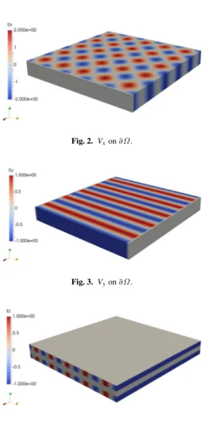
Dirichlet boundary conditions are enforced on the whole domain boundary, i.e. E × n. The tangential components of the electrical field on each face of the layers located on the domain boundary are selected from vector V
V = ⎛ ⎝ cos kx + cos ky cos ky τ cos kx ⎞ ⎠, (21)
with k = 20π, τ = 1 in the top and bottom layers and with the appropriate value in the central one for ensuring the field jump according to the Gauss law.
The components of the electrical field prescribed on the laminate boundary are depicted inFigs. 2–4for Ex, Ey
and Ezrespectively. It is important to remember that only tangential components of the electrical field are enforced
on each domain face.
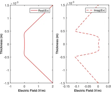
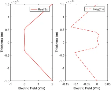
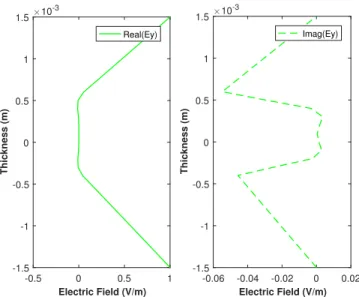
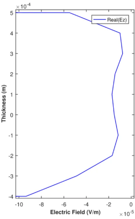
Figs. 5–7depict the evolution along the thickness of the real and imaginary parts of the three components of the electric field. In these figures the continuity of Exand Ey, and the discontinuity of Ezacross the ply interfaces can be
noticed, with a jump magnitude in agreement with the expected value.
In order to check the effects of unresolved scales related to the penetration depth, we consider a coarser mesh along the thickness composed of 30 elements (10 per layer). It can be noticed that the solution is significantly degraded with respect to solution obtained with the finer mesh as the comparison ofFigs. 5–7andFigs. 8–10reveals, in particular the out-of-plane component of the electric field Ez.
To better appreciate the unresolved boundary layer (the penetration depth beingδ = √2/ωµ0σ ≈ 0.1 mm),
Figs. 11–13depict the real part of Ez(0.25, 0.25, z) in the central layer.
It can be noticed that for resolving all the scales extremely fine meshes are required along the thickness direction, involving about thousand elements that with the thousands involved in the in-plane resolution imply meshes involving millions of elements (extremely distorted) when proceeding with standard finite elements. When using the in-plane– out-of-plane separated representation, in-plane and out-of-plane meshes become independent avoiding issues related to mesh distortion. On the other hand the problems defined in the thickness are one-dimensional and consequently their computational cost is almost negligible with respect to the solution of in-plane problems. Thus, finally the high-resolution 3D solution is obtained while keeping the computational complexity similar to the one characteristic of the solution of 2D problems (the one defined in the plane).
Fig. 1. Three-(thin)-plies laminate.
Fig. 2. Vxon∂Ω.
Fig. 3. Vyon∂Ω.
Fig. 4. Vzon∂Ω.
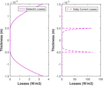
In order to emphasize the location of both kind of losses, the dielectric one and the one related to eddy currents,
Fig. 14 represents the density of both losses, where as expected, the dielectric ones locate at the external layers, whereas the one related to eddy current effects locates in the central layer and close to the interfaces where the electric field is attenuated (the penetration depth).
Fig. 5. Electrical field along the plate thickness, Ex(0.25, 0.25, z).
Fig. 6. Electrical field along the plate thickness, Ey(0.25, 0.25, z).
5.2. 29-layer laminate
The second laminate of 0.5 m×0.5 m×2.9 mm is composed of 29 plies of similar thicknesses (0.1 mm each) where two different materials are alternatively placed as illustrated inFig. 15. The in-plane–out-of-plane representation of the electrical field components is expressed from a uniform mesh of the plane domain composed of 50 × 50 = 2500 Q1 bilinear finite elements while the thickness is equipped with 1D uniform mesh consisting of 1450 linear elements (50 elements per layer).
The layers in red inFig. 15are characterized by the electromagnetic propertiesϵ = 5ϵ0,µ = µ0andσ = 0S/m,
withϵ0 andµ0 the vacuum electrical permittivity and the magnetic permeability respectively. The remaining plies
exhibit a larger electrical conductivity in order to attenuate the electrical field, being its associated electromagnetic properties given byϵ = ϵ0,µ = µ0andσ = 1S/m. The boundary conditions are the same that were enforced when
Fig. 7. Electrical field along the plate thickness, Ez(0.25, 0.25, z).
Fig. 8. Electrical field along the plate thickness, Ex(0.25, 0.25, z) when considering a coarser mesh in the thickness.
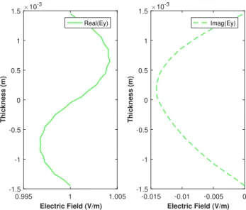
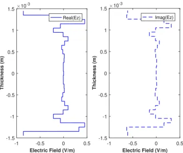
Figs. 16–18depict the evolution along the thickness of the real and imaginary parts of the three components of the electric field. In these figures the continuity of Ex and Ey, and the discontinuity of Ez across the ply interfaces
can be noticed, with a jump magnitude in agreement with the expected value. It is important to note that such a high-resolution remains out-of-reach when using standard 3D mesh-based discretization techniques, whereas the separated representation allows a very accurate solution, cheap and fast from the computational view point (the solution was obtained in 20 s using a standard laptop).
6. Discussion and conclusions
This paper proposes a new discretization technique specially appealing for addressing the propagation of electromagnetic waves in composite laminates. Because its inherent throughout-its-thickness high-resolution, direct consequence of the in-plane–out-of-plane separated representation, the reached resolution falls beyond the capabilities
Fig. 9. Electrical field along the plate thickness, Ey(0.25, 0.25, z) when considering a coarser mesh in the thickness.
Fig. 10. Electrical field along the plate thickness, Ez(0.25, 0.25, z) when considering a coarser mesh in the thickness.
of standard and well experienced mesh-based discretization techniques. By using it, micrometric resolutions can be easily reached when addressing usual composite structural parts. It allows zooming at regions exhibiting high variations of the solution, as for example the wave attenuation when reaching a conductive layer, that localizes the solution in an extremely narrow layer, whose accurate representation remains out of reach for standard discretization techniques.
The second advantage in using the proposed technique is related to the facility to enforce the jump of the normal component of the electrical field across two layers exhibiting different electromagnetic properties. For that purpose the field approximation is able to produce jumps at the laminate interfaces.
When using a high-resolution discretization based on the in-plane–out-of-plane separated representation, the double-curl electromagnetic formulation worked quite well as soon as boundary conditions were regular enough. However as soon as complex Dirichlet boundary conditions were enforced a lack of convergence was noticed and the
Fig. 11. Electrical field along the central layer thickness when considering a mesh in the thickness consisting of 30 elements.
Fig. 12. Electrical field along the central layer thickness when considering a mesh in the thickness consisting of 300 elements.
computed solutions were almost wrong. In fact the Gauss law was not fulfilled at the discrete level and for that reason a regularized formulation was considered, that allowed ensuring the solution convergence.
These three issues are subtly entangled. It is important to note that when solving the electromagnetic problem in the laminate, the z-component of the electrical field Ez is not enforced on the top and bottom surfaces. Moreover, at the
Fig. 13. Electrical field along the central layer thickness when considering a mesh in the thickness consisting of 3000 elements.
Fig. 14. Electromagnetic losses: (left) dielectric and (right) eddy current.
ply interfaces Ezjumps according to the Gauss law, and then, if the field attenuation when the wave reaches the central
(conductive) layer is not accurately described (approximated), the solution Ezbecomes wrong almost everywhere.
The consideration of perfect conductors as well as the domain decomposition for coupling standard discretization techniques and PGD separated representation, outside and inside the composite laminate respectively, are the main works in progress.
Fig. 15. 29-plies laminate. (For interpretation of the references to color in this figure legend, the reader is referred to the web version of this article.)
Fig. 16. Electrical field along the plate thickness, Ex(0.25, 0.25, z).
Fig. 18. Electrical field along the plate thickness, Ez(0.25, 0.25, z).
Acknowledgments
Authors acknowledge the contribution of some colleagues, Dr. Manuel Pineda and Dr. Enrique Nadal (from the polytechnic university of Valencia – UPV –, Spain) and Dr. Erick Abenius (from ESI Group) as well as the financial support of EU H2020 SIMUTOOL and the ESI GROUP Chairs at the Ecole Centrale of Nantes and at ENSAM ParisTech.
References
[1] A. Ammar, B. Mokdad, F. Chinesta, R. Keunings, A new family of solvers for some classes of multidimensional partial differential equations encountered in kinetic theory modeling of complex fluids, J. Non-Newton. Fluid Mech. 139 (2006) 153–176.
[2] S. Bensaid, D. Trichet, J. Fouladgar, 3D simulation of induction heating of anisotropic composite materials, IEEE Trans. Magn. 41 (5) (2005) 1568–1571.
[3] S. Bensaid, D. Trichet, J. Fouladgar, Electromagnetic and thermal behaviours of multi-layer anisotropic composite materials, IEEE Trans. Magn. 42 (4) (2006) 995–998.
[4] B. Bognet, A. Leygue, F. Chinesta, A. Poitou, F. Bordeu, Advanced simulation of models defined in plate geometries: 3D solutions with 2D computational complexity, Comput. Methods Appl. Mech. Engrg. 201 (2012) 1–12.
[5] B. Bognet, A. Leygue, F. Chinesta, Separated representations of 3D elastic solutions in shell geometries, Adv. Model. Simul. Eng. Sci. 1 (2014) 4.http://www.amses-journal.com/content/1/1/4.
[6] W.E. Boyse, D.R. Lynch, K.D. Paulsen, G.N. Minerbo, Nodal-based finite-element modeling of Maxwell’s equations, IEEE Trans. Antennas and Propagation 40 (1992) 642–651.
[7] H.K. Bui, G. Wasselynck, D. Trichet, G. Berthiau, Degenerated hexahedral whitney elements for electromagnetic fields computation in multi-layer anisotropic thin regions, IEEE Trans. Magn. 52 (3) (2016) 7208104.
[8] N. Bur, P. Joyot, Ch. Ghnatios, P. Villon, E. Cueto, F. Chinesta, Advanced computational vademecums for Automated Fibre Placement processes, Adv. Model. Simul. Eng. Sci. 3 (4) (2016),http://dx.doi.org/10.1186/s40323-016-0056-x.
[9] W.C. Chew, M.A. Nasir, A variational analysis of anisotropic, inhomogeneous dielectric waveguides, IEEE Trans. Microw. Theory Technol. 37 (4) (1989) 661–668.
[10] F. Chinesta, A. Ammar, E. Cueto, Recent advances and new challenges in the use of the Proper Generalized Decomposition for solving multidimensional models, Arch. Comput. Methods Eng. 17 (2010) 327–350.
[11] F. Chinesta, A. Ammar, A. Leygue, R. Keunings, An overview of the Proper Generalized Decomposition with applications in computational rheology, J. Non Newton. Fluid Mech. 166 (2011) 578–592.
[12] F. Chinesta, P. Ladeveze, E. Cueto, A short review in model order reduction based on Proper Generalized Decomposition, Arch. Comput. Methods Eng. 18 (2011) 395–404.
[13] F. Chinesta, A. Leygue, F. Bordeu, J.V. Aguado, E. Cueto, D. Gonzalez, I. Alfaro, A. Ammar, A. Huerta, PGD-based computational vademecum for efficient design, optimization and control, Arch. Comput. Methods Eng. 20 (2013) 31.
[14] F. Chinesta, R. Keunings, A. Leygue, The Proper Generalized Decomposition for Advanced Numerical Simulations. A primer, in: Springerbriefs, Springer, 2014.
[15] F. Chinesta, A. Leygue, B. Bognet, Ch. Ghnatios, F. Poulhaon, F. Bordeu, A. Barasinski, A. Poitou, S. Chatel, S. Maison-Le-Poec, First steps towards an advanced simulation of composites manufacturing by Automated Tape Placement, Int. J. Mater. Form. 7 (1) (2014) 81–92.
[16] M. Costabel, M. Dauge, Weighted regularization of Maxwell equations in polyhedral domains, Numer. Math. 93 (2) (2002) 239–277.
[17] G.G. Gentili, L. Accatino, A 25D FEM analysis of E-plane structures, in: 2014 International Conference on Numerical Electromagnetic Modeling and Optimization for RF, Microwave, and Terahertz Applications, NEMO, IEEE, 2014,http://dx.doi.org/10.1109/NEMO.2014. 6995689.
[18] E. Giner, B. Bognet, J.J. Rodenas, A. Leygue, J. Fuenmayor, F. Chinesta, The Proper Generalized Decomposition (PGD) as a numerical procedure to solve 3D cracked plates in linear elastic fracture mechanics, Int. J. Solids Struct. 50 (10) (2013) 1710–1720.
[19] J. Gyselinck, P. Dular, L. Krahenbuhl, R.V. Sabariego, Finite-element homogenization of laminated iron cores with inclusion of net circulating currents due to imperfect insulation, IEEE Trans. Magn. 52 (3) (2016) 7209104.
[20] C. Hazard, M. Lenoir, On the solution of the time-harmonic scattering problems for Maxwell’s equations, SIAM J. Math. Anal. 27 (1996) 1597–1630.
[21] T. Henneron, S. Clenet, Model order reduction of quasi-static problems based on POD and PGD approaches, Eur. Phys. J. - Appl. Phys. 64 (2) (2013). UNSP 24514.
[22] T. Henneron, S. Clenet, Proper Generalized Decomposition method applied to solve 3-D magnetoquasi-static field problems coupling with external electric circuits, IEEE Trans. Magn. 51 (6) (2015) 7208910.
[23] J. Jin, The Finite Element Method in Electromagnetics, second ed., John Wiley & Sons, 2002.
[24] P. Ladeveze, On a family of algorithms for structural mechanics, C. R. Math. Acad. Sci. Paris 300 (2) (1985) 41–44. (in french).
[25] E.X. Liu, X.C. Wei, E.P. Li, 2.5D methodologies for electronic package and PCB modeling: Review and latest development, in: IEEE International Symposium on Electromagnetic Compatibility, EMC, 2016.http://dx.doi.org/10.1109/ISEMC.2016.7571752.
[26] Gerrit Mur, Edge elements their advantages and their disadvantages, IEEE Trans. Magn. 30 (1994) 3552–3557.
[27] Gerrit Mur, The fallacy of edge elements, IEEE Trans. Magn. 34 (1998) 3244–3247.
[28] J.C. Nedelec, Mixed finite elements in R3, Numer. Math. 35 (1980) 315–341.
[29] I. Niyonzima, R.V. Sabariego, P. Dular, F. Henrotte, C. Geuzaine, Computational homogenization for laminated ferromagnetic cores in magnetodynamics, IEEE Trans. Magn. 49 (5) (2013) 2049–2052.
[30] R. Otin, Regularized Maxwell equations and nodal finite elements for electromagnetic field computations, J. Electromagn. 30 (1–2) (2010) 190–204.
[31] R. Otin, ERMES: A nodal-based finite element code for electromagnetic simulations in frequency domain, Comput. Phys. Comm. 184 (2013) 2588–2595.
[32] G. Pan, J. Tan, General edge element approach to lossy and dispersive structures in anisotropic media, IEEE Proc. Microw. Antennas Propag. 144 (2) (1997) 81–90.
[33] K.D. Paulsen, D.R. Lynch, J.W. Strohbehn. Three dimensional finiteboundary, and hybrid element solutions of Maxwell equations for lossy dielectric media, IEEE Trans. Microw. Theory Tech. 36 (4) (1988) 682–693.
[34] K.D. Paulsen, D.R. Lynch, J.W. Strohbehn, Numerical treatment of boundary conditions at points connecting more than two electrically distinct regions, Commun. Appl. Numer. Methods 3 (1987) 53–62.
[35] M. Pineda, F. Chinesta, J. Roger, M. Riera, J. Perez, F. Daim, Simulation of skin effect via separated representations, COMPEL - Int. J. Comput. Math. Electr. Electron. Eng. 29 (4) (2010) 919–929.
[36] J. Rautio, Some comments on EM dimensionality, IEEE M-TTS Newsl. (winter 1992) (1992) 23.
[37] H. Saito, M. Morita, K. Kawabe, M. Kanesaki, H. Takeuchi, M. Tanaka, I. Kimpara, Effect of plythickness on impact damage morphology in CFRP laminates, J. Reinf. Plast. Compos. 30 (13) (2011) 1097–1106.
[38] S. Sanchez-Saez, E. Barbero, R. Zaera, C. Navarro, Compression after impact of thin composite laminates, Compos. Sci. Technol. 65 (13) (2005) 1911–1919.
[39] S. Sihn, R.Y. Kim, K. Kawabe, S.W. Tsai, Experimental studies of thin-ply laminated composites, Compos. Sci. Technol. 67 (6) (2007) 996–1008.
[40] D.G. Swanson, W.J.R. Hoefer, Microwave Circuit Modeling Using Electromagnetic Field Simulation, Artech House, 2003.
[41] G. Wasselynck, D. Trichet, B. Ramdane, J. Fould, Interaction between electromagnetic field and CFRP materials: A new multiscale homogenization approach, IEEE Trans. Magn. 46 (8) (2010) 3277–3280.
[42] X.C. Wei, E.P. Li, E.X. Liu, R. Vahldieck, Efficient simulation of power distribution network by using integral-equation and modal-decoupling technology, IEEE Trans. Microw. Theory Tech. 56 (10) (2008) 2277–2285.
[43] T. Yokozeki, A. Kuroda, A. Yoshimura, T. Ogasawara, T. Aoki, Damage characterization in thin-ply composite laminates under out-of-plane transverse loadings, Compos. Struct. 93 (1) (2010) 49–57.