O
pen
A
rchive
T
OULOUSE
A
rchive
O
uverte (
OATAO
)
OATAO is an open access repository that collects the work of Toulouse researchers and
makes it freely available over the web where possible.
This is an author-deposited version published in :
http://oatao.univ-toulouse.fr/
Eprints ID : 18764
The contribution was presented at LICS 2016 :
http://lics.siglog.org/lics16/
To cite this version :
Cooper, Martin and Zivny, Stanislav The Power of Arc
Consistency for CSPs Defined by Partially-Ordered Forbidden Patterns.
(2016) In: 31st Annual ACM/IEEE Symposium on Logic in Computer Science
(LICS 2016), 5 July 2016 - 8 July 2016 (New York City, United States).
Any correspondence concerning this service should be sent to the repository
administrator:
[email protected]
The Power of Arc Consistency for CSPs
Defined by Partially-Ordered Forbidden Patterns
∗
Martin C. Cooper
IRIT, University of Toulouse III, FranceStanislav ˇZivn´y
Dept. of Computer Science, University of Oxford, UK [email protected]
Abstract
Characterising tractable fragments of the constraint satisfaction problem (CSP) is an important challenge in theoretical computer science and artificial intelligence. Forbidding patterns (generic sub-instances) provides a means of defining CSP fragments which are neither exclusively language-based nor exclusively structure-based. It is known that the class of binary CSP instances in which the broken-triangle pattern (BTP) does not occur, a class which in-cludes all tree-structured instances, are decided by arc consistency (AC), a ubiquitous reduction operation in constraint solvers. We provide a characterisation of simple partially-ordered forbidden patterns which have this AC-solvability property. It turns out that BTP is just one of five such AC-solvable patterns. The four other patterns allow us to exhibit new tractable classes.
Keywords arc consistency, constraint satisfaction problem, for-bidden pattern, tractability
1.
Introduction
The constraint satisfaction problem (CSP) provides a common framework for many theoretical problems in computer science as well as for many real-life applications. A CSP instance consists of a number of variables, a domain, and constraints imposed on the variables with the goal to determine whether the instance is satisfiable, that is, whether there is an assignment of domain values to all the variables in such a way that all the constraints are satisfied. The general CSP is NP-complete and thus a major research direction is to identify restrictions on the CSP that render the problem tractable, that is, solvable in polynomial time.
A substantial body of work exists from the past two decades on applications of universal algebra in the computational complexity of and the applicability of algorithmic paradigms to CSPs. More-over, a number of celebrated results have been obtained through this method; see (Barto 2014) for a recent survey. However, the alge-braic approach to CSPs is only applicable to language-based CSPs, ∗The authors were supported by EPSRC grant EP/L021226/1. Stanislav
ˇZivn´y was supported by a Royal Society University Research Fellowship.
that is, classes of CSPs defined by the set of allowed constraint re-lations but with arbitrary interactions of the constraint scopes. For instance, the well-known 2-SAT problem is a class of language-based CSPs on the Boolean domain{0, 1} with all constraint rela-tions being binary, that is, of arity at most two.
On the other side of the spectrum are structure-based CSPs, that is, classes of CSPs defined by the allowed interactions of the constraint scopes but with arbitrary constraint relations. Here the methods that have been successfully used to establish complete complexity classifications come from graph theory (Grohe 2007; Marx 2013).
The complexity of CSPs that are neither language-based nor structure-based, and thus are often called hybrid CSPs, is much less understood; see (Carbonnel and Cooper 2016) for a recent sur-vey. One approach to hybrid CSPs that has been rather successful studies the classes of CSPs defined by forbidden patterns; that is, by forbidding certain generic subinstances. The focus of this paper is on such CSPs. We remark that we deal with binary CSPs but, un-like in most papers on (the algebraic approach to) language-based CSPs, the domain is not fixed and is part of the input.
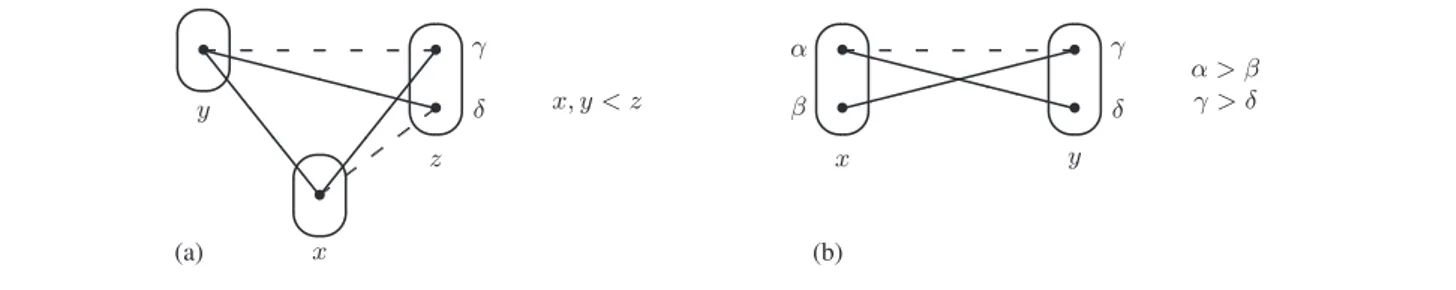
An example of a pattern is given in Figure 1(a). This is the so-called broken triangle pattern (BTP) (Cooper et al. 2010b) (a formal definition is given in Section 2). BTP is an example of a
tractable pattern, which means that any binary CSP instance in which BTP does not occur is solvable in polynomial time. The class of CSP instances defined by forbidding BTP includes, for instance, all tree-structured binary CSPs (Cooper et al. 2010b). There are several generalisations of BTP, for instance, to quanti-fied CSPs (Gao et al. 2011), to existential patterns (Cohen et al. 2015a), to patterns on more variables (Cooper et al. 2014), and other classes (Naanaa 2013; Cooper et al. 2015b).
The framework of forbidden patterns is general enough to cap-ture language-based CSPs in terms of their polymorphisms. For instance, the pattern in Figure 1(b) captures the notion of binary relations that are max-closed (Jeavons and Cooper 1995).
Surprisingly, there are essentially only two classes of algo-rithms (and their combinations) known for establishing tractability of CSPs. These are, firstly, a generalisation of Gaussian elimina-tion (Bulatov and Dalmau 2006; Dalmau 2006), whose applicabil-ity for language-based CSPs is known (Idziak et al. 2010), and, secondly, problems solvable by local consistency methods, which originated in artificial intelligence; see references in (Rossi et al. 2006). The latter can be defined in many equivalent ways includ-ing pebble games, Datalog, treewidth, and proof complexity (Feder and Vardi 1998). Intuitively, a class of CSP instances is solvable by k-consistency if unsatisfiable instances can always be refuted while only keeping partial solutions of sizek “in memory”. For instance, the 2-SAT problem is solvable by local consistency methods.
For structure-based CSPs, the power of consistency methods is well understood: a class of structures can be solved by
k-consistency if and only if the treewidth (modulo homomorphic equivalence) is at mostk (Atserias et al. 2007). Consequently, con-sistency methods solve all tractable cases of structurally-restricted bounded-arity CSPs (Grohe 2007). For language-restricted CSPs, the power of consistency methods has only recently been charac-terised (Barto and Kozik 2014; Bulatov 2009).
Contributions
Our ultimate goal is to understand the power of local consistency methods for hybrid CSPs. On this quest, we focus in this article on the power of the first level of local consistency, known as arc
consistency(AC), for classes of binary hybrid CSPs defined by forbidden (partially-ordered) patterns.
The class of CSPs defined by forbidding BTP from Figure 1(a) is in fact solvable by AC. But as it turns out, BTP is not the only pattern with this property.
As our main contribution, we give, in Theorem 12, a complete
characterisation of so-called simple partially-ordered forbidden patterns which have this AC-solvability property. Here the partial orders are on variables and domain values. It turns out that BTP is just one of five such AC-solvable patterns. The four other patterns allow us to exhibit new tractable classes, one of which in particular we expect to lead to new applications since it defines a strict generalisation of binary max-closed constraints which have already found applications in computer vision (Cooper 1999) and temporal reasoning (Dechter et al. 1991). We also provide results on the associated meta problem of deciding whether a CSP instance falls into one of these new tractable classes.
Given that AC is the first level of local consistency methods1 and is implemented in all constraint solvers, an understanding of the power of AC is paramount. We note that focusing on classes of CSPs defined by forbidden patterns is very natural as AC cannot introduce forbidden patterns. While simple patterns do not cover all partially-ordered patterns it is a natural, interesting, and broad enough concept that covers BTP and four other novel and non-trivial tractable classes. We expect our results and techniques to be used in future work on the power of AC.
Related work
Computational complexity classifications have been obtained for binary CSPs defined by forbidden negative patterns (i.e., only pair-wise incompatible assignments are specified) (Cohen et al. 2012) and for binary CSPs defined by patterns on 2 constraints (Cooper and Escamocher 2015). Moreover, (generalisations of) forbidden patterns have been studied in the context of variable and domain value elimination rules (Cohen et al. 2015a). Finally, the idea of forbidding patterns as topological minors has recently been inves-tigated (Cohen et al. 2015b).
(Kolmogorov et al. 2015; Takhanov 2015) recently considered the possible extensions of the algebraic approach from the language to the hybrid setting.
The power of the valued version of AC (Cooper et al. 2010a) has been characterised (Kolmogorov et al. 2015b). Moreover, the valued version of AC is known to solve all tractable finite-valued language-based CSPs (Thapper and ˇZivn´y).
The omitted (parts of the) proofs are given in the full version of this paper (Cooper and ˇZivn´y 2016).
1In some AI literature AC is the second level, the first being node consis-tency(Rossi et al. 2006). AC is also the first level for relational width (Bu-latov 2006).
2.
Preliminaries
2.1 CSPs and patternsA pattern can be seen as a generalisation of the concept of a binary CSP instance that leaves the consistency of some assignments to pairs of variables undefined.
Definition 1 Apattern is a four-tuplehX, D, A, cpti where:
•X is a finite set of variables; •D is a finite set of values;
•A ⊆ X × D is the set of possible variable-value assignments calledpoints; the domain ofx ∈ X is its non-empty set D(x)
of possible values:D(x) = {a ∈ D | hx, ai ∈ A};
•cpt is a partial compatibility function from the set of unordered pairs of points{{hx, ai, hy, bi} | x 6= y} to {TRUE, FALSE}. If cpt(hx, ai, hy, bi) = TRUE (resp., FALSE) we say that hx, ai
andhy, bi are compatible (resp., incompatible). For simplicity,
we writecpt(p, q) for cpt({p, q}).
We will use a simple figurative drawing for patterns. Each variable will be drawn as an oval containing dots for each of its possible points. Pairs in the domain of the functioncpt will be represented by lines between points: solid lines (called positive) for compatibility and dashed lines (called negative) for incompatibility. Example 1 The pattern in Figure 9 is called LX. It consists of three
variables, five points, six positive edges, and two negative edges.
We refine patterns to give a definition of a CSP instance. Definition 2 Abinary CSP instanceP is a pattern hX, D, A, cpti
where cpt is a total function, i.e. the domain of cpt is precisely {{hx, ai, hy, bi} | x 6= y, a ∈ D(x), b ∈ D(y)}.
•The relation Rx,y ⊆ D(x) × D(y) on hx, yi is {ha, bi |
cpt(hx, ai, hy, bi) = TRUE}.
•Apartial solution toP on Y ⊆ X is a mapping s : Y → D
where, for allx 6= y ∈ Y we have hs(x), s(y)i ∈ Rx,y. •Asolution toP is a partial solution on X.
For notational simplicity we have assumed that there is exactly
onebinary constraint between each pair of variables. In particular, this means that the absence of a constraint between variablesx, y is modelled by a complete relationRx,y= D(x) × D(y) allowing every possible pair of assignments tox and y. We say that there is a non-trivial constraint on variablesx, y if Rx,y6= D(v) × D(y). We also use the simpler notationRijforRxi,xj.
The main focus of this paper is on ordered patterns, which additionally allow for variable and value orders.
Definition 3 Anordered pattern is a six-tuplehX, D, A, cpt, <X , <Di where:
•hX, D, A, cpti is a pattern;
•<Xis a (possibly partial) strict order onX; and •<Dis a (possibly partial) strict order onD.
A patternhX, D, A, cpti can be seen as an ordered pattern with empty variable and value orders, i.e.hX, D, A, cpt, ∅, ∅i.
Throughout the paper when we say “pattern” we implicitly mean “ordered pattern” and use the word “unordered” to empha-size, if needed, that the pattern in question is not ordered.
We do not consider patterns with structure (such as equality or order) between elements in the domains of distinct variables. Definition 4 A pattern P = hX, D, A, cpt, <X, <Di is called basic if (1)D(x) and D(y) do not intersect for distinct x, y ∈ X,
and (2)<Donly contains pairs of elementsha, bi from the domain
Example 2 The pattern in Figure 1(a) is known as thebroken triangle pattern (BTP) (Cooper et al. 2010b). BTP consists of three
variables, four points, three positive edges, two negative edges,
<X={x < z, y < z}, and <D=∅. Given a basic pattern, we can
refer to a pointhx, ai in the pattern as simply a when the variable
is clear from the context or a figure. For instance, the pointhz, γi
in Figure 1(a) can be referred to asγ.
Example 3 The pattern in Figure 1(b) is the (binary)max-closed
pattern (MC). The pattern MC consists of two variables, four points, two positive edges, one negative edge, <X= ∅, and <D={β < α, δ < γ}. MC (Figure 1(b)) together with the extra
structureα > γ is an example of a pattern that is not basic. For some of the proofs we will require patterns with additional structure, namely, the ability to enforce certain points to be distinct. Definition 5 A pattern with a disequality structure is a seven-tuple hX, D, A, cpt, <X, <D, 6=Di where:
• hX, D, A, cpt, <X, <Di is a pattern; and
• 6=D⊆ D ×D is a set of pairs of domain values that are distinct.
An example of such a pattern is given in Figure 12(b). 2.2 Pattern occurrence
Some points in a pattern are indistinguishable with respect to the rest of the pattern.
Definition 6 Two pointsa, b ∈ D(x) are mergeable in a pattern hX, D, A, cpt, <X, <Di if there is no point p ∈ A for which cpt(hx, ai, p), cpt(hx, bi, p) are both defined and cpt(hx, ai, p) 6= cpt(hx, bi, p).
Definition 7 A pattern is calledunmergeable if it does not contain
any mergeable points.
Example 4 The pointsγ and δ in BTP (Figure 1(a)) are not
merge-able since they have different compatibility with, for instance, the point in variablex. The pattern LX (Figure 9) is unmergeable.
Some points in a pattern (known as dangling points) are redun-dant in arc-consistent CSP instances and hence can be removed. Definition 8 LetP = hX, D, A, cpt, <X, <Di be a pattern. A
pointp ∈ A is called dangling if it is not ordered by <Dand if there is at most one pointq ∈ A for which cpt(p, q) is defined, and
furthermore (if defined)cpt(p, q) = TRUE.
Example 5 The point β in the pattern MC (Figure 1(b)) is not
dangling since it is ordered.
In order to use (the absence of) patterns for AC-solvability we need to define what we mean when we say that a pattern occurs in a CSP instance. We define the slightly more general notion of occur-rence of a pattern in another pattern, thus extending the definitions for unordered patterns (Cooper and Escamocher 2015). Recall that a CSP instance corresponds to the special case of a pattern whose compatibility function is total. We first make the observation that dangling points in a pattern provide no useful information since we assume that all CSP instances are arc consistent, which explains why dangling points can be eliminated from patterns.
Definition 9 A pattern issimple if it is (i) basic, (ii) has no
merge-able points, and (iii) has no dangling points.
From a given pattern it is possible to create an infinite number of equivalent patterns by adding dangling points or by duplicating points. By restricting our attention to simple patterns we avoid having to consider such patterns.
Definition 10 LetP′ = hX′, D′, A′, cpt′, <X′, <D′i and P = hX, D, A, cpt, <X, <Di be two patterns. A homomorphism from P′toP is a mapping f : A′→ A which satisfies:
•Ifcpt′(p, q) is defined, then cpt(f (p), f (q)) = cpt′(p, q).
•The mappingfvar: X′→ X, given by fvar(x′) = x if ∃a′, a
such thatf (hx′, a′i) = hx, ai, is well-defined and injective.
•Ifx′<X′y′thenfvar(x′) <Xfvar(y′).
•If a′, b′ ∈ D′(x′), a′ <D′ b′, f (hx′, a′i) = hx, ai and
f (hx′, b′i) = hx, bi then a <Db.
A consistent linear extension of a patternP = hX, D, A, cpt, <X, <Di is a pattern Pt obtained from P by first identifying any number of pairs of pointsp, q which are both mergeable and incomparable (according to<D) and then extending the orders on the variables and the domain values to total orders.
Definition 11 A patternP′ = hX′, D′, A′, cpt′, <X′, <D′i oc-curs in a patternP = hX, D, A, cpt, <X, <Di if for all consistent
linear extensionsPt
ofP , there is a homomorphism from P′toPt
. We use the notation CSPSP(P ) to represent the set of binary CSP
instances in which the patternP does not occur.
This definition extends in a natural way to patterns with a disequality structure.
Remark 1 We can adda 6= b to a pattern, without changing its
semantics, whena > b or a and b are unmergeable. Furthermore,
all domain valuesa, b in an instance are distinct so there is an
implicita 6= b.
Example 6 The pattern MC (Figure 1(b)) occurs in pattern EMC
(Figure 3) but not in patterns BTP (Figure 1(a)) or BTX (Figure 7).
For a patternP , we denote by unordered(P ) the underlying unordered pattern, that is,
unordered(hX, D, A, cpt, <X, <Di) = hX, D, A, cpti. For instance, the pattern unordered(BTP) is the pattern from Fig-ure 1(a) without the structFig-urex, y < z.
The following three simple lemmas follow from the definitions. Lemma 1 IfP occurs in Q and Q occurs in R, then P occurs in R.
Lemma 2 IfP occurs in Q and P does not occur in I, then Q does
not occur inI, i.e. CSPSP(P ) ⊆ CSPSP(Q).
Lemma 3 For any patternP , unordered(P ) occurs in P . 2.3 AC solvability
Arc consistency (AC) is a fundamental concept for CSPs. Definition 12 LetI = hX, D, A, cpti be a CSP instance. A point hx, ai ∈ A is called arc consistent if, for all variables y 6= x in X
there is some pointhy, bi ∈ A compatible with hx, ai.
The CSP instancehX, D, A, cpti is called arc consistent if A 6= ∅ and every point in A is arc consistent.
Points that are not arc-consistent cannot be part of a solu-tion so can safely be removed. There are optimal O(cd2) algo-rithms for establishing arc consistency which repeatedly remove such points (Bessi`ere et al. 2005), wherec is the number of non-trivial constraints andd the maximum domain size. Algorithms es-tablishing arc consistency are implemented in all constraint solvers. AC is a decision procedure for a CSP instance if, after establish-ing arc consistency, non-empty domains for all variables guarantee the existence of a solution. (Note that a solution can then be found without backtrack by maintaining AC during search). AC is a de-cision procedure for a class of CSP instances if AC is a dede-cision procedure for every instance from the class.
✎ ✍ ☞ ✌ • ✎ ✍ ☞ ✌ • ✎ ✍ ☞ ✌ • • ❳❳❳❳❳❳❳❳ ❭ ❭ ❭ ❭ ❭✜✜ ✜✜ ✜ x y z x, y < z γ δ (a) ✎ ✍ ☞ ✌ • • ✎ ✍ ☞ ✌ • • ❳❳❳❳❳❳❳❳ ✘✘✘✘✘✘ ✘✘ x y α > β γ > δ α β γ δ (b)
Figure 1. Two AC-solvable patterns: (a) BTP (b) MC.
✎ ✍ ☞ ✌ • ✎ ✍ ☞ ✌ • ✎ ✍ ☞ ✌ • • ❳❳❳❳ ❳❳❳❳ ❭ ❭ ❭ ❭ ❭✜✜ ✜✜ ✜ x y z x, y < z γ > δ γ δ (a) ✎ ✍ ☞ ✌ • ✎ ✍ ☞ ✌ • ✎ ✍ ☞ ✌ • • ❳❳❳❳ ❳❳❳❳ ❭ ❭ ❭ ❭ ❭✜✜ ✜✜ ✜ x y z x < y < z γ δ (b)
Figure 2. Two equivalent versions of the broken triangle property: forbidding the pattern (a) BTPdoor forbidding the pattern (b) BTPvo defines the same class of instances.
Definition 13 A patternP is called AC-solvable if AC is a decision
procedure for CSPSP(P ).
The following lemma is a straightforward consequence of the definitions.
Lemma 4 A patternP is not AC-solvable if and only if there is an
instanceI ∈ CSPSP(P ) that is arc consistent and has no solution. The following lemma follows directly from Lemmas 2 and 4. Lemma 5 IfP occurs in Q and P is not AC-solvable, then Q is
not AC-solvable.
As our main result we will, in Theorem 12, characterise all simple patterns that are AC-solvable.
2.4 Pattern symmetry and equivalence
For an ordered patternP , we denote by invDom(P ), invVar(P ) the patterns obtained fromP by inversing the domain order or the variable order, respectively.
Lemma 6 IfP is not AC-solvable, then neither is invDom(P ),
invVar(P ) or invDom(invVar(P )).
Proof: The claims follow from inversing the respective orders in the instanceI of Lemma 4 proving that P is not AC-solvable.
Some patterns define the same classes of CSP instances. Definition 14 PatternsP and P′areequivalent if
CSPSP(P ) = CSPSP(P′).
Lemma 7 IfP occurs in P′andP′occurs inP , then P, P′are
equivalent.
Example 7 Let LX<be the pattern obtained from LX (Figure 9) by
adding the partial variable ordery < z. Due to the symmetry of
LX, observe that LX and LX<are equivalent.
✎ ✍ ☞ ✌ • • ✎ ✍ ☞ ✌ • ✎ ✍ ☞ ✌ • • ❳❳❳❳ ❳❳❳❳ ✘✘✘✘✘✘ ✘✘ ❭ ❭ ❭ ❭ ❭✜✜ ✜✜ ✜ x y z y < z α > β γ > δ α β γ δ ǫ
Figure 3. The ordered pattern EMC (Extended Max-Closed)
Example 8 The two patterns shown in Figure 2 are also
equiva-lent: (a) BTPdowith structurex, y < z and c < d, and (b) BTPvo
with variable orderx < y < z. We will call these the variable-ordered and domain-variable-ordered versions of BTP, respectively, when it
is necessary to make the distinction between the two. BTP (Fig-ure 1(a)) will refer to the same pattern with the only struct(Fig-ure
x, y < z which again, by symmetry, is equivalent to both BTPdo
and BTPvo.
3.
New tractable classes solved by arc consistency
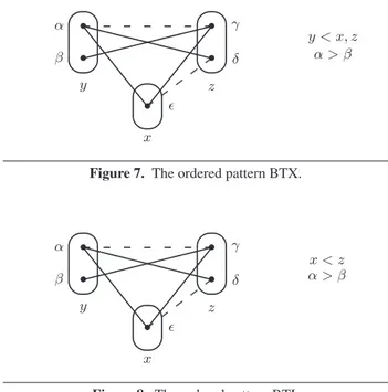
Our search for a characterisation of all simple patterns decided by arc consistency surprisingly uncovered four new tractable patterns, which we describe in this section. The first pattern we study is shown in Figure 3. It is a proper generalisation of the MC pattern (Figure 1(b)) since it has an extra variable and three extra edges. Theorem 1 AC is a decision procedure for CSPSP(EM C) whereEMC is the pattern shown in Figure 3.
Proof: Since establishing arc consistency only eliminates domain elements, and hence cannot introduce the pattern, it suffices to show that every arc-consistent instance I = hX, D, A, cpti ∈ CSPSP(EM C) has a solution. We give a constructive proof. Let
✎ ✍ ☞ ✌ • • ✎ ✍ ☞ ✌ • ✎ ✍ ☞ ✌ • • ❳❳❳❳❳❳❳❳ ✘✘✘✘✘✘ ✘✘ ❭ ❭ ❭ ❭ ❭✜✜ ✜✜ ✜ xj xmh xk xmh< xk b0> ak amh bh b0 ak aj
Figure 4. To avoid the pattern EMC, we must havebh> amh.
x1 < . . . < xnbe an ordering of X such that EMC does not occur inI. Define an assignment ha1, . . . , ani to hx1, . . . , xni recursively as follows:a1= max(D(x1)) and, for i > 1,
ai = min{aj
i| 1 ≤ j < i},
where aji = max{a ∈ D(xi)| (aj, a) ∈ Rji} (1) Fori > 1, we denote by pred(i) a value of j < i such that ai= aji. Arc consistency guarantees thata
j
i exists and hence that ai andpred(i) are well defined. We claim that ha1, . . . , ani is a solution. Suppose, for a contradiction, that(aj, ak) /∈ Rjkfor some1≤ j < k ≤ n. If there is more than one such pair (j, k), then choosek to be minimal and then for this value of k choose j to be minimal.
We prove our claim that ha1, . . . , ani is a solution to I by induction onn. The claim trivially holds for n = 1 since a1 ∈ D(x1). It remains to show that if the claim holds for instances of size less thann then it holds for instances of size n.
Letm0 = k and mr= pred(mr−1) for r ≥ 1 if mr−1> 1. Lett be such that mt= 1. By definition of pred, we have
1 = mt < mt−1 < . . . < m1 < m0= k
which implies that this series is finite and hence thatt is well-defined.
We distinguish two cases: (1)j > m1, and (2)j < m1. Since (aj, ak) /∈ Rjkand(am1, ak)∈ Rjkwe know thatj 6= m1.
Case (1)j > m1: Defineb0= aj
k. By definition ofak, we know thatak≤ ajk. Since(aj, ak) /∈ Rjkand(aj, a
j
k)∈ Rjk, we have b0= aj
k> ak.
By our choice ofj to be minimal, and since j > m1we know that(amr, ak) ∈ Rmrkforr = 1, . . . , t. Indeed, by minimality
ofk, we already had (amr, ams)∈ Rmrmsfor1≤ s ≤ r ≤ t.
Thus, sincek = m0, we have
(amr, ams)∈ Rmrms for 0≤ s ≤ r ≤ t. (2)
By arc consistency,∃b1∈ D(xm1) such that (b1, b0)∈ Rm1k.
We have (am1, aj) ∈ Rm1j by minimality of k and since
m1, j < k. Since m1 = pred(k) and hence ak = am1
k , we have(am1, ak)∈ Rm1kand(am1, b0) /∈ Rm1kby the maximal-ity ofam1
k in Equation (1). We thus have the situation illustrated in Figure 4 forh = 1. Since the pattern EMC does not occur in I, we must haveb1> am1.
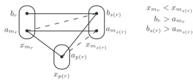
For1≤ r ≤ t, let Hrbe the following hypothesis.
Hr:∃s(r) ∈ {0, . . . , r − 1}, ∃p(r) < k, ∃br ∈ D(xmr), with
br> amr, such that we have the situation shown in Figure 5.
We have just shown thatH1holds (withs(1) = 0 and p(1) = j). We now show, for1≤ r < t, that (H1∧ . . . ∧ Hr)⇒ Hr+1.
We know that(amr+1, amr)∈ Rmr+1mrand(amr+1, br) /∈
Rmr+1mr, sincemr+1= pred(mr) and by maximality of amr=
amr+1
mr in Equation (1). Letq ∈ {0, . . . , r} be minimal such that
✎ ✍ ☞ ✌ • • ✎ ✍ ☞ ✌ • ✎ ✍ ☞ ✌ • • ❩ ❩ ❩ ❩✜✜ ✜✜ ✜ xp(r) xmr xms(r) xmr< xms(r) br> amr bs(r)> ams(r) br amr bs(r) ams(r) ap(r)
Figure 5. The situation corresponding to hypothesisHr.
✎ ✍ ☞ ✌ • • ✎ ✍ ☞ ✌ • ✎ ✍ ☞ ✌ • • ❳❳❳❳ ❳❳❳❳ ✘✘✘✘✘✘ ✘✘ ❭ ❭ ❭ ❭ ❭✜✜ ✜✜ ✜ xms(q) xmr+1 xmq xmr+1 < xmq bq> amq amr+1 br+1 bq amq bs(q)
Figure 6. To avoid the pattern EMC, we must havebr+1> amr+1.
(amr+1, bq) /∈ Rmr+1mq. We distinguish two cases: (a)q = 0,
and (b)q > 0.
Ifq = 0, then we have (amr+1, ak) ∈ Rmr+1k(from
Equa-tion (2), sincek = m0),(amr+1, b0) /∈ Rmr+1k(sinceq = 0),
(amr+1, aj)∈ Rmr+1j(by minimality ofk, since mr+1, j < k).
By arc consistency,∃br+1 ∈ D(xmr+1) such that (br+1, b0) ∈
Rmr+1k. We then have the situation illustrated in Figure 4 for
h = r + 1. As above, from the absence of pattern EMC, we can deduce thatbr+1> amr+1. We thus haveHr+1(withs(r+1) = 0
andp(r + 1) = j).
Ifq > 0, then H1 ∧ . . . ∧ Hr implies thatHq holds. By minimality of q, we know that (amr+1, bs(q)) ∈ Rmr+1ms(q)
sinces(q) < q. We know that (amr+1, amq) ∈ Rmr+1mq from
Equation (2), and that (amr+1, bq) /∈ Rmr+1mq by definition
ofq. We know that (bq, bs(q)) ∈ Rmqms(q) and(amq, bs(q)) /∈
Rmqms(q)fromHq. By arc consistency,∃br+1∈ D(xmr+1) such
that(br+1, bq)∈ Rmr+1mq. We then have the situation illustrated
in Figure 6. As above, from the absence of pattern EMC, we can deduce thatbr+1> amr+1. We thus haveHr+1(withs(r +1) = q
andp(r + 1) = s(q)).
Case (2) j < m1: Consider the subproblem I′ of I on the subset of variables{x1, x2, . . . , xm1−1} ∪ {xk}. Since xm1does
not belong to the set of variables of I′, this instance has size strictly less thann, and hence by our inductive hypothesis has a solution. The values ofaimay differ betweenI and I′. However, we can see from its definition given in Equation (1), that the value ofaidepends uniquely on the subproblem on previous variables {x1, . . . , xi−1}. Showing the dependence on the instance by a superscript, we thus haveaI′
i = aIi(i = 1, . . . , m1− 1) although aI′
k may (and, in fact, does) differ from aIk. By our inductive hypothesis,ha1, . . . , am1−1, a
I′
ki is a solution to I′. Settingb0= aI′
k, it follows that(ai, b0)∈ Rikfor1≤ i < m1. In particular, sincej < m1, we have(aj, b0) ∈ Rjk. NowaI
k ≤ aI
′
k = b0, sinceI′ is a subinstance ofI (and so, from Equation (1), aI
k is the minimum of a superset over whichaI′
k is a minimum). Thus ak= aI
✎ ✍ ☞ ✌ • • ✎ ✍ ☞ ✌ • ✎ ✍ ☞ ✌ • • ❳❳❳❳❳❳❳❳ ✘✘✘✘✘✘ ✘✘ ❭ ❭ ❭ ❭ ❭✜✜ ✜✜ ✜ x y z y < x, z α > β α β γ δ ǫ
Figure 7. The ordered pattern BTX.
✎ ✍ ☞ ✌ • • ✎ ✍ ☞ ✌ • ✎ ✍ ☞ ✌ • • ❳❳❳❳ ❳❳❳❳ ✘✘✘✘✘✘ ✘✘ ❭ ❭ ❭ ❭ ❭✜✜ ✜✜ ✜ x y z x < z α > β α β γ δ ǫ
Figure 8. The ordered pattern BTI.
By arc consistency,∃b1∈ D(xm1) such that (b1, b0)∈ Rm1k.
As in case (1), we have the situation illustrated in Figure 4 for h = 1. Since the pattern EMC does not occur in I, we must have b1> am1.
Consider the hypothesisHrstated in case (1) and illustrated in Figure 5. We have just shown thatH1 holds (withs(1) = 0 and p(1) = j). We now show, for 1 ≤ r < t, that (H1∧ . . . ∧ Hr)⇒ Hr+1.
As in case (1), we know that (amr+1, amr) ∈ Rmr+1mr
and(amr+1, br) /∈ Rmr+1mr. Letq ∈ {0, . . . , r} be minimal
such that(amr+1, bq) /∈ Rmr+1mq. We have seen above that
(amr+1, b0) ∈ Rmr+1k(sincexmr+1,xm0are assigned,
respec-tively, the valuesamr+1,b0in a solution toI
′). Therefore, we can deduce thatq > 0. Therefore H1∧ . . . ∧ Hrimplies thatHqholds. By minimality ofk, and since mq < m0 = k, we know that (amr+1, amq) ∈ Rmr+1mq. As in case (1), by minimality ofq,
we know that(amr+1, bs(q))∈ Rmr+1ms(q). By arc consistency,
∃br+1 ∈ D(xmr+1) such that (br+1, bq) ∈ Rmr+1mq. We thus
have the situation illustrated in Figure 6. Again, from the absence of pattern EMC, we can deduce thatbr+1> amr+1. We thus again
haveHr+1withs(r + 1) = q and p(r + 1) = s(q).
Thus, by induction on r, we have shown in both cases that Htholds. But recall thatmt = 1 and that a1was chosen to the maximal element ofD(x1) and hence ∄bt ∈ D(x1) such that bt> a1. This contradiction shows thatha1, . . . , ani is a solution, as claimed.
The next two patterns we study in this section, shown in Fig-ure 7 and FigFig-ure 8, are similar to EMC but the three patterns are incomparable (in the sense that none occurs in another) due to the different orders on the three variables.
Theorem 2 AC is a decision procedure for CSPSP(BT X) where
BTX is the pattern shown in Figure 7.
Theorem 3 AC is a decision procedure for CSPSP(BT I) where
BTI is the pattern shown in Figure 8.
✎ ✍ ☞ ✌ • • ✎ ✍ ☞ ✌ • ✎ ✍ ☞ ✌ • • ❳❳❳❳❳❳❳❳ ✘✘✘✘✘✘ ✘✘ ❭ ❭ ❭ ❭ ❭✜✜ ✜✜ ✜ x y z α β γ δ ǫ
Figure 9. The pattern LX.
We conclude this section with a pattern which is essentially dif-ferent from the patterns EMC, BTX, and BTI, since it includes two negative edges that meet but has no domain or variable order, and whose tractability was previously unknown (Escamocher 2014). Theorem 4 AC is a decision procedure for CSPSP(LX) where LX
is the pattern shown in Figure 9.
Proof: Since establishing arc consistency only eliminates domain elements, and hence cannot introduce the pattern, we only need to show that every arc-consistent instance I ∈ CSPSP(LX) has a solution. In fact we will show a stronger result by proving that the hypothesisHn, below, holds for alln ≥ 1.
Hn: for all arc-consistent instances I = hX, D, A, cpti ∈ CSPSP(LX) with |X| = n, ∀xi ∈ X, ∀a ∈ D(xi), I has a solutions such that s(xi) = a.
Trivially,H1holds. Suppose thatHn−1 holds wheren > 1. We will show that this impliesHn, which will complete the proof by induction.
Consider an arc-consistent instanceI = hX, D, A, cpti from CSPSP(LX) with X = {x1, . . . , xn} and let a ∈ D(xi) where 1 ≤ i ≤ n. Let In−1 denote the subproblem ofI on variables X \ {xi}. For any solution s of In−1, we denote byCV (hxi, ai, s) the set of variables inX \ {xi} on which s is compatible with the unary assignmenthxi, ai, i.e.
CV (hxi, ai, s) = {xj∈ X \ {xi} | (a, s(xj))∈ Rij} Consider two distinct solutions s, s′ toIn−1. If we have xj ∈ CV (hxi, ai, s) \ CV (hxi, ai, s′) and xk ∈ CV (hxi, ai, s′)\ CV (hxi, ai, s), then the pattern LX occurs in I under the mapping x 7→ xi,y 7→ xj,z 7→ xk,α 7→ s(xj), β 7→ s′(xj), γ 7→ s′(xk), δ 7→ s(xk), ǫ 7→ a (see Figure 9). Since LX does not occur in I, we can deduce that the sets CV (hxi, ai, s), as s varies over all solutions toIn−1, form a nested family of sets. Letsabe a solution toIn−1such thatCV (hxi, ai, sa) is maximal for inclusion.
Consider anyxj ∈ X \ {xi}. By arc consistency, ∃b ∈ D(xj) such that(a, b) ∈ Rij. By our inductive hypothesisHn−1, there is a solutions to In−1 such thats(xj) = b. Since (a, s(xj)) = (a, b) ∈ Rij, we havexj ∈ CV (hxi, ai, s). By maximality of sa, this impliesxj ∈ CV (hxi, ai, sa), i.e. (a, sa(xj))∈ Rij. Since this is true for anyxj ∈ X \ {xi}, we can deduce that sacan be extended to a solution toI (which assigns a to xi) by simply adding the assignmenthxi, ai to sa.
4.
Recognition problem for unknown orders
For an unordered pattern P of size k, checking for (the non-occurrence of)P in a CSP instance I is solvable in time O(|I|k) by simple exhaustive search. Consequently, checking for (the non-occurrence of) unordered patterns of constant size is solvable inpolynomial time. However, the situation is less obvious for ordered patterns since we have to test all possible orderings ofI.
The following result was shown in (Cooper et al. 2010b). Theorem 5 Given a binary CSP instanceI with a fixed total order
on the domain, there is a polynomial-time algorithm to find a total variable ordering such that BTP does not occur inI (or to
determine that no such ordering exists).
We show that the same result holds for the other three ordered patterns studied in this paper, namely BTI, BTX, and EMC. Theorem 6 Given a binary CSP instanceI with a fixed total order
on the domain and a patternP ∈ {BTI, BTX, EMC}, there is a
polynomial-time algorithm to find a total variable ordering such thatP does not occur in I (or to determine that no such ordering
exists).
Proof: We give a proof only for BTX as the same idea works for the other two patterns as well. Given a binary CSP instanceI with n variables x1, . . . , xn, we define an associated CSP instanceΠI that has a solution precisely when there exists a suitable variable ordering forI. To construct ΠI, letO1, . . . , Onbe variables tak-ing values in{1, . . . , n} representing positions in the ordering. We impose the ternary constraintOi> max(Oj, Ok) for all triples of variablesxi, xj, xkinI such that the BTX pattern occurs for some α, β ∈ D(xi) with α > β, ǫ ∈ D(xj), and γ, δ ∈ D(xk) when the variables are orderedxi< xj, xk. The instanceΠIhas a solution precisely if there is an ordering of the variablesx1, . . . , xnofI for which BTX does not occur. Note that if the solution obtained repre-sents a partial order (i.e. ifOiandOjare assigned the same value for somei 6= j), then it can be extended to a total order which still satisfies all the constraints by arbitrarily choosing the order of those Oi’s that are assigned the same value. This reduction is polynomial in the size ofI. We now show that all constraints in ΠIare ternary max-closed and thusΠIcan be solved in polynomial time (Jeavons and Cooper 1995). Lethp1, q1, r1i and hp2, q2, r2i satisfy any con-straint inΠI. Thenp1 > max(q1, r1) and p2 > max(q2, r2), and thus max(p1, p2) > max(max(q1, r1), max(q2, r2)) = max(max(q1, q2), max(r1, r2)). Consequently, hmax(p1, p2), max(q1, q2), max(r1, r2)i also satisfies the constraint. We can deduce that all constraints inΠIare max-closed.
Using the same technique, we can also show the following. Theorem 7 Given a binary CSP instanceI with a fixed total
vari-able order and a patternP ∈ {BTI, BTX}, there is a
polynomial-time algorithm to find a total domain ordering such thatP does not
occur inI (or determine that no such ordering exists).
It is known that determining a domain order for which MC does not occur is NP-hard (Green and Cohen 2008). Not surprisingly, for EMC when the domain order is not known, detection becomes NP-hard. For the case of BTX and BTI, if neither the domain nor variable order is known, finding orders for which the pattern does not occur is again NP-hard.
Theorem 8 For the pattern EMC, even for a fixed total variable
order of an arc-consistent binary CSP instanceI, it is NP-hard to
find a total domain ordering ofI such that the pattern does not
occur inI. For patterns BTX and BTI, it is NP-hard to find total
variable and domain orderings of an arc-consistent binary CSP instanceI such that the pattern does not occur in I.
5.
Characterisation of patterns solved by AC
5.1 Instances not solved by arc consistencyWe first give a set of instances, each of which is arc consistent and has no solution. If for any of these instancesI, we have I ∈
✗ ✖ ✔ ✕ • • • ✗ ✖ ✔ ✕ • • • ✗ ✖ ✔ ✕ • • • ✗ ✖ ✔ ✕ • • • x1 x2 x3 x4 ✭✭✭✭✭✭✭✭ ✭✭✭✭✭✭✭✭ ✭✭ ❤❤❤❤❤❤❤❤❤❤❤❤ ❤❤❤❤❤❤ ❤ ❤ ❤ ❤ ❤ ❤ ❤ ❤ ❤ ❤ ❤ ❤ ❤ ❤ ❤ ❤ ❤ ❤ ✭ ✭ ✭ ✭ ✭ ✭ ✭ ✭ ✭ ✭ ✭ ✭ ✭ ✭ ✭ ✭ ✭ ✭ ✆✆ ✆✆ ✆✆ ✆✆ ✆✆ ✆✆ ✆✆ ✆✆ ✆✆✆ ❊ ❊ ❊ ❊ ❊ ❊ ❊ ❊ ❊ ❊ ❊ ❊ ❊ ❊ ❊ ❊ ❊ ❊❊ ❊ ❊ ❊ ❊ ❊ ❊ ❊ ❊ ❊ ❊ ❊ ❊ ❊ ❊ ❊ ❊ ❊ ❊❊ ✆ ✆ ✆ ✆ ✆ ✆ ✆ ✆ ✆ ✆ ✆ ✆ ✆ ✆ ✆ ✆ ✆ ✆✆ ✁✁ ✁✁ ✁✁ ✁✁ ✁✁ ✁✁ ✓✓ ✓✓ ✓✓ ✓✓ ✓✓ ✓✓ !! !! !! !! !! !! ✟ ✟ ✟ ✟ ✟ ✟ ✟ ✟ ✟ ✟ ✟ ✟ ✚ ✚ ✚ ✚ ✚ ✚ ✚ ✚ ✚ ✚ ✚ ✚ ❆ ❆ ❆ ❆ ❆ ❆ ❆ ❆ ❆ ❆ ❆ ❆ ❙ ❙ ❙ ❙ ❙ ❙ ❙ ❙ ❙ ❙ ❙ ❙ ❅ ❅ ❅ ❅ ❅ ❅ ❅ ❅ ❅ ❅ ❅ ❅ ❍ ❍ ❍ ❍ ❍ ❍ ❍ ❍ ❍ ❍ ❍ ❍ ❩ ❩ ❩ ❩ ❩ ❩ ❩ ❩ ❩ ❩ ❩ ❩ ❍❍ ❍❍ ❍❍ ❍❍ ❍❍ ❍❍ ❩ ❩ ❩ ❩ ❩ ❩ ❩ ❩ ❩ ❩ ❩ ❩ ❅ ❅ ❅ ❅ ❅ ❅ ❅ ❅ ❅ ❅ ❅ ❅❆ ❆ ❆ ❆ ❆ ❆ ❆ ❆ ❆ ❆ ❆ ❆ ❙ ❙ ❙ ❙ ❙ ❙ ❙ ❙ ❙ ❙ ❙ ❙ ✟✟✟✟ ✟✟✟✟ ✟✟✟✟ ✚✚ ✚✚ ✚✚ ✚✚ ✚✚ ✚✚ !! !! !! !! !! !!✁✁ ✁ ✁ ✁ ✁ ✁ ✁ ✁ ✁ ✁ ✁ ✓ ✓ ✓ ✓ ✓ ✓ ✓ ✓ ✓ ✓ ✓ ✓ 1 2 3 3 2 1 1 2 3 3 2 1
Figure 10. The instanceIK4.
✓ ✒ ✏ ✑ • • ✓ ✒ ✏ ✑ • • ✓ ✒ ✏ ✑ • • ✓ ✒ ✏ ✑ • • 1 0 1 0 1 0 1 0 x1 x2 x3 x4 ❤❤❤❤❤❤❤❤❤❤❤❤ ❤❤❤ ❜ ❜ ❜❜ ❜ ❜❜ ❜ ❜ ❜❜ ❜ ❝ ❝ ❝ ❝ ❝ ❝ ❝ ❝ ❝ ❝ ❝ ❝ ❈ ❈ ❈ ❈ ❈ ❈ ❈ ❈ ❈ ❈ ❜ ❜❜ ❜ ❜ ❜❜ ❜ ❜❜ ❜ ❜ ❆ ❆ ❆ ❆ ❆ ❇ ❇ ❇ ❇ ❇ ❇ ❇❇ ✧✧ ✧✧ ✧✧ ✧✧ ✧✧ ✧✧ ✦✦✦✦ ✦✦✦✦ ✦✦✦✦ ❳❳❳❳❳❳❳❳ ❳❳ ✧✧ ✧✧ ✧✧ ✧✧ ✧✧ ✧✧ ✂✂ ✂✂ ✂✂ ✂✂ ✁✁ ✁✁ ✁ ✄✄ ✄✄ ✄✄ ✄✄ ✄✄
Figure 11. The instanceISAT K4 .
CSPSP(P ), then this constitutes a proof, by Lemma 4, that pattern P is not solved by arc consistency. For simplicity of presentation, in each of the following instances, we suppose the variable order given byxi< xjifi < j.
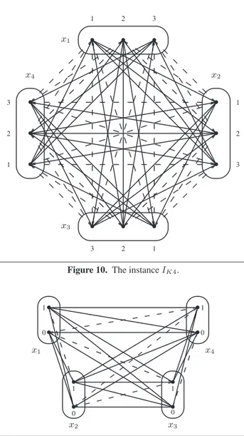
•IK4 (shown in Figure 10) is composed of four variables with domains D(xi) = {1, 2, 3} (i = 1, 2, 3, 4), and the following constraints: (xi = 1) ∨ (xj = 3) ((i, j) = (1, 2), (2, 3), (3, 4), (4, 1)) and (xi= 2)∨ (xj = 2) ((i, j) = (1, 3), (2, 4)).
•I4 is composed of four variables with domains D(x0) =
{1, 2, 3}, D(xi) = {0, 1} (i = 1, 2, 3), and the following constraints:xi∨ xj (1 ≤ i < j ≤ 3) and (x0 = i) ∨ xi (i = 1, 2, 3).
•I2∆SAT is composed of five Boolean variables and the following
constraints:x1∨x2,x3∨x4,x1∨x5,x2∨x5,x3∨x5,x4∨x5.
•I5is composed of five variables with domainsD(wi) ={0, 1}
(i = 1, 2, 3), D(xi) = {1, 2, 3}, and the constraints: wi∨ (x1 = i) (i = 1, 2, 3) and wi∨ (x2= i) (i = 1, 2, 3). In this instance the variable order isw1< w2< x1< x2< x3.
• I6SAT is composed of six Boolean variables and the following constraints:x1∨x2,x1∨x3,x1∨x4,x3∨x4,x2∨x5,x2∨x6, x5∨ x6.
• IK4SAT (shown in Figure 11) is composed of four Boolean
vari-ables and the following constraints:x1∨x2,x3∨x4andxi∨xj (for(i, j) = (1, 3), (1, 4), (2, 3), (2, 4)).
• I32COLis composed of three Boolean variables and the three inequality constraints:xi6= xj(1≤ i < j ≤ 3).
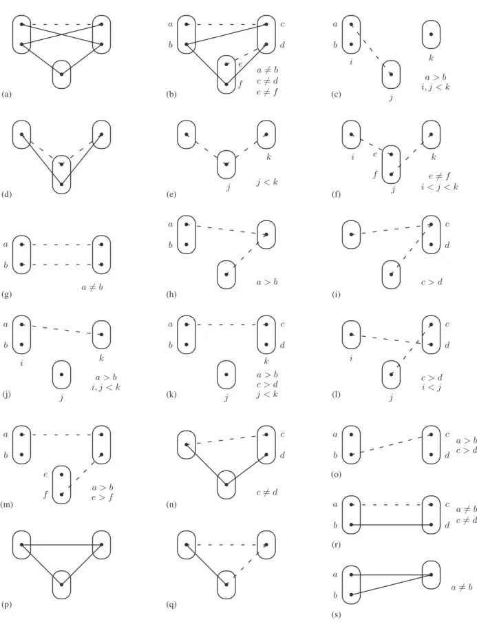
We illustrate two of these instances in Figure 10 and Figure 11. Figure 12(a) is a pattern which does not occur in the instanceIK4 (Figure 10). Similarly, Figure 12(b) is a pattern which does not occur in the instanceI4 and the pattern in Figure 12(c) does not occur in instanceISAT
2∆ . Figure 12(d), (e) and (f) are three pat-terns which do not occur in the instanceI5. The pattern (known asT 1) shown in Figure 12(d) is, in fact, a tractable pattern (Cooper and Escamocher 2015), but the fact that it does not occur inI5 (an arc-consistent instance which has no solution) shows that arc consistency is not a decision procedure for CSPSP(T 1). This in-stance was constructed using certain known properties of the pat-ternT 1 (Escamocher 2014).
It can easily be verified that the three patterns Figure 12(g), (h), (i) do not occur inISAT
6 . Similarly, the four patterns in Fig-ure 12(j),(k),(l),(m) do not occur in the instanceISAT
K4 (Figure 11). The instanceI32COL is the problem of colouring a complete graph on three vertices with only two colours. It is arc consistent but clearly has no solution. It is easy to verify that none of the six patterns in Figure 12(n),(o),(p),(q),(r),(s) occur inI32COL. Fur-thermore, trivially, no pattern on four or more variables occurs in I2COL
3 and no pattern with three or more distinct values in the same domain occurs inI2COL
3 .
By Lemma 4, we know that if a patternP does not occur in any of the instancesIK4,I4,ISAT
2∆ ,I5,I6SAT,IK4SAT,I32COL, then it is not AC-solvable. LetP be any of the patterns shown in Figure 12. By Lemma 5, any patternQ in which P occurs is not AC-solvable. By the pattern in Figure 12(g), an simple AC-solvable pattern cannot contain two negative edges between the same pair of vari-ables. Since instanceI2COL
3 contains only three variables and in-stanceI5contains no triple of variables which have a negative edge between each pair of variables, an AC-solvable pattern can con-tain at most three variables and at most two negative edges. Thus to identify simple AC-solvable patterns we only need to consider patterns on at most three variables, at most two points per variable and with none, one or two negative edges. Furthermore, in the case of two negative edges these negative edges cannot be between the same pair of variables.
5.2 Characterising AC-solvable unordered patterns
In this subsection, we consider only patternsP that have no asso-ciated structure (i.e. with<X= <D=∅). We prove the following characterisation of unstructured AC-solvable patterns.
Theorem 9 IfP is an simple unordered pattern, then P is
AC-solvable if and only ifP occurs in the pattern LX (Figure 9) or in
the pattern unordered(BTP).
Proof sketch: LetP be an simple unordered pattern. By exhaus-tive search we can deduce that either (1)P occurs in LX or un-ordered(BTP), or (2) at least one of the following patterns occurs in P : Figure 12(a), (b), (d), (n), (p), (q), (s). In case (1), by Lemma 1, Lemma 2, Lemma 3, Theorem 4 and the fact that BTP is known to be AC-solvable (Cooper et al. 2010b), it follows thatP is solvable. In case (2), since all patterns in Figure 12 are not AC-solvable, by Lemma 5,P is not AC-solvable.
5.3 Characterising AC-solvable variable-ordered patterns In this subsection we consider simple patternsP which have no domain order, but do have a partial order on the variables. We first require the following lemma.
Lemma 8 IfP<
is a pattern whose only structure is a partial order on its variables andP−= unordered(P<), then
1.P<
is simple if and only ifP−is simple.
2.P<
is AC-solvable only ifP−is AC-solvable.
Proof: The property of being simple is independent of any variable order, henceP<is simple if and only ifP−is simple. By Lemma 3, P−occurs inP<. The fact thatP<is AC-solvable only ifP−is AC-solvable then follows from Lemma 5.
Recall pattern LX< from Example 7 that is obtained from the pattern LX (Figure 9) by adding the partial variable ordery < z.
Lemma 8 allows us to give the following characterisation of variable-ordered AC-solvable patterns.
Theorem 10 IfP is an simple pattern whose only structure is a
partial order on its variables, thenP is AC-solvable if and only if P occurs in the pattern LX<, the pattern BTPvo(Figure 2) or the
pattern invVar(BTPvo).
Proof sketch: By Lemma 8 and Theorem 9, we only need to consider patterns occurring in LX or unordered(BTP) to which we add a partial order on the variables. LetP be such a pattern. By exhaustive search we can show that either (1) P occurs in LX<, BTPvoor invVar(BTPvo), or (2) at least one of the patterns in Figure 12(e), (f) occurs inP . In case (1), P is AC-solvable, sinceLX<and BTPvoare equivalent to the AC-solvable patterns LX and BTP, respectively. In case (2),P is not AC-solvable, by Lemma 5, since the patterns in Figure 12 are not AC-solvable.
5.4 Characterising AC-solvable domain-ordered patterns In this subsection we consider simple patternsP with a partial order on domains but no ordering on the variables.
Let EMC−be the no-variable-order version of the pattern EMC depicted in Figure 3.
We prove the following characterisation of domain-ordered AC-solvable patterns.
Theorem 11 IfP is an simple pattern whose only structure is a
partial order on its domains, thenP is AC-solvable if and only if P
occurs in the pattern LX (Figure 9), or the pattern EMC−, or the
pattern invDom(EMC−).
Proof sketch: As in the proofs of Theorem 9 and 10, we only need to consider patterns on at most three variables, with at most two points per variable and at most two negative edges. LetP be such a pattern. By exhaustive search, we can deduce that either (1)P occurs in LX, EMC−or invDom(EMC−), or (2) at least one of the patterns Figure 12(a), (b), (h), (i), (m), (n), (o), (p), (r), (s) (or its domain-inversed version) occurs inP .
In case (1), by Lemmas 1, 2 , 3 and Theorems 1 and 4, it follows thatP is solvable. In case (2), by Lemma 5, P is not AC-solvable, since no pattern in Figure 12 is AC-solvable.
5.5 Characterising AC-solvable ordered patterns
In this subsection we consider the most general case of simple pat-ternsP which have a partial domain order and a partial variable order. We prove the following characterisation of AC-solvable pat-terns with partial orders on domains and variables.
✎ ✍ ☞ ✌ • • ✎ ✍ ☞ ✌ • ✎ ✍ ☞ ✌ • • ❳❳❳❳ ❳❳❳❳ ✘✘✘✘✘✘ ✘✘ ❩ ❩ ❩ ❩✚✚ ✚✚ (a) ✎ ✍ ☞ ✌ • • ✎ ✍ ☞ ✌ • • ✎ ✍ ☞ ✌ • • ✘✘✘✘✘✘ ✘✘ !! !! ❅ ❅ ❅ ❅ a b c d e f a 6= b c 6= d e 6= f (b) ✎ ✍ ☞ ✌ • • ✎ ✍ ☞ ✌ • ✎ ✍ ☞ ✌ • a b i k j a > b i, j < k (c) ✎ ✍ ☞ ✌ • ✎ ✍ ☞ ✌ • • ✎ ✍ ☞ ✌ • ❭ ❭ ❭ ❭ ❭✜✜ ✜✜ ✜ (d) ✎ ✍ ☞ ✌ • ✎ ✍ ☞ ✌ • ✎ ✍ ☞ ✌ • j k j < k (e) ✎ ✍ ☞ ✌ • ✎ ✍ ☞ ✌ • • ✎ ✍ ☞ ✌ • i j k e f e 6= f i < j < k (f) ✎ ✍ ☞ ✌ • • ✎ ✍ ☞ ✌ • • a b a 6= b (g) ✎ ✍ ☞ ✌ • • ✎ ✍ ☞ ✌ • ✎ ✍ ☞ ✌ • a b a > b (h) ✎ ✍ ☞ ✌ • ✎ ✍ ☞ ✌ • ✎ ✍ ☞ ✌ • • c d c > d (i) ✎ ✍ ☞ ✌ • • ✎ ✍ ☞ ✌ • ✎ ✍ ☞ ✌ • a b i j k a > b i, j < k (j) ✎ ✍ ☞ ✌ • • ✎ ✍ ☞ ✌ • ✎ ✍ ☞ ✌ • • a b c d k j a > b c > d j < k (k) ✎ ✍ ☞ ✌ • ✎ ✍ ☞ ✌ • ✎ ✍ ☞ ✌ • • c d i j c > d i < j (l) ✎ ✍ ☞ ✌ • • ✎ ✍ ☞ ✌ • • ✎ ✍ ☞ ✌ • • a b e f a > be > f (m) ✎ ✍ ☞ ✌ • ✎ ✍ ☞ ✌ • ✎ ✍ ☞ ✌ • • ❅ ❅ ❅ ❅ ✚✚ ✚✚ c d c 6= d (n) ✎ ✍ ☞ ✌ • • ✎ ✍ ☞ ✌ • • a b c d a > b c > d (o) ✎ ✍ ☞ ✌ • ✎ ✍ ☞ ✌ • ✎ ✍ ☞ ✌ • ❅ ❅ ❅ ❅ !! !! (p) ✎ ✍ ☞ ✌ • ✎ ✍ ☞ ✌ • ✎ ✍ ☞ ✌ • ❅ ❅ ❅ ❅ (q) ✎ ✍ ☞ ✌ • • ✎ ✍ ☞ ✌ • • a b c d a 6= b c 6= d (r) ✎ ✍ ☞ ✌ • • ✎ ✍ ☞ ✌ • ✘✘✘✘✘✘ ✘✘ a b a 6= b (s) Figure 12. Patterns which does not occur in (a) IK4; (b) I4; (c) ISAT
2∆ ; (d),(e),(f) I5; (g),(h),(i) I6SAT; (j),(k),(l),(m) IK4SAT; (n),(o),(p),(q),(r),(s)I2COL
Theorem 12 IfP is an simple pattern with a partial order on its
domains and/or variables, thenP is AC-solvable if and only if P
occurs in one of the patterns LX<, EMC (Figure 3), BTPvo, BTPdo (Figure 2), BTX (Figure 7) or BTI (Figure 8) (or versions of these patterns with inversed domain-order and/or variable-order).
Proof sketch: Let P be a pattern on at most three variables, with at most two points per variable and at most two negative edges. By exhaustive search we can deduce that either (1)P occurs in one of the patterns LX<, EMC, BTPvo, BTPdo, BTX or BTI (or versions of these patterns with inversed domain-order and/or variable-order), or (2) at least one of the patterns in Figure 12(c), (e), (f), (j), (k), (l), (or versions of these patterns with inversed domain-order and/or variable-order) occurs inP .
In case (1), by Lemmas 1, 2 and 3,P is AC-solvable, since LX<, EMC, BTPvo, BTPdo, BTX and BTI are all AC-solvable patterns. In case (2), by Lemma 5,P is not AC-solvable, since none of the patterns in Figure 12 are AC-solvable.
6.
Conclusion
We have identified 4 new tractable classes of binary CSPs. More-over, we have given a characterisation of all simple partially-ordered patterns decided by AC. We finish with open problems.
For future work, we plan to study the wider class of un-mergeable ordered patterns in which two pointsa, b may be non-mergeable simply because there is an ordera < b on them. In the present paper,a, b are mergeable unless they have different compatibilities with a third pointc.
Is there a way of combining EMC, BTX and BTI, since to find a solution after establishing arc consistency we use basically the same algorithm? Any such generalisation will not be a simple forbidden pattern by Theorem 12, but there is possibly some other way of combining these patterns.
Are there interesting generalisations of these patterns to con-straints of arbitrary arity, valued concon-straints, infinite domains or QCSP? BTP has been generalised to constraints of arbitrary ar-ity (Cooper et al. 2014) as well as to QCSPs (Gao et al. 2011). Max-closed constraints have been generalised to VCSPs (Cohen et al. 2006). Infinite domains is an interesting avenue of future research because simple temporal constraints are binary max-closed (Dechter et al. 1991).
We have studied classes of CSP instances with totally ordered domains. However, the framework of forbidden patterns captures language-based CSPs with partially-ordered domains, such as CSPs with a semi-lattice polymorphism. In the future, we plan to investigate CSP instances with partially-ordered domains.
References
A. Atserias, A. A. Bulatov, and V. Dalmau. On the Power of k-Consistency. In Proc. ICALP’07, 279–290. Springer, 2007.
L. Barto. Constraint satisfaction problem and universal algebra. ACM
SIGLOG News, 1(2):14–24, 2014.
L. Barto and M. Kozik. Constraint Satisfaction Problems Solvable by Local Consistency Methods. J.ACM, 61(1), 2014. Article No. 3.
C. Bessi`ere, J.-C. R´egin, R. H. C. Yap, and Y. Zhang. An optimal coarse-grained arc consistency algorithm. Artif. Intel., 165(2):165–185, 2005. A. Bulatov. Combinatorial problems raised from 2-semilattices. Journal of
Algebra, 298:321–339, 2006.
A. Bulatov. Bounded relational width. Unpublished manuscript, 2009. A. Bulatov and V. Dalmau. A simple algorithm for Mal’tsev constraints.
SIAM Journal on Computing, 36(1):16–27, 2006.
C. Carbonnel and M. C. Cooper. Tractability in constraint satisfaction problems: a survey. Constraints, 21(2):115–144, 2016.
D. A. Cohen, M. C. Cooper, P. G. Jeavons, and A. A. Krokhin. The Complexity of Soft Constraint Satisfaction. Artificial Intelligence, 170 (11):983–1016, 2006.
D. A. Cohen, M. C. Cooper, P. Creed, D. Marx, and A. Z. Salamon. The tractability of CSP classes defined by forbidden patterns. Journal of
Artificial Intelligence Research, 45:47–78, 2012.
D. A. Cohen, M. C. Cooper, G. Escamocher, and S. ˇZivn´y. Variable and value elimination in binary constraint satisfaction via forbidden patterns.
Journal of Computer and System Sciences, 81(7):1127–1143, 2015a. D. A. Cohen, M. C. Cooper, P. Jeavons, and S. ˇZivn´y. Tractable classes of
binary CSPs defined by excluded topological minors. In Proc. IJCAI’15, 1945–1951. AAAI Press, 2015b.
M. C. Cooper. Linear-time algorithms for testing the realisability of line drawings of curved objects. Artificial Intelligence, 108:31–67, 1999. M. C. Cooper and G. Escamocher. Characterising the complexity of
con-straint satisfaction problems defined by 2-concon-straint forbidden patterns.
Discrete Applied Mathematics, 184:89–113, 2015.
M. C. Cooper, S. de Givry, M. S´anchez, T. Schiex, M. Zytnicki, and T. Werner. Soft arc consistency revisited. Artificial Intelligence, 174 (7–8):449–478, 2010a.
M. C. Cooper, P. G. Jeavons, and A. Z. Salamon. Generalizing constraint satisfaction on trees: Hybrid tractability and variable elimination.
Artifi-cial Intelligence, 174(9–10):570–584, 2010b.
M. C. Cooper, A. El Mouelhi, C. Terrioux, and B. Zanuttini. On broken triangles. In Proc. CP’14, 9–24. Springer, 2014.
M. C. Cooper, P. J´egou, and C. Terrioux. A Microstructure-Based Family of Tractable Classes for CSPs. In Proc. CP’15, 74–88. Springer, 2015b. M. C. Cooper, and S. ˇZivn´y. The Power of Arc Consistency for CSPs De-fined by Partially-Ordered Forbidden Patterns. arXiv:1604.07981, 2016. V. Dalmau. Generalized Majority-Minority Operations are Tractable.
Log-ical Methods in Computer Science, 2(4), 2006.
R. Dechter, I. Meiri, and J. Pearl. Temporal Constraint Networks. Artificial
Intelligence, 49:61–95, 1991.
G. Escamocher. Forbidden Patterns in Constraint Satisfaction Problems. PhD thesis, University of Toulouse, 2014.
T. Feder and M. Y. Vardi. The Computational Structure of Monotone Monadic SNP and Constraint Satisfaction: A Study through Datalog and Group Theory. SIAM Journal on Computing, 28(1):57–104, 1998. J. Gao, M. Yin, and J. Zhou. Hybrid tractable classes of binary quantified
constraint satisfaction problems. In Proc. AAAI’11. AAAI Press, 2011. M. J. Green and D. A. Cohen. Domain permutation reduction for constraint
satisfaction problems. Artif. Intel., 172(8-9):1094–1118, 2008. M. Grohe. The complexity of homomorphism and constraint satisfaction
problems seen from the other side. J.ACM, 54(1):1–24, 2007. P. M. Idziak, P. Markovic, R. McKenzie, M. Valeriote, and R. Willard.
Tractability and learnability arising from algebras with few subpowers.
SIAM Journal on Computing, 39(7):3023–3037, 2010.
P. G. Jeavons and M. C. Cooper. Tractable Constraints on Ordered Domains.
Artificial Intelligence, 79(2):327–339, 1995.
V. Kolmogorov, M. Rol´ınek, and R. Takhanov. Effectiveness of structural restrictions for hybrid CSPs. CoRR, abs/1504.07067, 2015.
V. Kolmogorov, J. Thapper, and S. ˇZivn´y. The power of linear programming for general-valued CSPs, SIAM Journal on Computing, 44(1):1–36, 2015.
D. Marx. Tractable hypergraph properties for constraint satisfaction and conjunctive queries. Journal of the ACM, 60(6), 2013. Article No. 42. W. Naanaa. Unifying and extending hybrid tractable classes of csps. J. of
Experimental and Theoretical Artif. Intel., 25(4):407–424, 2013. F. Rossi, P. van Beek, and T. Walsh, editors. The Handbook of Constraint
Programming. Elsevier, 2006.
R. Takhanov. Hybrid (V)CSPs and algebraic reductions. CoRR, abs/1506.06540, 2015.
J. Thapper and S. ˇZivn´y. The complexity of finite-valued CSPs. J.ACM. To appear.