Numerical simulation of two-phase flow induced vibration

HAL Id: tel-01923252

https://pastel.archives-ouvertes.fr/tel-01923252

Submitted on 15 Nov 2018

HAL is a multi-disciplinary open access archive for the deposit and dissemination of sci-entific research documents, whether they are pub-lished or not. The documents may come from teaching and research institutions in France or abroad, or from public or private research centers.

L’archive ouverte pluridisciplinaire HAL, est destinée au dépôt et à la diffusion de documents scientifiques de niveau recherche, publiés ou non, émanant des établissements d’enseignement et de recherche français ou étrangers, des laboratoires publics ou privés.

vibration

William Benguigui

To cite this version:

William Benguigui. Numerical simulation of two-phase flow induced vibration. Mechanics of the fluids [physics.class-ph]. Université Paris-Saclay, 2018. English. �NNT : 2018SACLY014�. �tel-01923252�

NNT

:2018SA

CL

d’une paroi solide mise en vibration par

un ´ecoulement fluide diphasique

Th`ese de doctorat de l’Universit´e Paris-Saclay pr´epar´ee `a Ecole Nationale Sup´erieure de Techniques Avanc´ees Ecole doctorale n◦_{579 Sciences M´ecaniques et Energ´etiques, Mat´eriaux et}

G´eosciences (SMEMAG)

Sp´ecialit´e de doctorat : Fluides et Energ´etique

Th`ese pr´esent´ee et soutenue `a Chatou, le 8 Novembre 2018, par

W

ILLIAM

BENGUIGUI

Composition du Jury : Njuki MUREITHI

Professeur des Universit´es, Polytechnique Montr´eal Pr´esident de jury Yannick HOARAU

Professeur des Universit´es, Universit´e de Strasbourg (ICUBE) Rapporteur St´ephane VINCENT

Professeur des Universit´es, Universit´e de Paris-Est Marne-La-Vall´ee

(LMSME) Rapporteur

Olivier DOARE

Professeur des Universit´es, ENSTA ParisTech (IMSIA) Examinateur Elisabeth LONGATTE

Habilit´ee `a Diriger des Recherches, ENSTA ParisTech (IMSIA) Directeur de th`ese J´erˆome LAVIEVILLE

Ing´enieur chercheur, EDF R&D Encadrant St´ephane MIMOUNI

À ma famille, À la mémoire de mes grands-pères.

Je remercie mon président de jury, Njuki Mureithi, d’avoir fait le déplacement depuis Montréal pour évaluer mon travail, ce fut un honneur de l’avoir au sein de mon jury; mes deux rapporteurs, Yannick Hoarau et Stéphane Vincent, pour avoir relu avec application ce mémoire ; et mon examinateur, Olivier Doaré, pour son enthousiasme et ses nombreuses questions. Je suis très heureux d’avoir eu un jury si bienveillant et ouvert lors de ma soutenance.

J’exprime ma gratitude à EDF R&D, en particulier au département MFEE, de m’avoir donné la chance de réaliser mon doctorat CIFRE dans les meilleures conditions. Je remercie ma directrice de thèse, Elisabeth Longatte-Lacazedieu, ainsi que les 3 personnes qui ont encadré mon travail au quotidien:

- Jérôme Laviéville, je ne pense pas avoir de mots assez forts pour dire à quel point je te suis reconnaissant tant sur le plan technique que humain. Si j’ai fait cette thèse, c’est grâce à toi du premier au dernier jour.

- Stéphane Mimouni, qui a toujours fait attention à ce que j’ai le moral et que je ne sois ni trop modeste ni trop confiant par rapport à mes résultats !

- Enrico Deri, mon plus grand lecteur, enfin RE-lecteur  ; sans toi la thèse n’aurait pas le même parfum. C’est grâce à toi si j’ai trouvé la motivation et la passion pour aller si loin et me poser autant de questions.

Je voulais aussi exprimer ma gratitude à :

- Nicolas Mérigoux, pour son aide depuis le premier jour et son soutien sans faille.

- André Adobes et Mathieu Guingo pour m’avoir fait confiance durant ces 3 ans. Je ne pense pas que beaucoup de doctorants aient la chance de présenter aussi bien en réunion technique interne qu’à Hawaï en congrès international.

- Pierre Moussou pour nos discussions techniques (et administratives) qui m’auront été d’une grande aide.

- Marc Boucker et Anthony Dyan, pour avoir été des aides et oreilles attentives durant ma thèse.

Je remercie aussi Céline Caruyer, Chaï Koren, Julien Berland, Sofiane Benhamadouche et Martin Ferrand pour leurs participations à cette thèse et leurs précieux conseils.

Cette expérience m’aura permis de créer des liens d’amitiés forts donnant lieu à des scènes que je ne suis pas prêt d’oublier ; je pense en particulier à des moments passés avec Jay, Nick, Ché, Gringo, King Congre et La Saumur.

Je n’oublie évidemment pas mes compagnons: les doctorants ! Je vous remercie pour ces moments, j’espère que Gaétan et Hamza vous trouverez un jour plus régulièrement le chemin du but (et plus rapidement), que Riccardo n’aura plus besoin de tricher pour réussir un casse-tête ou que Clément arrivera un jour avant Riccardo. Je souhaite une bonne continuation aux docteurs et futurs docteurs que j’ai pu côtoyer Cécile, Daria, Lucie, Meissam, Norah, Solène, Li, Thibaut et Vladimir. Sophie la blagueuse, merci pour tout ! Benjam’ plus communément appelé CS_PARALL, je suis déjà pressé d’être à la prochaine soirée Raclette (avec du vrai fromage) pour polémiquer sur l’origine des prénoms ! Notre thèse aura fait naître une belle amitié 

- Ma première co-bureau, SaraH, je la remercie pour son « ouverture » et pour sa culture des sciences « annexes ».

- Mon deuxième co-bureau, Antoine, mon Dalon de Neuilly, merci pour tout, Sany et toi étaient ma fami parisienne lorsque j’habitais à Tours. Je suis pressé d’aller raler un gazon à La Réunion et en particulier du pwason.

Notre amitié a été durant toute ma thèse un soutien extrêmement important dans des moments parfois compliqués; j’espère qu’elle perdurera le plus longtemps possible.

Je remercie ma famille qui a toujours été derrière moi depuis le début de mes études quelques soient mes choix et qui aujourd’hui encore m’écoute et me conseille. Babé « travaille dans les bulles », certains seraient très heureux de le savoir !

Enfin, je tiens à dire « MERCI » à Anaïs, mon p’tit roc, de m’avoir toujours soutenu quelques soient les évènements. Sa tendresse, son affection et ses combats ont su me faire sortir de ma bulle quand il le fallait et ont contribué à la réussite de mon doctorat.

List of Figures ix

List of Tables xvii

Nomenclature xix

Publications xxiii

Introduction 1

1 Interface tracking method dedicated to moving bodies in two-phase flow 9

1.1 Interface tracking method dedicated to fluid-structure interaction . . . 9

1.1.1 Popular interface tracking methods with adaptative grid . . . 9

1.1.2 Immersed Boundary Methods . . . 11

1.2 Time and Space Dependent Porosity method definition . . . 13

1.2.1 Porous mass balance equation and media definition . . . 14

1.2.2 Momentum balance equation . . . 19

1.3 Robustness of the method . . . 23

1.3.1 Test cases with stationary solids . . . 23

1.3.2 Test cases with moving solids . . . 25

1.3.3 Applications of the Time and Space Dependent Porosity method . . . 27

2 Fluid-structure interaction with Time and Space Dependent Posority 37 2.1 Fluid structure coupling with the TSDP . . . 39

2.1.1 Two-phase flow force computation with the Time and Space Dependent Porosity method . . . 39

2.1.2 Newmark algorithm . . . 40

2.1.3 Iterative implicit algorithm . . . 41

2.2 Numerical validation of the fluid-structure coupling . . . 42

2.2.1 Cylinder removed from its equilibrium position in a still fluid . . . 42

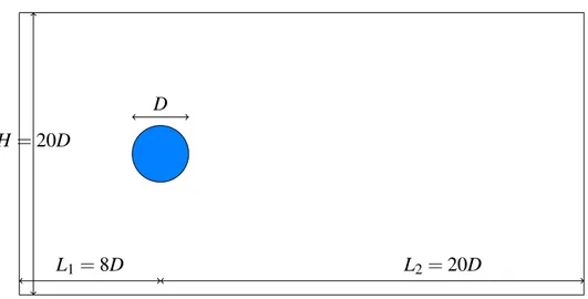
2.2.2 Flow-induced vibration of a free cylinder with Re = 100 . . . 46

3 Numerical investigation on two-phase cross-flow 55

3.1 Selection of a numerical model to use in tube bundle configuration . . . 59

3.1.1 Experiment . . . 60

3.1.2 Sensitivity to the mesh refinement . . . 61

3.1.3 Numerical Investigation . . . 63

3.2 Investigation on the mixtures used in experiments . . . 73

3.2.1 Two-phase flow around a cylinder, literature review . . . 75

3.2.2 Influence of void fraction on the force around a cylinder for a steam-water flow . 77 3.2.3 Parameters of influence for a dispersed flow around a cylinder . . . 79

3.2.4 Impact of the mixture on the force around a tube . . . 84

4 Industrial application: Simulating vibration induced by two-phase flow in a tube bundle 91 4.1 Flow characteristics . . . 92

4.1.1 Bubbly flow . . . 93

4.1.2 Churn flow . . . 94

4.2 Fluid-structure interaction in an in-line tube bundle . . . 101

4.2.1 Vibration of a single-tube induced by a single-phase flow across a 7x7 tube-bundle102 4.2.2 Vibration of a single-tube induced by a two-phase flow across a 7x9 tube-bundle 103 Conclusion and Perspectives 107 Bibliography 109 Appendix A Two-phase flow modeling with NEPTUNE_CFD 117 A.1 Toward two-phase flow numerical modeling . . . 117

A.2 Two-fluid approach . . . 118

A.3 Dispersed approach - Spherical bubbles . . . 119

A.3.1 Drag force . . . 120

A.3.2 Lift force . . . 120

A.3.3 Added mass force . . . 121

A.3.4 Turbulent dispersion . . . 121

A.4 Continuous approach - Large interfaces . . . 121

A.4.1 Large Interface Model . . . 122

A.4.2 Large Bubble Model . . . 123

A.5 Multi-regime approches . . . 124

A.5.1 Generalized Large Interface To Dispersed approach . . . 124

A.5.2 Multi-field approach . . . 125

1 a) Pressurized Water Reactor sketch (source: World Nuclear Association). b) Cross-sketch of an EPR steam generator. The production of steam is Cross-sketched by blue to red arrows. Vibration due to cross flows are located in the red circles. . . 2

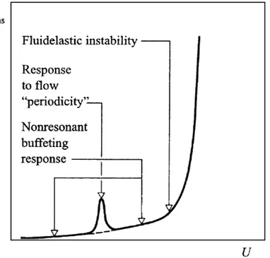
2 Generic idealized response with increasing flow reduced-velocity of a structure, Païdous-sis(2006). . . 3

3 Downstream vortices of a cylinder (Weaver et al.,1993). . . 4

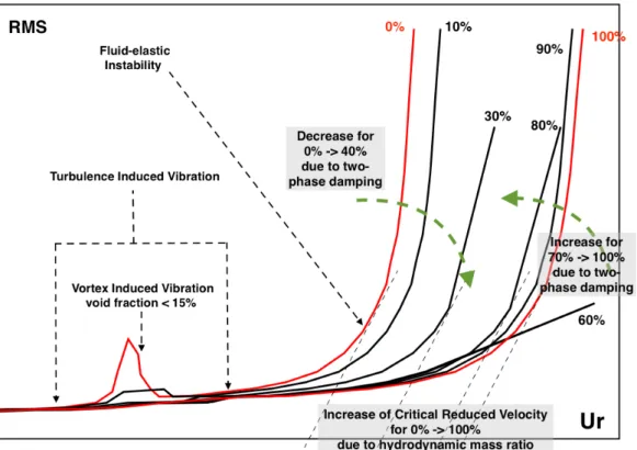
4 Void fraction influence on the structure response with increasing flow reduced-velocity. 5

5 a) Comparison between the theoretical model of hydrodynamic mass (Rogers et al.,1984) with experimental data. The decrease of the hydrodynamic mass is responsible of the increase of the critical reduced velocity. b) Comparison between the theoretical model fromPettigrew(1995) and experiments for different mixtures and configurations. The variations of two-phase damping with void fraction are responsible for the variation of the slope of fluid-elastic departure. . . 5

1.1 A kinematically driven propeller spins with a number of attached Chimera grids. The grids move and rotate with the rigid body frame of the propeller. (English et al.,2013) . 11

1.2 Cut-cell approach, sketch of the different steps of the method. Moreover, each flux from faces concerned in the merging is re-defined. . . 12

1.3 Cell-porosity computation: nodes in the solid domain are in red, others in black. In a cell, if each node is solid (blue), it is a solid-cell; if each node is not solid (white), it is a fluid-cell; otherwise it is a a cut-cell (green). . . 15

1.4 Fluid-structure interface crossing a face in a two-dimensional configuration. Each cell area is calculated by using triangle and rectangle areas when it is required. . . 16

1.5 Decomposition of the domain according to the position of each cylinder. In each subdo-main, the solid velocity is taken equal to the corresponding solid. . . 17

1.6 Fluid-structure interface crossing a cell face. Sub-cycles are required in this case to approximate step by step the value of the face-porosity. . . 18

1.7 Cell crossed by the fluid-structure interface, geometric characteristics re-shaping. . . . 20

1.8 Sketch of the cell center displacements. . . 20

1.9 Sketch of the face center displacements. . . 21

1.10 Iterative determination of the cell centers. Initial positions are represented with bullets. . 21

1.11 Geometric points representation for an inclined channel. . . 23

1.13 Sketch (left) of the Taylor-Green vortices around an immersed square solid with slip walls and numerical results for 5 grid refinements (right). . . 25

1.14 Definition of the characteristic wake dimensions for the steady flow over a stationary circular cylinder (left) and numerical streamlines for Re = 40. . . 26

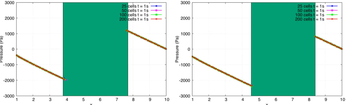
1.15 Pressure profile after discovering a cell (accelerating solid) after 1s (left) and 2s (right). The solid is in green. . . 26

1.16 Geometry of cylinder at fluid velocity case (left) and velocity error for a cylinder at fluid velocity in single and two-phase flow ( with 2 approaches : dispersed and continuous), (right). . . 27

1.17 Geometry of the cylinder suddenly stopped case (left) and drag coefficient around the cylinder moving with Re = 40 and suddenly stopped. Numerical results are compared with other methods (Koumoutsakos and Leonard,1995;Bergmann et al.,2012) (right). 28

1.18 Vorticity isolines for 8 different times with numerical simulation (left) and experimental data (right) fromKoumoutsakos and Leonard(1995) . . . 29

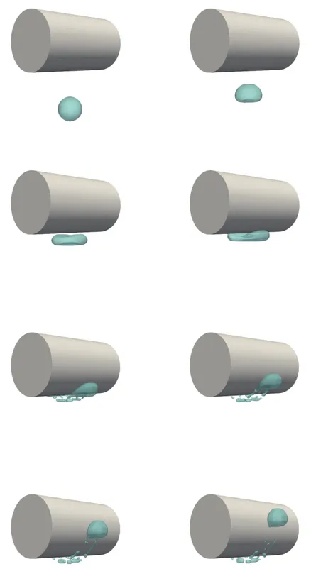
1.19 Geometry of the bubble impact on a cylinder case. . . 30

1.20 Contour comparison of a bubble impacting a cylinder between NEPTUNE_CFD with a

body-fitted mesh and the Time and Space Dependent Porosity method at t = 0.01, 0.1, 0.2, 0.3, 0.4, 0.5, 0.6, 0.7 s. 30

1.21 Snapshots of a bubble impacting a cylinder with the Time and Space Dependent Porosity method at t = 0.01, 0.1, 0.2, 0.3, 0.4, 0.5, 0.6, 0.7 s. . . 31

1.22 Sketch of the tank (Janosi et al.,2004). . . 32

1.23 Experiment/Numerical simulation confrontation of a dam-break on wet bed for d = 18 mm. 32

1.24 Geometry of the wave tank case, (Gao,2003). . . 33

1.25 Free surface evolution for 2 different positions 0.65 m (left) and 5.45 m (right). Compari-son between experiment (Gao,2003) and numerical results from TSDP. . . 33

1.26 Two-phase flow in a centrifugal pump. Air and water are injected by the bottom. The mesh is a box with uniform cartesian cells. The porosity defines the blades and the boundaries of the domain. . . 35

2.1 Fluid-structure interaction with partitioned approach, the explicit or weak coupling. . . 38

2.2 Fluid-structure interaction with partitioned approach, the iterative implicit or strongly coupling. . . 38

2.3 Sketch of the iterative determination of the structure displacement due to the fluid forces. 41

2.4 Cylinder removed from its equilibrium position in a still fluid, geometry. . . 43

2.5 Cylinder removed from its equilibrium position in a still fluid after 1 period on the left, after 31 periods on the right, sub-cycles and δmaxsensitivity. . . 44

2.6 Cylinder removed from its equilibrium position in a still fluid, time step sensitivity. . . 45

2.7 Cylinder removed from its equilibrium position in a still fluid, mesh sensitivity. . . 46

2.9 Mesh utilized for the flow-induced vibration case with Re = 100. On the left, the entire mesh is presented. On the right, a zoom is realized in the zone of interest where the cylinder is. This area is large since the refinement must remain the same whatever the cylinder displacement. . . 47

2.10 Flow-induced vibration at Re = 100 for m∗= 1.25 and k∗= 2.48. Picture of the cylinder displacement and a vortex shedding over time. In this case, the amplitude of displacement is 60% of the diameter. . . 48

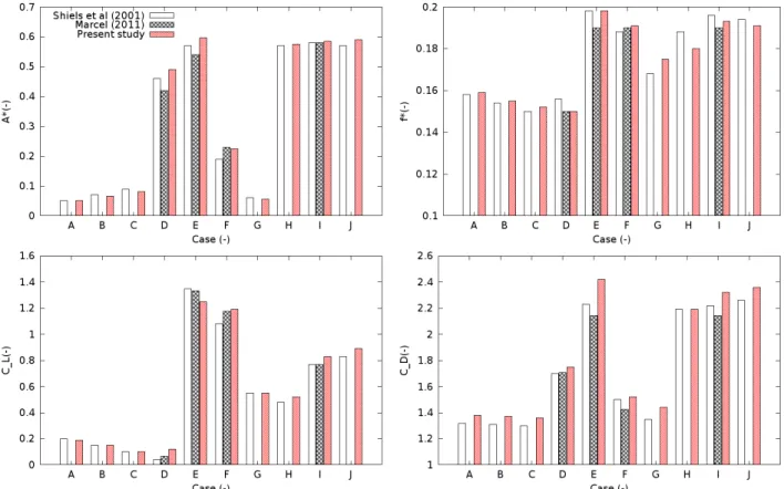
2.11 Response for undamped systems for various cases: A∗ amplitude, f∗ frequency, CL

max lift coefficient and CD,av averaged drag coefficient. Comparison between numerical

results fromShiels et al.(2001),Marcel(2010) and the present method. . . 49

2.12 Response for undamped systems plotted against effective elasticity. Comparison between numerical results fromShiels et al.(2001) and the present method. . . 49

2.13 Confined cylinder released in a fluid, geometry. . . 50

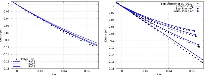
2.14 Free-fall of a sphere on a free-surface: mesh refinement for teflon (on the left). Numeri-cal/experimental displacement along time of a sphere free-falling on a free surface for 4 different materials (on the right). . . 51

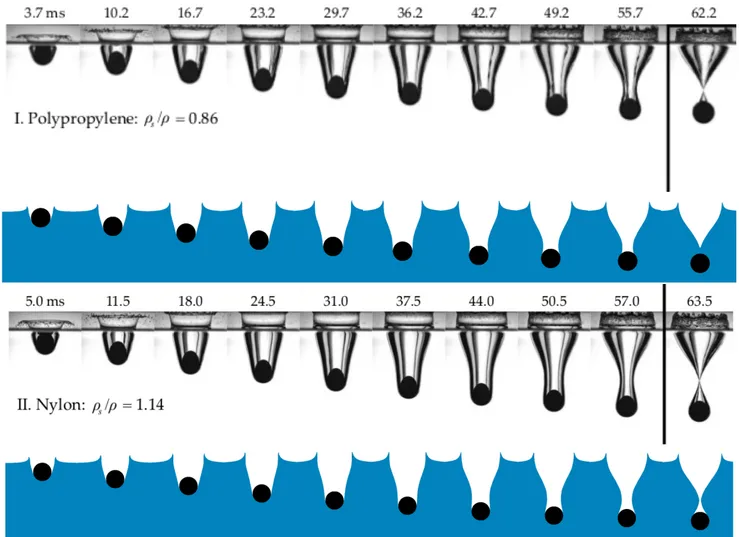
2.15 Polypropylene and nylon spheres falling on a free surface of water. Numerical (bottom) and experimental (top) snapshot of the sphere entry in water. . . 52

2.16 Teflon and steel spheres falling on a free surface of water. Numerical (bottom) and experimental (top) snapshot of the sphere entry in water. . . 53

3.1 Pictures (from the top to the bottom) and flow pattern sketches of bubble, dispersed, large bubbles, churn, intermittent and annular air/water flows in a staggered tube bundle

Kanizawa and Ribatski(2016) . . . 56

3.2 Picture of a bubbly and churn flow in in-line tube bundle,Murakawa et al.(2016). . . 57

3.3 Flow regime map comparison for two-phase flow across a staggered tube bundle.Ulbrich and Mewes(1994) (line) andNoghrehkar et al.(1999) (dash). . . 57

3.4 Influence of the surface tension on the bubble size,Pettigrew and Knowles(1997). For two different inlet void fractions, the bubble diameter is reduced by lowering the surface tension. . . 59

3.5 Inclined tube bundle experiment (Soussan et al.,2001). In blue and green, North/South and West/East planes are colored. . . 61

3.6 Snapshot of the mesh of the tube bundle. It is presented in 2D for only a few tubes in order to see the refinement around tubes . . . 62

3.7 Numerical result using the Generalized Large Interface Model with a Ri j-ε SSG

turbulence model for three mesh refinement called Grid 1, Grid 2 and Grid 3. Averaged void fraction and gas velocity along North/South and West/East lines compared with experimental data. . . 62

3.8 Numerical result using the available numerical models from NEPTUNE_CFD. Averaged void fraction and gas velocity along North/South and West/East lines compared to experimental data. . . 63

3.9 Numerical result using the Generalized Large Interface Model with a Ri j-ε SSG

turbulence model taking into account a surface tension force. Averaged void fraction and gas velocity along North/South and West/East lines compared to experimental data. 66

3.10 Numerical results using the dispersed approach with a Ri j-ε SSG turbulence model

with constant or variable bubble diameters. Averaged void fraction and gas velocity along North/South and West/East lines compared to experimental data. . . 67

3.11 Numerical result using the Generalized Large Interface Model with different turbu-lent models. Averaged void fraction and gas velocity along North/South and West/East lines compared to experimental data. . . 68

3.12 Numerical result using the Generalized Large Interface Model with a Ri j-ε SSG

turbulence model. From left to right: instantaneous void fraction distribution on NS plane, averaged void fraction distribution on NS plane, instantaneous void fraction distribution on OE plane and averaged void fraction distribution on OE plane. . . 70

3.13 Numerical result using the Multi-Fields approach with a Ri j-ε SSG turbulence model.

From left to right: instantaneous void fraction distribution on NS plane, averaged void fraction distribution on NS plane, instantaneous void fraction distribution on OE plane and averaged void fraction distribution on OE plane. . . 70

3.14 Numerical result using the Generalized Large Interface Model taking into account the surface tension force with a Ri j-ε turbulent model. From left to right:

instanta-neous void fraction distribution on NS plane, averaged void fraction distribution on NS plane, instantaneous void fraction distribution on OE plane and averaged void fraction distribution on OE plane. . . 71

3.15 Numerical result using the Generalized Large Interface Model without any turbulent model. From left to right: instantaneous void fraction distribution on NS plane, averaged void fraction distribution on NS plane, instantaneous void fraction distribution on OE plane and averaged void fraction distribution on OE plane. . . 71

3.16 Numerical result using the Generalized Large Interface Model with a k-ε turbulent model. From left to right: instantaneous void fraction distribution on NS plane, averaged void fraction distribution on NS plane, instantaneous void fraction distribution on OE plane and averaged void fraction distribution on OE plane. . . 72

3.17 Numerical result using the dispersed approach with a Ri j-ε SSG turbulence model.

From left to right: instantaneous void fraction distribution on NS plane, averaged void fraction distribution on NS plane, instantaneous void fraction distribution on OE plane and averaged void fraction distribution on OE plane. . . 72

3.18 Numerical experiment for the inclined tube-bundle experiment with freon/freon (top view) and air/water (bottom view). Instantaneous and time-averaged void fraction are present in the NS and WE plane. . . 74

3.19 Picture of bubbly flow around a cylinder for Dcylinder = 40 mm, α0 = 8 %, and

U₀ = 0.45, 0.9, 1.9 m/s from left to right,Inoue et al.(1985). . . 75

3.20 Evolution of the reference equivalent spectra versus frequency for different inlet void fraction, (Pascal-Ribot and Blanchet,2007). . . 76

3.21 . . . 77

3.22 Drag and lift force spectrum for four different inlet void fraction (respectively left and right). . . 78

3.23 Drag (left) and lift (right) force records along time for 0-5% (top) and 10-20% (bottom) of void fraction. . . 79

3.24 Drag (left) and lift (right) force records along time for 50-80% (top) and 90-100% (bottom) of void fraction. . . 80

3.25 Averaged void fraction distribution around a cylinder with αinlet = 8%, Uinlet = 0.9m/s

and D = 40 mm. From left to right, there are experimental data, mesh 1, mesh 2 and mesh 3. . . 81

3.26 Averaged void fraction distribution around a cylinder with αinlet = 4%, 15%, Uinlet =

0.9 m/s and D = 40 mm. From left to right, there are experimental data for αinlet = 4%

and its simulation, αinlet = 15% and its simulation. . . 81

3.27 Averaged void fraction distribution around a cylinder with αinlet = 8%, Uinlet =

0.45, 1.9 m/s and D = 40 mm. From left to right, there are experimental data for U_inlet = 0.45 m/s and its simulation, Uinlet = 1.9 m/s and its simulation. . . 82

3.28 Averaged liquid (left) and gas (right) velocity distribution around a cylinder with αinlet =

8%, Uinlet = 0.45 (top), 1.9 (bottom) m/s and D = 40 mm. . . 83

3.29 Averaged void fraction distribution around a cylinder with αinlet = 8%, Uinlet = 0.9 m/s

and D = 40 mm. From left to right, σ = 0.017, 0.035, 0.075 N/m2. . . 84

3.30 Pictures of the final bubble shape for case B and D from BHAGA . . . 85

3.31 Geometry of the bubble rise (left) and the bubble impact on a cylinder (right) cases. . . 85

3.32 Bubble velocity from numerical simulation along the time for case B and D. . . 86

3.33 Bubble shape comparison between experiment and numerical result for case B. The bubble is in 3D with an opacity of 50%. . . 86

3.34 Bubble impact on a cylinder with two mesh refinements. . . 87

3.35 Snapshots of the impact of the bubble from case B on a cylinder at 4 different times. . . 88

3.36 Snapshots of bubble from case B (left) and D (right) before impact. . . 88

3.37 Forces on the cylinder for case B (left) and D (right). Drag and lift forces are respectively in red and blue. For the case B, the forces computed with the two meshes are in agreement. 89

4.1 VISCACHE tube bundle geometry for single-phase flow (left) and two-phase flow (right). Rigid tubes are filled in white and flexible tubes in black. . . 92

4.2 Void fraction distribution across the tube bundle for water/freon (left) and water/steam (right) for equivalent inlet volume flow rates with a 10% inlet void fraction. The half left of each tube bundle is presented with a volume distribution and the half right with a surface distribution on a slice. . . 93

4.3 Void fraction distribution across the tube bundle for water/freon (left) and water/steam (right) for equivalent inlet mass flow rates with a 10% inlet void fraction. The half left of each tube bundle is presented with a volume distribution and the half right with a surface distribution on a slice. . . 94

4.4 Void fraction distribution across the tube bundle for water/freon (left) and water/steam (right) for equivalent inlet volume flow rates with a 50% inlet void fraction. The half left of each tube bundle is presented with a volume distribution and the half right with a surface distribution on a slice. . . 95

4.5 Void fraction distribution across the tube bundle for water/freon (left) and water/steam (right) for equivalent inlet mass flow rates with a 50% inlet void fraction. The half left of each tube bundle is presented with a volume distribution and the half right with a surface distribution on a slice. . . 96

4.6 Comparison of (from top to bottom) time-averaged void fraction, time-averaged stream-wise liquid velocity, time-averaged transverse liquid velocity and instantaneous bubble diameter along the different rows of the tube bundle. Results are respectively on the left and right for water/freon and water/steam for a 10% inlet void fraction with equivalent volume flow rates. . . 97

4.7 Comparison of (from top to bottom) time-averaged void fraction, time-averaged stream-wise liquid velocity, time-averaged transverse liquid velocity and instantaneous bubble diameter along the different rows of the tube bundle. Results are respectively on the left and right for water/freon and water/steam for a 10% inlet void fraction with equivalent mass flow rates. . . 98

4.8 Comparison of (from top to bottom) time-averaged void fraction, time-averaged stream-wise liquid velocity, time-averaged transverse liquid velocity and instantaneous bubble diameter along the different rows of the tube bundle. Results are respectively on the left and right for water/freon and water/steam for a 50% inlet void fraction with equivalent volume flow rates. . . 99

4.9 Comparison of (from top to bottom) time-averaged void fraction, time-averaged stream-wise liquid velocity, time-averaged transverse liquid velocity and instantaneous bubble diameter along the different rows of the tube bundle. Results are respectively on the left and right for water/freon and water/steam for a 50% inlet void fraction with equivalent mass flow rates. . . 100

4.10 Root-mean-square amplitude of cylinder motion (left) and dominant Strouhal number St= f d/Ug(right) as functions of the gap velocity Ugfor lift direction only. Comparison

of the results from the present study,Granger et al.(1993) andBerland et al.(2014) . . 102

4.11 Tube frequency (left) and root-mean-square amplitude of cylinder motion (right) as functions of the homogeneous velocity Ug for a bubbly flow. Comparison for lift

direction only of the results from the present study, andDelenne et al.(1997). . . 103

4.12 Tube frequency (left) and root-mean-square amplitude of cylinder motion (right) as functions of the homogeneous velocity Ugfor a churn flow. Comparison for lift direction

only of the results from the present study, andDelenne et al.(1997). . . 103

4.13 a) VISCACHE tube bundle geometry for single-phase flow (left). Rigid tubes are filled in white and flexible tubes in black. b) Displacement of the center tube for a unique mobile tube and mobile flexible cell of 9 tubes. . . 104

A.1 Sketch of a dispersed approach. . . 119

A.2 Large interface approach. . . 121

A.3 Three cell stencil. . . 122

A.4 Sketch of the multi-regime approach. . . 124

1.1 Comparison between experimental results (with an “*”), other simulations and the present

study for a cylinder at Re = 40. . . 26

2.1 Cylinder removed from its equilibrium position in a still fluid, numerical and experimental prediction of frequency and reduced damping comparison. . . 45

2.2 Force coefficients and Strouhal prediction for a single-phase flow around a cylinder with Re= 100. Comparison between results fromPomarede et al.(2010) and the present study. 47 2.3 Numerical cases fromShiels et al.(2001) computed in the present study. . . 48

2.4 Numerical and experimental pinch-off time comparison. . . 51

3.1 Comparison of mixtures used in experiment in terms of physical properties. . . 58

3.2 Hierarchy of mesh refinement used for the sensitivity study. . . 61

3.3 Sensitivity to the time of computation depending on the two-phase numerical model. The cluster that was used is an Atos-bull cluster equipped with Intel@Xeon CPU E5 2680 v4 @ 2.40 GHz (Broadwell) nodes with 28 cores. . . 66

3.4 Physical properties of a bubble rise for case B and D fromBhaga and Weber(1981). . 85

4.1 Physical properties of water (1 bar), freon-water (7 bar) and steam generator operating condition: steam-water (70 bar). . . 92

Roman characters

a_0...7 Newmark coefficients (−)

C Damping N.s/m

C_d,Ck Coupling coefficient (−)

CD,CL Drag and lift coefficient (−)

Dor d Diameter m dt, ∆t Time step s Eo Eotvos number (−) F Force N f Frequency Hz g Gravity m/s2

I∗ Displaced cell center (−)

k Phase indicator (−) K Stiffness N.m L Length m l, g Liquid or gas (−) M Mass kg M Momentum transfer N Mo Morton number (−)

n face unit normal vector (−)

P Pressure Pa

R Radius m

Re Reynolds number (−)

SI Surface of cell I m2

t Time s T Temperature K U or u Velocity m/s We Weber number (−) x, y, z Space coordinates m

Greek characters

α Phase fraction (−)

β Solid fraction during sub-iteration (−)

δ Convergence parameter (−)

ε Porosity (−)

γ or β Newmark stability coefficient (−)

µ Viscosity Pa.s Ω Volume m3 ω Pulsation rad/s φ Flux m/s ρ Density kg/m3 σ Surface tension N.m2 τ Reynolds-stress tensor N

θ Value between 0 and 1 (−)

ξ Reduced damping (−)

Acronyms

CEA Commissariat à l’Energie Atomique CFD Computational Fluid Dynamics DNS Direct Numerical Simulation

EDF Électricité de France FEI Fluid Elastic Instability FSI Fluid-Structure Interaction

GLIM Generalized Large Interface Model

IBM Immersed Boundary Method

IRSN Institut de Radioprotection et de Sureté Nucléaire

LBM Large Bubble Model

LES Large Eddy Simualtion LIM Large Interface Model

NS North South

PWR Pressurized Water Reactor

RANS Reynolds-Averaged Navier-Stokes

RMS Root Mean Square

SG Steam Generator

TSDP Time and Space Dependent Porosity VIV Vortex Induced Vibration

1. W. Benguigui, J. Laviéville, S.Mimouni, N. Mérigoux, E. Longatte, First steps in the development of an eulerian fixed grid postulation for two-phase flow-induced vibration numerical modeling, Flow Induced Vibration, La Haye, Pays-Bas, 2016.

2. W. Benguigui, J. Laviéville, S.Mimouni, E. Longatte, Suivi d’une interface solide mobile au sein d’un écoulement diphasique par une méthode de frontière immergée, CSMA, Gien, 2017.

3. W. Benguigui, E. Deri, J. Laviéville, S.Mimouni, E. Longatte, Numerical experiment on two-phase flow behaviors in tube bundle geometry for different mixtures, Pressure Vessels and Piping, Waikoloa Village, Hawai USA, 2017.

4. W. Benguigui, E. Deri, J. Laviéville, S.Mimouni, E. Longatte, Numerical investigation and analysis of a dispersed two-phase flow across a single rigid cylinder, Flow Induced Vibration, Toronto, Canada, 2018.

5. W. Benguigui, E. Deri, J. Laviéville, S.Mimouni, E. Longatte, Numerical investigation of a single bubble impacting a cylinder, fist steps towards the up-scaling, Flow Induced Vibration, Toronto, Canada, 2018.

6. W. Benguigui, A. Doradoux, J. Laviéville, S. Mimouni, E. Longatte, A discrete forcing method dedicated to moving bodies in two-phase flows, International Journal for Numerical Methods in Fluids, 2018 .

In thermal power stations, the generated heat is used to boil water in order to drive a steam turbine connected to an electric generator. In nuclear pressurized water reactors (Pressurized Water Reactor), the heat is generated in the core and carried out by a primary liquid water circuit. Then, via a tubular heat exchanger, called steam generator, power is transferred to a boiling secondary water circuit (see Figure1

a)). This hence produced steam is dried before entering the turbine.

There are three or four steam generators per reactor in France. They can measure up to 20 m and weigh as much as 800 tons. They can contain from 3000 to 16 000 U-tubes with a diameter of approximately 20 mm. A sketch of the EPR steam generator is proposed in Figure1b) : this type of power plan will start soon to produce power in France. In typical PWR recirculating steam generators, the primary system coolant flows through U tubes with a tube sheet at the bottom of the generator and U bends at the top of the tube bundle. Primary coolant enters the steam generator usually at 315 - 330oC on the hot leg side and leaves at about 288oC on the cold leg side. The secondary system water is fed through a feedwater nozzle, to a feedwater distribution ring, into the downcomer, where it mixes with recirculating water draining from the moisture separators. This downcomer water flows to the bottom of the steam generator, across the top of the tube sheet, and then up-wards through the tube bundle, where steam is generated. About 25% of the secondary bulk water is converted to steam as it passes through the tube bundle up-wards, the remainder is recirculated.

As steam generators degrade over time, their integrity is extremely important both for economic and safety reasons. Consequently, during scheduled maintenance outages or shutdowns, steam generator tubes are inspected. If necessary a tube might be plugged to remove it from operation. The French regulatory agency requires a baseline inspection of all tubing full length before operation, periodic inspections at least every two years, and complete inspections (presumably 100% of the tubes full length) every ten years. The tube support plate and sludge pile inspections might also be realized.

Steam generator problems may constrain the plants to perform unscheduled or extended maintenance operations. Unfortunately, steam generator maintenance and replacement are expensive and the origins of the degradations are multiple. The present work is motivated by one of the main ones: flow induced vibration of heat exchanger tubes. This phenomenon might be seen in two different locations of the steam generator (Pettigrew and Taylor,2003) where there is a cross-flow : at the bottom of the bundle under single-phase flow and at the top under two-phase flow with high void fractions (see Figure1b)). At the bottom of the bundle, it is a single phase flow. Two kinds of degradation mechanisms may be generated by flow induced vibration: fretting wear and high cycle fatigue. Anti-vibration bars, tube support plates or tubes might be affected by these mechanisms. In general, before having leakage or rupture problems, tubes are plugged in order to put them out of service. However, few nuclear power

Figure 1 a) Pressurized Water Reactor sketch (source: World Nuclear Association). b) Cross-sketch of an EPR steam generator. The production of steam is sketched by blue to red arrows. Vibration due to cross flows are located in the red circles.

plants abroad reported tube ruptures. Consequently, flow induced vibration, being a major concern for the correct steam generator behavior, has been studied in order to understand and prevent this phenomenon.

According to Price(1995), cross-flow induced vibration mechanisms are indexed in three main categories: Tubulence-Induced-Vibrations (TIV); Vortex-Induced-Vibrations (VIV); Fluid-Elastic Insta-bility (FEI) or Motion-Induced-Vibrations (MIV). Experimental data from literature illustrating vibration regimes according to the flow velocity highlight distinctly three different ranges of vibrations.

Figure 2 Generic idealized response with increasing flow reduced-velocity of a structure,Païdoussis

(2006).

A solid body immersed in a fluid flow is subjected to random turbulent forces given by the pressure fluctuation at the wall: this results in TIV vibration. It is possible to model the object as a filter taking energy from the fluid. In fact, the solid begins to vibrate with a slight amplitude. These vibrations are more or less large depending on the Reynolds number. For a steam generator, turbulence is essential to stimulate heat transfer. Even if this phenomenon leads to low vibration magnitudes, it is vital to take it into account because of its influence on the tube duration.

The wake downstream of the cylinder produces periodic vortices on both tube sides (see Figure3). The structure is not impacted by the shedding as long as the vortex shedding frequency is different from the natural frequency of the tube. When these frequencies are close, a peak is observed in response amplitude (see Figure.2). VIV is stable thanks to the non-linearities of the system .

Fluid-elastic instability is the most violent phenomenon for the structure as it might cause damages. In fact, it is the result of hydrodynamic forces which originate as a result of the vibration itself. The larger the amplitude of vibration, the larger the force, consequently vibration amplitude increases with velocity. This self-amplified phenomenon appears above a critical velocity and most of the time leads to tube failure. Therefore, fluid-elastic instability is of major concern for industry especially nuclear power plants. Many studies have been performed in order to predict FEI critical velocity for decades (Langre,

Figure 3 Downstream vortices of a cylinder (Weaver et al.,1993).

In reality, two-phase cross flows appear in more than half of the heat exchangers utilized in industry (Green and Hestroni,1995; Noghrehkar et al., 1999). Consequently, the phenomenon is even more challenging since void fraction and two-phase flow regime affect the dynamic parameters of the tube. The two-phase character of the problem is therefore of primary interest. For bubbly flows, under 20% of void fraction, the response of the tube is similar to the one in single phase flow. By increasing the void fraction, the critical reduced velocity is increased according toDeri(2018). The higher the void fraction, the lower the VIV intensity. Between the bubbly and the intermittent flow, the regime transition is characterized by the decrease of the fluid-elastic departure (see green arrow in Figure.4). During the intermittent flow, between 30% and 70% of void fraction, the fluid-elastic slopes are low (see the response for α = 60% in Figure.4), probably because of the mix of small and large gas structures. Then, for more than 70% of void fraction, the slope increases with void fraction (green arrow in Figure.4). Beyond 85%, the curve of the RMS depending on the velocity is unchanged. These phenomena are observed on different experiments with different mixtures and mass flow rates. Based on the influent parameters such as the array orientation for example, different authors tried to explain the reason why the vibration are highly different depending on the flow pattern.

In a heat exchanger, the dynamic response of a tube is characterized by its inertia, stiffness and damping. Illustrated in different experimental studies, these two-phase dynamic parameters (added mass and damping only) are different from single-phase flow ones which is consistent since damping and hydrodynamic mass in single phase flows depend on fluid properties.

Added mass is defined as the equivalent mass of external fluid vibrating with the structure (Pettigrew and Taylor,1994). In two-phase flow across a tube, hydrodynamic mass decreases linearly with void fraction increment as seen in Figure5a). This is relevant since it would explain the increase of critical reduced velocity when void fraction increases.

Damping is responsible of the energy dissipation of the system. In two-phase flow, there is a strong dependency on void fraction as seen in Figure 5 b). For intermediate void fraction, consequently intermittent regime, the damping reaches a maximum. The relationship between local void fraction fluctuations and damping ratio makes sense, since there are large temporal fluctuations in the momentum

Figure 4 Void fraction influence on the structure response with increasing flow reduced-velocity.

Figure 5 a) Comparison between the theoretical model of hydrodynamic mass (Rogers et al.,1984) with experimental data. The decrease of the hydrodynamic mass is responsible of the increase of the critical reduced velocity. b) Comparison between the theoretical model fromPettigrew(1995) and experiments for different mixtures and configurations. The variations of two-phase damping with void fraction are responsible for the variation of the slope of fluid-elastic departure.

whenever gas and liquid slugs alternatively impinge on the vibrating tube in intermittent flow. Damping is responsible for the variation of the fluid-elastic instability departure proposed in Figure4.

Since a major knowledge has been shared from experiments, the numerical prediction of fluid-elastic instability has been investigated. It requires a fluid-structure interface tracking method to follow the motion, high resolution of the turbulence in order to predict correctly hydrodynamic forces at the wall and a robust coupling algorithm to avoid numerical issues. When the motion is computed based on fluid forces acting on the cylinder, the method is called “Direct Numerical Flow-Structure coupled CFD”. Tubes are allowed to move freely according to the load at wall. Each tube is considered by a mass/damping/stiffness system. Using Large Eddy Simulation to correctly model turbulence and Arbitrary Lagrangian Eulerian method (described in other sections) to displace tubes, the direct approach might be time-consuming but representative of experiments.Pedro et al.(2016);Shinde et al.(2014) are examples that successfully utilized this approach in simulating flow in tube-bundles. An other method consists in imposing the displacement of a single tube, recording the fluid forces on this tube and the surroundings to predict the instability based on theoretical models (Hassan et al.,2010;Bouzidi et al.,2014). A major knowledge has been shared for years on vibrations induced by single-phase flows. Influent parameters have been studied in details. Nowadays, the objective of the present work is to address vibrations induced by two-phase flows.

Two-phase flow induced vibration phenomenon is more complex. Reduced-scale experiments were performed to characterize the flow patterns and the vibrations. Most of the time, modeling mixtures are used since an experiment with steam and water is expensive. However, an effort is made to use fluids having similar fluid properties. In contrast to single-phase flow, this phenomenon has not really been investigated with numerical simulation. Only few studies based on strong assumptions (using 2D simulation, with fixed bubble diameter, with a RANS turbulence model) were performed (Sadek et al.,

2018). By imposing motion, results are in correct agreement with the experiment, however to predict the motion results are not accurate between 10% and 90% of void fraction, consequently in two-phase flow. Since the maturity of two-phase flow numerical simulation allows to perform multi-regime flows, it is now time to deal with two-phase flows in order to complete and enforce the knowledge coming from experiments.

Organization of the present manuscript

Simulating gas-liquid flows involving a wide range of spatial and temporal scales and multiple topological changes remains a major challenge nowadays. Computational cost associated with direct numerical simulation still being unaffordable, the two-fluid Euler-Euler approach is a proper way to compute such kind of flow. The present work is dedicated to the simulation of two-phase flow induced vibration with the code NEPTUNE_CFD detailed in appendix A. Organized in four parts presented below, the manuscript begins by describing the required developments to perform fluid structure interaction in the code before going through two-phase flow across tube bundle and the prediction of the fluid-elastic instability threshold on the VISCACHE experiment.

1. Time and Space Dependent Porosity method: the numerical simulation of interactions between immersed structures and two-phase flows requires an accurate fluid-structure interface tracking method. In the present work, a discrete forcing method based on a porous medium approach is

proposed to follow non-deformable rigid body with an imposed velocity by using a finite-volume Navier-Stokes solver dedicated to multi-phase flows and based on a two-fluid approach. To deal with the action reaction principle at the solid wall interfaces in a conservative way, a porosity is introduced allowing to locate the solid and insuring no diffusion of the fluid-structure interface. The volumetric fraction equilibrium is adapted to this novelty. Mass and momentum balance equations are formulated on a fixed cartesian grid. Interface tracking is addressed in detail going from the definition of the porosity to the changes in the discretization of the momentum balance equation. This so-called Time and Space Dependent Porosity (TSDP) method is then validated by using analytical and elementary test cases. Finally, a feasibility study is performed to predict the flow patterns in a centrifugal pump.

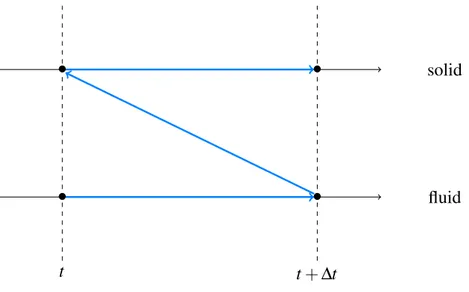
2. Fluid Structure Interaction with the Time and Space Dependent Porosity method The fluid-structure coupling is a tough numerical challenge. Depending on the chosen scheme, the prediction of displacement differs since accuracy might require computational time. Even if it is more time-consuming, an iterative algorithm is chosen and detailed. The force computation with the Time and Space Dependent Porosity is detailed since no body-fitted mesh is used. In order to predict the displacement after each iteration, a Newmark algorithm is implemented. The validation of the present fluid-structure coupling is performed on three cases: a cylinder release in a fluid at rest, a single-phase cross-flow around a free-cylinder at Re = 100, and the free-fall of a sphere on a free surface. Finally, the method is applied on an industrial application: the hydraulic dashpot.

3. Numerical investigation on two-phase cross-flow Two-phase flow across tube bundle knowledge comes from experimental and theoretical feedbacks only. In the present section, a fine study is carried out to enhance this knowledge since simulations give access to many informations. First, the numerical models are evaluated to determine the most competitive one. The influence of different numerical and physical parameters is checked. Based on two different mixtures, two-phase flows across tube bundles are numerically explored. Then, in order to have access to fine information, two-phase flow across a single cylinder and the impact of a single bubble on a cylinder are computed. Finally, using the results from each numerical investigation, depending on the mixture physical properties, two-phase cross-flow are described and possible perspectives are given.

4. Industrial application: Simulating vibration induced by two-phase flow in a tube bundle The numerical experiment of changing mixture is performed in order to quantify the error when freon/water is used instead of steam/water. Being able to follow an immersed structure motion induced by a two-phase flow and having determine the required numerical model to use in previous sections, the direct numerical prediction of vibration induced by two-phase flow in an in-line tube bundle is performed. A description of the simulated experiment is realized and numerically studied for rigid cylinder and then for free-cylinders.

Interface tracking method dedicated to

moving bodies in two-phase flow

1.1

Interface tracking method dedicated to fluid-structure

interac-tion

To follow numerically the motion of a structure on a mesh, it is necessary to have a dedicated method. Different kinds of fluid-structure interface tracking methods are found in the literature such as Arbitrary Lagrangian Eulerian, Chimera, Immersed Boundary and others. In order to highlight the discrepancies between each one, some are presented in the present section.

Depending on the geometry, amplitude of motion or the required accuracy, one interface tracking method may appear more appropriated than an other. Two kinds of interface-tracking method are distinguished:

• Adaptative grid method (deformation or motion) where the grid is updated along time depending on the motion. It might be adapted to the motion like the (Arbitrary Lagrangian Eulerian (Noh,

1964)), or the mesh dedicated to the solid is moved like in the Chimera (Benek et al.,1983).

• Fixed grid method where the grid is not used to follow the motion. Two ways are consequently possible: having moving boundaries on a body-fitted mesh (Lighthill,1958), or have a dedicated function to follow the solid: Immersed Boundary Method (Peskin,1972;Mittal and Iaccarino,

2005).

1.1.1

Popular interface tracking methods with adaptative grid

A) Arbitrary Lagrangian Eulerian

The Arbitrary Lagrangian Eulerian formalism defines structures and near-wall fluid areas with Lagrangian coordinates, fluid with Eulerian coordinates, and between this two areas with arbitrary coordinates. Here, the grid is body fitted depending on the geometry of the structure. Based on the solid velocity, the grid is deformed or distorted to follow its motion. Consequently, the grid velocity is

dependent from the solid velocity and introduced in fluid dynamic equations. However, far from the structure, in the Eulerian coordinate area, the grid velocity is null; only the near-structure zone is distorted. In the arbitrary area (between Eulerian and Lagrangian areas), an arbitrary velocity is given in order to fit the grid displacements.

Introduced by Noh (1964), the method is fully described in Donea et al. (2004) and different applications are highlighted. In the Arbitrary Lagrangian Eulerian method, computational mesh inside the domains can move arbitrarily to optimize the shapes of elements or to follow the motion of a rigid structure.

The grid update is the key point in this method given that it is required for each time step. Conse-quently, it has to be :

• robust and accurate in order to prevent from having large modification of the mesh topology; • low time-consuming as it is called at each time step.

Unfortunately, there is no algorithm satisfying fully both conditions. In fact, this method is dedicated to slight vibration such as cylinder vibrations in tube bundles since the grid distortion is not important. For example, it is impossible to follow a rotating propeller with an ALE interface tracking method.

However, for flow induced vibration, especially for cylinder or tube bundle, the method has been popular for many years.

B) Chimera/Overset grid

Grid generation is often the limiting factor for industrial simulations. To overcome this problem, some solutions are proposed like the Immersed Boundary Method (IBM) or Chimera method. The last one, chimera method (or also called overset grid method) appears increasingly used for complex research applications and more and more for huge industrial applications.

Initiated byBenek et al.(1983), the principle is to decompose the complex full domain into simple subdomains independently meshed by curvilinear grids. The only constraint is a superposition of grids to allow the link of the flow description. A first step of the process is to detect overlapped cells and to determine if it is an interpolated cell (it means that its flow data are coming from an other grid), a calculated cell (it means that flow data are coming from its own grid), or a cell with no interest for the flow (not interpolated nor calculated). Donor cells and the associated weights that compose the interpolation are evaluated for each valid overlapped cell in order to compute interpolation values. Consequently, two grids that are allowed to communicate by their cells are overlapped. There is no limitation in the number of grids.

Beyond simplifying the mesh generation, this technique offers a powerful solution to deal with moving bodies given. Moreover, a complex geometry is meshed thanks to an assembly of simple grids. This is illustrated in the study ofEnglish et al.(2013).

Figures1.1demonstrates the efficiency of this method for a complex problem. However, its imple-mentation in an existing code is time-consuming and difficult: interpolations, overlapped cell detection, many grids... In the present work, as the geometry may be consider simple (tube bundles), this method appears to not be the most adapted.

Figure 1.1 A kinematically driven propeller spins with a number of attached Chimera grids. The grids move and rotate with the rigid body frame of the propeller. (English et al.,2013)

1.1.2

Immersed Boundary Methods

The term immersed boundary methods is a class of methods devoted to describe accurately moving immersed bodies (such as two-phase flow, or fluid-structure interaction) in a fixed Cartesian grid. Immersed Boundary Method (IBM) consists in representing fluid in an Eulerian framework and solid in a Lagrangian one on a unique mesh. This procedure is less time-consuming and eliminates issues from re-meshing or deforming-mesh, such as the mesh distortions and the mesh interpolation errors in the body-fitted mesh methods (ALE for example). Two categories are identified :

• Continuous forcing: operator discretization is unchanged, however a source term is added in the momentum balance equation in order to take into account the immersed boundary. Penalty method and Peskin approach are continuous forcing methods.

• Discrete-forcing: operator discretization is different close to the fluid-structure interface in order to take into account the boundary. Cut-cell and Ghost-cell are discrete-forcing methods.

A) Continuous forcing methods

Peskin approach This kind of method was first introduced byPeskin(1972) for the simulation of blood flow in human heart. At the beginning, the method was only dedicated to flexible boundaries in motion. By adding a source term in the momentum equation, the boundaries of the immersed body are taken into account. One grid is dedicated to follow the structure with a Lagrangian framework and the other one for the fluid with an Eulerian framework. As the structure grid does not follow the Eulerian one, the interface force is imposed at the nodes.

Penalty methods Arquis and Caltagirone(1984);Caltagirone and Arquis(1986) introduced penalty methods dedicated to fluids mechanics. The concept is to consider a unique equation on the whole domain. A penalty source term, describing the constraint from a subdomain, is added in the momentum balance equation. This term is then multiplied by a penalty parameter dependent on the concerned subdomain. This parameter is here a kind of local permeability: a value of 0 meaning that the subdomain

is the solid, a value of 1 the fluid. For solid in displacement, it serves to impose the solid velocity in its subdomain. Different studies improves the order of the method in the recent years by interpolation of the velocity at the interface from the nodes (Carbou and Fabrie,2003;Sarthou,2009).

B) Discrete-forcing methods

The concept of these methods, in mirror of continuous forcing ones, is to keep unchanged the conservation laws at the wall by modifying the operator discretizations in order to have the right condition at the fluid-structure interface. These methods are robust and used for different situations from bubbly flow to fluid-structure interaction.Bai et al.(2010) used Cartesian cut cell approach to simulate waves for example.

Cut-cell method (Clarke et al.,1986;Ye et al.,1999) This approach modifies the shape of the control volumes near the interface by cutting and merging them. Mass, convective, diffusive fluxes and gradients have to be computed on each face of these new cells. Figure1.2shows how to conform the immersed fluid-structure interface by cutting and merging the concerned cells.

a) Interface-cell recognition b) Cell cutting step c) Cell merging step

Figure 1.2 Cut-cell approach, sketch of the different steps of the method. Moreover, each flux from faces concerned in the merging is re-defined.

Embedded Boundary Method Developed byJohansen and Colella(1998), this approach is similar to the cut-cell method since interface-cells are cut. However, the solution is still calculated at the center of the cell even if it is not in the fluid domain. Fluxes are like in the cut-cell method computed at corrected faces.

Ghost-cell Method Developed byTseng and Ferziger(2003), this approach consists in the introduction of a force in the Navier-Stokes equation in order to impose the exact boundary condition at the fluid-structure interface. For each cell crossed by the interface, a ghost zone is introduced in the non-fluid area where the boundary condition has to be enforced. When the interface is on a node, the velocity at the node is the solid one. For the other situations, the velocity is extrapolated in each ghost-cell in order to get the accurate velocity at the interface.

The major disadvantage of this method is the numerical instability when the interface is close from a node. The extrapolation coefficients are consequently very large and may cause convergence trouble. Two solutions are proposed:

• displace locally the interface position to be accurately on the node, • use the symmetric of the concerned node as the interpolation point.

This method is robust and used for different situations like bubbly flow or fluid-structure interaction. In the following section, a Discrete Forcing method dedicated to moving bodies in two-phase flow is proposed. This is not the first time a work is dedicated to this kind of flow with a discrete-forcing method. For example,Hu et al.(2006) investigated breaking waves, he used the cut-cell method to reproduce the reef. However, most of the time these methods are implemented in multi-phase flow code based on a one-fluid approach. The novelty of the present work is to implement a discrete forcing method in a code based on a two-fluid approach and to adapt the volumetric fraction equilibrium and the momentum balance equation to it.

1.2

Time and Space Dependent Porosity method definition

The present developments are implemented within a finite-volume CFD code dedicated to multiphase flows and based on the two-fluid (extended to n) approach. Using a pressure correction approach (Ishii,

1975), it is able to simulate multiphase flows by solving a set of three balance equations for each field (2 in adiabatic cases): ∂ (αkρk) ∂ t + ∇ · (αkρkUk) = 0 ∂ (αkρkUk) ∂ t + ∇ · (αkρkUkUk) = −αk∇P + αkρkg+ ∇ · τk+ N

∑

p=1 p̸=k M_p→k (1.1)

where α, ρ, U , P, τ, g and M are respectively the volume fraction, the density, the velocity, the pressure, the Reynolds-stress tensor, the gravity and the momentum transfer to the phase k. The k-phase volumetric fraction is written αk. In multiphase flow, one property of the k-phase volumetric fractions is:

N

∑

k=1

αk= 1 (1.2)

with N the number of fluid phases included into the fluid domain.

The aim of discrete forcing methods is to strictly ensure the conservation laws at the close vicinity of the interface. The idea is to reshape the cells crossed by the interface and to build specific schemes inside them. The interface is approximated as a plane in each cut-cell. The domain contains the structure, which is considered as a real part of the calculation domain. A tag function is therefore required to determine the solid location on the cells. The main advantage of these methods lies in the non-explicit

representation of the structure, meaning that it is possible to perform calculations on complex geome-tries using Cartesian grids. The major challenge of these methods is to reconstruct the interface properties.

In order to locate the solid, cells are identified as a solid, fluid, or interface cells. In the present method, the whole domain is considered in the framework of a porous media approach where a time and space dependent fraction called porosity is 0 in the solid, and 1 in the fluid. The fluid-structure interface is consequently represented with a porosity between 0 and 1. Here, the porosity is as follows:

ε (x, t) = 1 − αs(x,t) (1.3)

with αsthe volumetric fraction of the solid phase, and ε(x,t) the porosity (in x at time t) being between

[0, 1]. Therefore, the previous relation (1.2) describing the volumetric fraction balance becomes:

∑

k

αk(x,t) = ε(x,t) (1.4)

This method involves a non-moving Cartesian grid where the body is meshed and defined with a porosity equal to 0 insuring no mass transfer between solid and fluids. In a finite-volume framework, the porosity is computed for a cell I by using the following relation:

εI =

fluid volume of the cell I

total volume of the cell I. (1.5)

Here, the solid motion is tracked thanks to the porosity evolution in a Lagrangian framework. To take into account the solid motion and the presence of an interface in cut-cells, the porosity has to be convected and the momentum balance equations are formulated differently.

1.2.1

Porous mass balance equation and media definition

The time and space dependent porosity definition is the key element in the method. The total volume of the solid domain should be constant whether the object is moving or not. Acting like volumetric fraction, a porosity is computed for each cell and for each face of the domain in order to convect the structure.

A) Cell-porosity computation

Three kinds of cells are possible and defined thanks to the porosity: 1. if the cell is solid, porosity value is 0 ;

2. if the cell is fluid, porosity value is 1 ; 3. in other cases, the cell contains an interface.

At each time step, the porosity is computed by using a Volume of Fluid Initialization (VOFI) method (Bnà et al.,2015b,a) as follows. An implicit function f is introduced. This function is defined as follows :

• • • • • • • • • • • • • • • • • • • • • • • • • • • • • • • • • • • • • • • • • • • • • • • • • • • • • • • • • • • • • • • • • • • • • • • • • • • • • • • • •

Figure 1.3 Cell-porosity computation: nodes in the solid domain are in red, others in black. In a cell, if each node is solid (blue), it is a solid-cell; if each node is not solid (white), it is a fluid-cell; otherwise it is a a cut-cell (green).

solid domain. Then, this function is used in order to evaluate in each cell the porosity. Examples of cells with porosity of 0, 1 and intermediate values are displayed on Figure1.3.

B) Geometric face-porosity determination

If a face is cut by the fluid-structure interface, the two Cartesian neighboring cells sharing this face are required to compute geometrically the face porosity. Based on the node coordinates and the porosity of each cell, it is determined geometrically by assuming the interface to be locally straight (linear function) instead of curved. Several configurations are possible and illustrated in two dimensions in Figure1.4for εI > εJ.

The interface is defined by: y = Ax + B where A and B are two real coefficients. In each cell, the blue surface is computed based on node coordinates, A, B. Consequently, for a given case :

(

S_I = 1 − αI = s1(A, B, x)

S_J = 1 − αJ= s2(A, B, x)

(1.6)

where SI and SJ designate respectively the blue areas of both cells, s1and s2are two functions computing

the area based on A, B and x. The computation of this system leads to an evaluation of A and B, and then εIJ. For example, node coordinates are given in Figure.1.4for case (A). Based on them, the blue surface

is computed in each cell such as: (

S_I = 1 − αI = BL + AL2/2

S_J = 1 − αJ= (AL + B)L + AL2/2

(1.7)

Then, by solving the present system, A and B are computed. Finally, εIJ = 1 − (AL + B). For

• I • J (A) εIJ • (0, 0) (L, 0)• (2L, 0)• • (0, 0) • (L, 0) • (2L, 0) • (0, B) • (L, AL + B) • (2L, 2AL + B) • I • J (B) εIJ • I • J (C) εIJ • I • J (D) εIJ

Figure 1.4 Fluid-structure interface crossing a face in a two-dimensional configuration. Each cell area is calculated by using triangle and rectangle areas when it is required.

C) Convected porosity computation

As described in (1.4): the porosity has to be treated like k-phase volumetric fractions, hence convecting the porosity is necessary. There are no mass transfer between a solid and other phases, therefore:

∂ ε

∂ t + ∇ · (εUs) = 0 (1.8)

with ε = ∑kαk. In a finite-volume framework, the discretization at each time step is given by:

ε_In+1− ε_In

∆t ΩI+_J∈N

∑

I

ε_IJnφIJ = 0 (1.9)

with φIJ = Us· nIJ, where nIJ is the face unit normal vector between cells I and J, and NI neighboring

cells around I. For multiple solids, the domain is decomposed in subdomains depending on the position of each structure in order to differentiate their own velocities like in Figure1.5. In order to allow the independent motion of different structures with several velocities, the solid volumetric phase fraction αs= 1 − ε is convected since it is null outside each structure. The convection equation becomes:

αsn+1_I − αsn_I

∆t ΩI+_J∈N

∑

I

Outside structures, one gets ∑J∈NIφIJ = 0. Given that αs is also null outside solid sub-domains, the convection equation is thus formulated in an equivalent way in order to keep the minimum and the maximum principles true:

αsn+1_I − αsn_I ∆t ΩI+_J∈N

∑

I (αsnIJ− αsnI)φIJ = 0. (1.11) •ω1 •ω2 •ω3 •ω4 U_S1 U_S2 U_S3 U_S4 U_S1 U_S2 U_S3 U_S4

Figure 1.5 Decomposition of the domain according to the position of each cylinder. In each subdomain, the solid velocity is taken equal to the corresponding solid.

To minimize the numerical diffusion and keep positivity and maximum principles for porosity, a θ -scheme is used to define the face porosity fraction, and each time step is subdivided into sub-time step to approximate accurately the face porosity. An example of 2D configuration is given in Figure

3.34. Using a θ -scheme, the porosity is expressed in terms of the current face function αsGEOMand a

decentered value αsU PW INDas follows :

αsIJ= θIJαsGEOMIJ + (1 − θIJ)αsU PW INDIJ (1.12)

with θIJ ∈ [0, 1]. Using an upwind decentered scheme yields : αsU PW IND_IJ = αsI for φIJ > 0 and

αsU PW IND_IJ = αsJ for φIJ < 0. αsU PW IND_IJ ∈ [0, 1]. As far as possible, θIJ is close to 1 in order to

preserve the highest geometric contribution. The UPWIND and geometric face porosity computation are satisfied thanks to a Courant condition on the time step. Introducing the time step subdivision, let i be an integer i ∈ [0, imax] and β the solid fraction during a sub-iteration such that β_I0= αsn_I and β_Iimax = αsn+1_I .

The sub-cycling time step becomes: dt = ∆t

i_max. Therefore, the θ -scheme is used to define β

i

IJ and leads

to the αsnIJ thanks to the relation:

αsnIJ = ∑i∈[0,imax]β i IJ imax . (1.13)

This relation is used to solve iteratively the mass balance equation (1.11). The derivation of the iterative θ -scheme is presented below. For a cell I, lets assume 0 ≤ β_Ii≤ 1 and derive 0 ≤ β_Ii+1≤ 1:

• I

• J

U_s I• J•

Figure 1.6 Fluid-structure interface crossing a cell face. Sub-cycles are required in this case to approximate step by step the value of the face-porosity.

1. Positivity

β_Ii+1− β_Ii

dt ΩI+_J∈N

∑

I

(β_IJi − β_Ii)φIJ = 0

It is possible to formulate the expression by highlighting decentered terms according to the flux sign: β_Ii+1− β_Ii dt ΩI+_J∈N

∑

I,φIJ≥0 (θIJβ_IJi,GEOM+ (1 − θIJ)βIi− βIi)φIJ) +

_∑

J∈NI,φIJ<0 (θIJβIJi,GEOM+ (1 − θIJ)βJi− βIi)φIJ) = 0 One defines A = − ∑J∈NI,φIJ<0(θIJβ i,GEOM IJ + (1 − θIJ)βJi)φIJ) which is positive. β_Ii+1 dt ΩI = β_Ii dtΩI+ A +_J∈N

∑

I,φIJ<0 βIφIJ−

∑

J∈NI,φIJ≥0 θIJ(β_IJi,GEOM− βIi)φIJ

To ensure the positivity of β_Ii+1, the condition is:

∑

J∈NI,φIJ≥0 θIJ(β_IJi,GEOM− βIi)φIJ≤ β_Ii dtΩI+ A +_J∈N

∑

I,φIJ<0 βIφIJ (1.14)

2. Maximum: Let assume β_Ii+1= 1 − ε_Ii+1. To ensure the positivity of ε_Ii+1(consequently β_Ii+1≤ 1), the condition is similarly:

∑

J∈NI,φIJ≥0 θIJ(ε_IJi,GEOM− εIi)φIJ ≤ ε_Ii dtΩI+ A +_J∈N

∑

I,φIJ<0 εIφIJ (1.15)

Therefore, θIJ has to ensure both conditions. θIJ is defined per cell (not per face) as a θI. Thus, the

conditions become for a cell I:              θI,1 ≤ β_Ii dtΩI+ A + ∑J∈NI,φIJ<0βIφIJ ∑J∈NI,φIJ≥0(β i,GEOM IJ − βIi)φIJ θI,2≤ ε_Ii dtΩI+ A + ∑J∈NI,φIJ<0εIφIJ ∑J∈NI,φIJ≥0(ε i,GEOM IJ − εIi)φIJ (1.16)

First, as the priority is the geometric part of βIJ, θI has to be maximum:

             θI,1 = β_Ii dtΩI+ A + ∑J∈NI,φIJ<0βIφIJ ∑J∈NI,φIJ≥0(β i,GEOM IJ − βIi)φIJ θI,2= ε_Ii dtΩI+ A + ∑J∈NI,φIJ<0εIφIJ ∑J∈NI,φIJ≥0(ε i,GEOM IJ − εIi)φIJ (1.17)

To satisfy both conditions with one value of θI, the minimum has to be taken between θI,1 and θI,2. As

these conditions have to be true for all cell around, consequently the θI has to satisfy conditions from all

cells around, therefore:

θI = MIN(θk, θI) = MIN(θk, MIN(θI,1, θI,2)) (1.18)

with k ∈ NI. To determine A in each cell, its minimum is taken in order to not overestimate the maximum

value of θI. Consequently:

A=

_∑

J∈NI,φIJ<0

MIN(β_IJGEOM, βJ)φIJ (1.19)

1.2.2

Momentum balance equation

A) Geometric parameter definitions

To express the presence of a fluid-structure interface in a cell, one requirement is to define structure geometric parameters: structure unit normal vector and interface center of gravity. The interface is consequently considered as a new face in each cell.

Figure1.7 represents a crossed-cell in 2D, where G is the interface center of gravity, and np the

structure unit normal vector. For a fully fluid cell, the following relation is satisfied:

∑

J∈NI

n_IJ= 0 (1.20)

Consequently, for the interface cell presented in Figure1.7, based on the different face porosities, the relation becomes:

∑

J∈NI