Modelling and simulation of gust and atmospheric turbulence effects on flexible aircraft flight dynamics

(1)

DOCTORAT DE L'UNIVERSITÉ DE TOULOUSE

Délivré par :

Institut National Polytechnique de Toulouse (Toulouse INP)

Discipline ou spécialité :

Dynamique des fluides

Présentée et soutenue par :

M. PAU CASTELLS MARIN

le mercredi 8 juillet 2020

Titre :

Unité de recherche : Ecole doctorale :

Modelling and simulation of gust and atmospheric turbulence effects on

flexible aircraft flight dynamics

Mécanique, Energétique, Génie civil, Procédés (MEGeP) Institut de Mécanique des Fluides de Toulouse ( IMFT)

Directeur(s) de Thèse :

MME MARIANNA BRAZA

Rapporteurs :

M. HORIA HANGAN, WINDEE RESEARCH INSTITUTE - U. W ONTARIO M. YANNICK HOARAU, UNIVERSITE DE STRASBOURG

Membre(s) du jury :

M. YANNICK HOARAU, UNIVERSITE DE STRASBOURG, Président M. BENOIT CALMELS, AIRBUS FRANCE, Membre

M. GEORGE BARAKOS, UNIVERSITY OF GLASGOW, Membre M. JOSEPH MORLIER, ISAE-SUPAERO, Membre Mme MARIANNA BRAZA, TOULOUSE INP, Membre

M. PHILIPP BEKEMEYER, DLR Brunswick, Membre

(2)

(3)

I would like to sincerely thank everyone who has contributed and helped in different ways to achieve this work and make the experience of the last three years strongly enriching for both my personal and professional development.

I first want to thank Benoît Calmels and Jean Baptiste Leterrier for giving me the opportunity to work on this topic, having trusted me and being there when needed. I would also like to extend my sincere gratitude to Christophe Poetsch for all his advices and help along the last three years. I sincerely thank Marianna Braza for welcoming me to the IMFT, providing interesting insight on the topic and helping whenever it has been required. I must also thank Alexander Bremridge for his support during these last months. I had the opportunity to work and learn with a lot of people from very different depart-ments and backgrounds. I would like to thank to Giovannantonio Soru for inviting me to Hamburg and introducing me to Wolfgang Weigold, whom I also wish to sincerely thank for his interesting ideas, suggestions and technical discussions. I would also like to extend my gratitude to John Pattinson for showing me part of his work in Filton and providing valuable advices. Many thanks also to Bernd Stickan for his work, help and support. I would like to thank David Quero from the DLR for his view on the topic and meaningful advices. Part of this work would not have been possible without Stéphane Marcy, whom I am also grateful for his trust and having helped when needed. I have very much appreci-ated working with Andrew Chim and Anna Gebhardt. I must thank them for their work, their point of view and support on the topic. I would also like to thank Manuel Gonza-lez and Luis Barrera for the interesting as well as constructive discussions and guidance. Many thanks to Thierry Duchamp, Bertrand Soucheleau and Michel Mazet for their inter-esting technical point of view on the topic. I would like to extend my gratitude to Xavier Bertrand and Jean-Jacques Degeilh for the support and helpful advice in different situa-tions. I am also grateful to Florian Blanc for the insightful point of view and suggestions when necessary. Special thanks to Sebastien Blanc, Robin Vernay, Christophe Le Garrec, Veronique Blanc and Olivier Regis for providing invaluable insight into the topic and help when required as well as Luca Bagnoli and Davide Cantiani for their trust and for every-thing I have learnt with them. I would like to mention as well Frank Weiss, Christian Mias, Steeve Champagneaux, Carole Despré-Flachard, Cyril Boureau, Bruno Marchal, Arnaud

(4)

Glin, Moriz Scharpenberg, Olaf Lindenau, Mathieu Reguerre, Jonathan Beck, Matthieu Barba, Yacine Vigourel, Myrtille Faucon, Alessandro Savarese, Emilie Pauchard, Fabien Ayme and Emmanuel Corratgé for the help, support and being available when needed.

I also want to express my gratitude to all the different colleagues from IGAAT for the nice environment and willingness to help. Working until late some evenings, in particular on Friday, would not have been the same without Johan Degrigny, Pierre Aumoite, Fred Tost, Matthieu Scherrer, Vincent Colman or Alejandro Moyano. Thanks also to Oriol Chandre Vila for having read this document and providing feedback. I also want to thank Luis Lopez de Vega for the help in different situations as well as the good moments during the experience.

Many thanks to my closest friends for being there and comprehensive even if I see some of them once in a year. Special thanks to Xavi for the necessary weekly meals together, Coline and Olmo for many invitations that allowed me to switch off and my old roommates and friends, Albert, Eli, Josep and Iván for the great moments shared together in Toulouse and back in the university.

M’agradaria agrair la meva família, els meus pares i el meu germà Oriol per haver-me donat tot el suport i ànims quan ha estat necessari.

Finalement, un grand merci à Coline pour sa patience, son soutien et son aide précieuse tout au long de cette aventure.

(5)

Abstract

The prediction of the aircraft response to gust and turbulence is of major importance for different purposes. Gust load analysis is an essential part of aircraft design and certification. The effect of gust and turbulence on aircraft flight dynamics is also of interest. Models able to capture relevant effects at these conditions in early design phases are essential in order to anticipate and assess the aircraft response and flight control laws in realistic atmospheric disturbances before flight test.

This work proposes a modelling strategy to capture relevant physics when simulat-ing the aircraft response to gust and turbulence for flight dynamics investigations. The model provides accuracy at a low computational cost as well as consistency with gust loads analysis enabling multidisciplinary design. The approach is based on the integration of a nonlinear quasi-steady flexible flight dynamics model with an unsteady aeroelastic model linearized around a nonlinear steady state.

The gust-induced forces have a significant impact on aircraft flight dynamics. Low computing times are required to cover several flight conditions and aircraft parameters. A computationally efficient multipoint aerodynamic model, which captures both unsteady aerodynamic and gust propagation effects, is generated from linearized Computational

Fluid Dynamics (CFD) simulations in the frequency domain. The model is identified

through a rational function approximation allowing for time domain simulations. A reduced number of additional aerodynamic states is sufficient to capture the main effects at low frequencies for flight dynamics analysis. The impact of dynamic flexibility on the response is also evaluated. Only the most energetic flexible modes are retained to reduce the number of states and ensure a low computation time.

The approach is applied to simulate the vertical and lateral response of a passenger aircraft to theoretical disturbance profiles as well as realistic atmospheric turbulence at different flight conditions. Aerodynamic nonlinear effects, such as local stalls due to shock motion, in transonic conditions may appear. The linearized model is able to capture the global aircraft response at these conditions with low amplitude shock motions. Results are compared and validated with a CFD simulation based approach, coupled with a structural dynamics and flight mechanics solver. Measures from flight test are also used to assess the modelling approach. The effect of uncertainties on the response is analysed, in terms of the turbulence variation along the wingspan. Simulation results show that relevant aerodynamic effects due to gust and turbulence are captured in the frequency range of interest for flight dynamics investigations.

Keywords:

Gust, Atmospheric Turbulence, Flight Dynamics, Handling Qualities, Aeroelasticity, Unsteady Aerodynamics, DLM, CFD

(6)

Résumé

La prédiction de la réponse de l’avion aux rafales et turbulence a un rôle primordial dans différentes applications. L’analyse des charges en rafale est un élément essentiel de la conception et certification des avions. L’effet des rafales et turbulence sur la dynamique de vol est également important. Avoir des modèles capables de capturer des effets signi-ficatifs dans ces conditions et pendant la phase initiale de conception permet d’anticiper et d’évaluer la réponse de l’avion et les lois de contrôle face à des perturbations atmo-sphériques réalistes avant des essais en vol.

Ce travail propose une stratégie de modélisation afin de capturer des effets physiques pertinents lors de la simulation de la réponse de l’avion face à la rafale et la turbulence pour des analyses de dynamique de vol. Le modèle apporte de la précision pour un faible coût de calcul, ainsi qu’une cohérence avec des analyses de charges en rafales permettant une con-ception multidisciplinaire. L’approche est basée sur l’intégration d’un modèle non-linéaire de dynamique de vol quasi-stationnaire souple et un modèle aéroélastique instationnaire linéarisé autour d’un état stationnaire non-linéaire.

Les forces induites par les rafales ont un impact significatif sur la dynamique de vol des avions. Des faibles temps de calcul sont nécessaires afin de couvrir plusieurs conditions de vol et paramètres de l’avion. Un modèle aérodynamique multipoint à faible coût de calcul, qui capture des effets instationnaires et de propagation des rafales, est généré à partir de calculs CFD linéarisés dans le domaine fréquentiel. Le modèle est identifié par une fonction rationnelle permettant des simulations dans le domaine temporel. Un nombre réduit d’états aérodynamiques supplémentaires est suffisant afin de capturer les principaux effets à basses fréquences pour les analyses de dynamique de vol. L’impact de la flexibilité dynamique sur la réponse est également évalué. Seuls les modes souples le plus énergétiques sont conservés afin de réduire le nombre d’états et d’assurer un faible temps de calcul.

L’approche est appliquée afin de simuler la réponse verticale et latérale d’un avion de passagers face à des profils de perturbation théoriques ainsi qu’à de la turbulence atmo-sphérique réaliste dans différentes conditions de vol. Des effets aérodynamiques nonlin-eaires, tels que des décollements locaux dus aux mouvements des ondes de choc, peuvent apparaître en conditions transsoniques. Le modèle linéarisé est capable, dans ces condi-tions, de capturer la réponse globale de l’avion avec des mouvements des ondes de choc à faible amplitude. Les résultats sont comparés et validés avec des simulations CFD couplées à un solveur de dynamique structurelle et de mécanique de vol. Des mesures des essais en vol sont également utilisées afin d’évaluer l’approche de modélisation. L’effet des incerti-tudes de la variation de turbulence en envergure de l’aile sur la réponse est analysé. Les résultats de simulation montrent que des effets aérodynamiques significatifs sont capturés dans la plage de fréquence d’intérêt pour les investigations de dynamique de vol.

Mots clés :

Rafales, Turbulence atmosphérique, Dynamique de vol, Qualités de vol, Aéroélasticité, Aerodynamique instationnaire, DLM, CFD

(7)

Introduction 1 Context . . . 1 Previous work . . . 3 Objectives . . . 9 Outline . . . 9

I

Theory

11

1 Simulation and Modelling of Aircraft Dynamic Response 13 1.1 Aerodynamic Formulation . . . 13

1.1.1 Reynolds Averaged Navier Stokes (RANS) Equations . . . 13

1.1.2 Linearized Reynolds Averaged Navier Stokes (RANS) Equations . . 16

1.1.3 Doublet Lattice Method (DLM) . . . 20

1.2 Flight Dynamics Response . . . 23

1.2.1 Equations of Motion . . . 23

1.2.2 Quasi-steady Flexible Aerodynamic Model . . . 25

1.3 Aeroelastic Response . . . 27

1.3.1 Equations of Motion . . . 27

1.3.2 Unsteady Aerodynamic Model . . . 30

1.3.3 State-space Model . . . 33

2 Integrated Aircraft Model 35 2.1 Modelling Assumptions . . . 35

2.2 Equations of Motion . . . 36

2.3 Gust-induced Effect . . . 38

2.3.1 Aerodynamic Derivatives . . . 39

2.3.2 Quasi-steady Correction . . . 46

2.4 Dynamic Flexibility Effect . . . 47

2.4.1 Residualized Model Approach . . . 48

2.4.2 Integrated State-space Model . . . 49 v

(8)

II

Results

51

3 Theoretical Gust 53

3.1 Gust Definition . . . 53

3.2 Fixed Rigid Aircraft . . . 54

3.3 Free Flying Quasi-steady Flexible Aircraft . . . 64

3.4 Free Flying Flexible Aircraft . . . 71

3.5 Transonic Conditions . . . 80

4 Atmospheric Turbulence 93 4.1 Theoretical Turbulence . . . 93

4.2 Realistic Atmospheric Turbulence . . . 100

4.3 Effect of Turbulence Variation Along the Wingspan . . . 102

Conclusions and perspectives 109

(9)

1 Illustration of the simulation of the aircraft response due to a vertical gust 2

1.1 CFD surface mesh . . . 16

1.2 Vertical gust mode shape over the CFD mesh . . . 18

1.3 DLM panel discretisation of a generic aircraft . . . 22

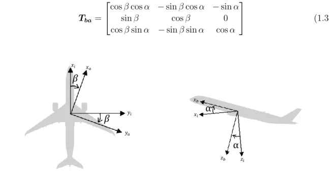
1.4 Geodetic and body reference frames . . . 24

1.5 Euler angles defining the orientation of the body frame (b) with respect to the geodetic frame (E). Intermediate axes (1, 2) are defined for the rotation sequence. . . 24

1.6 Angle of attack (α) and sideslip (β) defining the orientation of the aero-dynamic reference system (a) with respect to the body frame (b). Inter-mediate axes (i) are defined for the rotation sequence. . . 26

1.7 Global FEM model . . . 28

1.8 Condensed FEM model with structural reference frame . . . 28

2.1 Integration approach between nonlinear flight dynamics and linear aeroe-lastic equations of motion . . . 38

2.2 Illustration vertical gust effect and downwash on the aircraft . . . 40

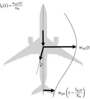
2.3 Illustration lateral gust effect and sidewash on the aircraft . . . 44

3.1 Gust profiles in time domain . . . 53

3.2 Gust profiles in frequency domain . . . 53

3.3 GAF in lift due to vertical gust . . . 54

3.4 GAF in pitch due to vertical gust . . . 55

3.5 Heave, pitch and vertical gust modes at a frequency close to zero (source:[17]) . 55 3.6 Comparison of GAF in lift due to heave motion, pitch rotation and vertical gust 55 3.7 Lift coefficient of fixed rigid A/C due to vertical gust (H=150ft) . . . 56

3.8 Pitching moment coefficient of fixed rigid A/C due to vertical gust (H=150ft) 56 3.9 GAF in lift due to vertical gust . . . 56

3.11 GAF in roll due to lateral gust . . . 57

3.12 GAF in yaw due to lateral gust . . . 58

3.13 Rolling moment coefficient of fixed rigid A/C due to lateral gust (H=150ft) 58

(10)

3.14 Yawing moment coefficient of fixed rigid A/C due to lateral gust (H=150ft) 58

3.17 Lift coefficient of fixed rigid A/C due to vertical gust (H=300ft) . . . 60

3.18 Pitching moment coefficient of fixed rigid A/C due to vertical gust (H=300ft) 60

3.31 Lift coefficient of quasi-steady flexible A/C due to vertical gust (H=300ft) 65

3.32 Pitching moment coefficient of quasi-steady flexible A/C due to vertical

gust (H=300ft) . . . 65

3.33 Lift coefficient of quasi-steady flexible A/C due to vertical gust (H=300ft) 65

gust (H=300ft) . . . 65

3.35 Rolling moment coefficient of quasi-steady flexible A/C due to lateral gust

(H=300ft) . . . 66

3.36 Yawing moment coefficient of quasi-steady flexible A/C due to lateral gust

(H=300ft) . . . 66

3.37 Rolling moment coefficient of quasi-steady flexible A/C due to lateral gust

(H=300ft) . . . 66

3.38 Yawing moment coefficient of quasi-steady flexible A/C due to lateral gust

(H=300ft) . . . 66

3.39 Lift coefficient of quasi-steady flexible A/C due to vertical gust (H=300ft)

for different CG . . . 67

gust (H=300ft) for different CG . . . 67

3.41 Illustration of the effect at different centre of gravity positions in vertical 68

3.42 Rolling moment coefficient of quasi-steady flexible A/C due to vertical gust

(H=300ft) for different CG . . . 68

3.43 Yawing moment coefficient of quasi-steady flexible A/C due to vertical

(11)

3.44 Illustration of the effect at different centre of gravity positions in lateral . 69

3.45 Illustration of the roll damping . . . 69

3.46 Rolling moment coefficient of free flying rigid A/C due to vertical gust

(H=300ft) for different wing dihedral . . . 70

3.47 Yawing moment coefficient of free flying rigid A/C due to vertical gust

(H=300ft) for different wing dihedral . . . 70

3.48 Illustration of the dihedral effect with and without static deformation . . 70

3.49 Lift coefficient of free flying rigid and quasi-steady flexible A/C due to

vertical gust (H=300ft) . . . 71

3.50 Pitching moment coefficient of free flying rigid and quasi-steady A/C due

to vertical gust (H=300ft) . . . 71

3.51 Rolling moment coefficient of free flying rigid and quasi-steady flexible

A/C due to lateral gust (H=300ft) . . . 71

3.52 Yawing moment coefficient of free flying rigid and quasi-steady A/C due

to lateral gust (H=300ft) . . . 71

3.53 Lift coefficient of free flexible A/C due to vertical gust (H=300ft) . . . . 72

3.54 Pitching moment coefficient of free flexible A/C due to vertical gust (H=300ft) 72

3.57 Low frequency modes which impact lift force and pitching moment coefficients

(Wing and fuselage bending and symmetric engine modes with amplification

factor) . . . 73

3.60 Rolling moment coefficient of free flexible A/C due to lateral gust (H=300ft) 74

3.61 Yawing moment coefficient of free flexible A/C due to lateral gust (H=300ft) 74

3.64 Low frequency modes which impact rolling and yawing moment coefficients

(Wing and fuselage antisymmetric bending and engine antisymmetric modes

with amplification factor) . . . 75

3.69 Lift coefficient of quasi-steady flexible A/C due to different vertical gust

profiles . . . 77

3.70 Pitching moment coefficient of quasi-steady flexible A/C due to different

(12)

3.71 Vertical load factor of quasi-steady flexible A/C due to different vertical

gust profiles . . . 78

3.72 Pitch angle of quasi-steady flexible A/C due to different vertical gust profiles 78

3.73 Lateral load factor of quasi-steady flexible A/C due to different lateral gust

profiles . . . 78

3.74 Roll angle of quasi-steady flexible A/C due to different lateral gust profiles 78

3.75 Roll rate of quasi-steady flexible A/C due to different vertical gust profile 79

3.76 Yaw rate of quasi-steady flexible A/C due to different vertical gust profile 79

3.87 Wing station at which the increment of pressure coefficient (∆Cp) is

cal-culated . . . 82

3.88 Increment of Cp distribution due to a low amplitude gust profile (scaled) with

respect to the steady condition at different time steps for a fixed rigid A/C

(M=0.836, h=27000ft) . . . 83

3.89 Increment of Cp distribution with respect to the steady condition at different

time steps for a fixed rigid A/C (M=0.5, h=0ft) . . . 83

time steps for a fixed rigid A/C (M=0.836, h=27000ft) . . . 84

3.93 Pressure distribution when the maximum amplitude of the gust disturbance

reaches the wing and zoom to the outer wing region where flow weakens . . . . 85

3.94 Lift force coefficient as a function of the steady angle of attack (M=0.836,

h=27000ft) . . . 85

3.95 Pressure distribution when the maximum amplitude of the gust disturbance

reaches the wing and zoom to the outer wing region where local stall appears . 86

(13)

time steps for a free flexible A/C (M=0.836, h=27000ft) . . . 89

3.103 Increment of Cp distribution due to a low amplitude gust profile (scaled) with respect to the steady condition at different time steps for a free flexible A/C (M=0.836, h=27000ft) . . . 89

3.105 Pitching moment coefficient of free flexible A/C due to vertical gust (H=150ft) 89 3.106 GAF in lift due to vertical gust for different Mach . . . 90

3.107 GAF in lift due to vertical gust for different Mach . . . 90

3.108 GAF in pitch due to vertical gust for different Mach . . . 91

4.1 PSD Von Karman turbulence spectrum . . . 94

4.2 Continuous wind turbulence in the time domain given by the Von Karman spectrum . . . 94

4.3 Pitch rate due to Von Karman turbulence spectrum (L=2500ft, σt=3) . 96 4.4 PSD pitch rate due to Von Karman turbulence spectrum (L=2500ft, σt=3) 96 4.5 Vertical load factor due to Von Karman turbulence spectrum (L=2500ft, σt=3) . . . 96

4.6 Yaw rate due to Von Karman turbulence spectrum (L=2500ft, σt=3) . . 97

4.7 PSD yaw rate due to Von Karman turbulence spectrum (L=2500ft, σt=3) 97 4.8 Roll rate due to Von Karman turbulence spectrum (L=2500ft, σt=3) . . . 97

4.9 PSD Von Karman turbulence spectrum . . . 98

4.10 Continuous wind turbulence in the time domain given by the Von Karman spectrum . . . 98

4.11 Pitch rate due to Von Karman turbulence spectrum (L=50ft, σt=3) . . . 99

4.12 Vertical load factor due to Von Karman turbulence spectrum (L=50ft, σt=3) . . . 99

4.13 Roll rate due to Von Karman turbulence spectrum (L=50ft, σt=3) . . . . 99

4.14 Yaw rate due to Von Karman turbulence spectrum (L=50ft, σt=3) . . . 99

4.15 PSD vertical measured turbulence spectrum . . . 100

4.16 Vertical measured turbulence in the time domain . . . 100

4.17 Pitch rate due to turbulence . . . 101

4.18 PSD pitch rate due to turbulence . . . 101

4.19 Vertical load factor at CG due to turbulence . . . 101

4.20 Yaw rate due to turbulence . . . 102

4.21 PSD yaw rate due to turbulence . . . 102

4.22 Illustration of gust angular speed induced by variations along the wingspan 103 4.23 Gust angular speed in roll and difference of vertical load factor between both wingtips . . . 104

(14)

4.24 Cross-power spectral density estimate between Pwind and measured roll

rate . . . 104

4.25 Cross-power spectral density estimate between Pwind and vertical turbu-lence measure . . . 105

4.26 Magnitude-squared coherence estimate between Pwind and vertical turbu-lence measure . . . 105

4.27 Cross-power spectral density estimate between Pwind and lateral turbu-lence measure . . . 105

4.28 Magnitude-squared coherence estimate between Pwind and lateral turbu-lence measure . . . 105

4.29 Roll rate due to turbulence . . . 106

4.30 PSD roll rate due to turbulence . . . 106

4.31 Yaw rate due to turbulence . . . 106

4.32 PSD yaw rate due to turbulence . . . 106

4.33 Vertical load factor at CG due to turbulence . . . 106

(15)

Abbreviations

A/C Aircraft

AIC Aerodynamic Influence Coefficient

CFD Computational Fluid Dynamics

CG Centre of Gravity

CSM Computational Structural Mechanics

DES Detached Eddy Simulation

DLM Doublet Lattice Method

DLR Deutsches Luft- und Raumfahrt Zentrum (German Aerospace Center) DVA Disturbance Velocity Approach

FEM Finite Element Method

FM Flight Mechanics

FRF Frequency Response Function GAF Generalized Aerodynamic Force GMRes Generalized Minimal Residual HTP Horizontal Tail Plane

LES Large Eddy Simulations

LFD Linearized Frequency Domain LIDAR Light Detection and Ranging

LU-SGS Lower-Upper Symmetric-Gauss-Seidel MAC Mean Aerodynamic Chord

ODE Ordinary Differential Equation PDEs Partial Differential Equations

PSD Power Spectral Density

RANS Reynolds Averaged Navier Stokes RBF Radial Basis Function

RFA Rational Function Approximation ROM Reduced Order Model

VTP Vertical Tail Plane VLM Vortex Lattice Method

(16)

Greek Symbols

α Angle of attack

αG Angle of attack due to a vertical gust or turbulence disturbance

β Sideslip

βG Sideslip due to a lateral gust or turbulence disturbance

γ Heat capacity ratio

δ Finite-difference step size

∆ Increment

ε Downwash

θ Pitch attitude angle

Θ Euler angles

λ Gust wavelength

ν Mesh cell volumes in a matrix

ρ Airflow density

σ Sidewash

σt Root-mean-square turbulence velocity

σy Root-mean-square value of the aircraft response to turbulence

τ Viscous stress tensor

τG Time constant of a first order filter associated with the gust-induced effect

τn/w Time delay from the aircraft nose section to the aerodynamic centre of the wing

τn/H Time delay from the aircraft nose section to the HTP

τw/H Time delay from the aerodynamic centre of the wing to the HTP

τw/V Time delay from the aerodynamic centre of the wing to the VTP

ϕ Gust phase shift

φ Roll attitude angle

φp Total velocity potential

φk Power spectral density of the Von Karman turbulence velocity profile

φv Perturbation velocity potential

φy Power spectral density of the aircraft response to turbulence

φxz Cross power spectral density between measures x and z

φ Modal matrix

ψ Heading angle

Ψ Acceleration potential

ω Angular frequency

Ω Spatial frequency

Ωb Angular velocity (body axes)

Latin Symbols

a∞ Freestream speed of sound

B Damping matrix

(17)

Cl Rolling moment coefficient

Clβ Rolling moment gradient due to a sideslip variation

C_{l ˙}_β

G Dynamic rolling moment gradient due to lateral atmospheric disturbance

Clp Rolling moment gradient due to a roll rate variation

Clpwind Rolling moment gradient due to gust or turbulence variation along wingspan

Cm Pitching moment coefficient

Cmα Pitching moment gradient due to an angle of attack variation

Cm ˙αG Dynamic pitching moment gradient due to vertical atmospheric disturbance

Cn Yawing moment coefficient

Cnβ Yawing moment gradient due to a sideslip variation

C_{n ˙}_β

G Dynamic yawing moment gradient due to lateral atmospheric disturbance

Cp Pressure coefficient

Cx Drag coefficient

Cy Side-force coefficient

Cyβ Side-force gradient due to a sideslip variation

C_{y ˙}_β

G Dynamic side-force gradient due to lateral atmospheric disturbance

Cz Lift force coefficient

Czα Lift force gradient due to an angle of attack variation

Cz ˙αG Dynamic lift force gradient due to vertical atmospheric disturbance

Cxz Coherence between measures x and z

D Transformation matrix relating body and Euler angular rates

d Viscous fluxes

di Delay coefficients of the rational function approximation

E Energy per unit volume

Fb External (aerodynamic) forces (body axes)

Fg Forces applied to the structural grid

Fh Modal forces

Fi, Fhhi, FhGi Coefficients of the rational function approximation

f Inviscid fluxes

f Frequency

GE Gravitational vector (geodetic axes)

Ggj Spline to project forces from aerodynamic to structural grid

g Gravity

H Half of the gust wavelength

Hy Aircraft frequency response in turbulence

h Altitude

I Identity matrix

Jb Total inertia tensor

j Complex imaginary unit (√−1)

(18)

k Reduced frequency

L Turbulence scale wavelength

LE Position vector of aircraft centre of gravity in geodetic reference frame

lref Reference chord length

ln/w Distance from the aircraft nose section to the aerodynamic centre of the wing

ln/H Distance from the aircraft nose section to the HTP

lw/H Distance from the aerodynamic centre of the wing to the HTP

lw/V Distance from the aerodynamic centre of the wing to the VTP

M Mass matrix

M Mach number

Mb External (aerodynamic) moments (body axes)

m Total aircraft mass

Nd Number of delay coefficients of the rational function approximaton

Ny Lateral load factor

Nz Vertical load factor

P Pressure

Pwind Gust angular speed (roll)

p Roll rate

Q Aerodynamic influence coefficient

Qhh Motion-induced generalized aerodynamic force

QhG Gust-induced generalized aerodynamic force

q Power exchanged by conduction

q Pitch rate

¯

q Dynamic pressure

R Non-linear fluid residual

r Yaw rate

rCG−25% Position vector between aircraft CG and origin of aerodynamic reference frame

s Laplace variable

Sref Reference area (wing surface)

SH HTP surface

SV VTP surface

TbE Transformation matrix from geodetic frame to body axis

Tba Transformation matrix from aerodynamic frame to body axis

t Time

U Model inputs (state-space model)

ub x-component of velocity of aircraft centre of gravity in body axes

uh Generalized coordinate

ue Flexible generalized displacement

ue0 Quasi-static flexible generalized displacement

(19)

V∞ Freestream true airspeed

VH True airspeed at HTP aerodynamic centre

VV True airspeed at VTP aerodynamic centre

Vb Translational velocity (body axes)

v Flow velocity

vb y-component of velocity of aircraft centre of gravity in body axes

wb z-component of velocity of aircraft centre of gravity in body axes

wG Gust or turbulence disturbance

wyG Lateral component of gust or turbulence disturbance

wzG Vertical component of gust or turbulence disturbance

X Aircraft states (state-space model)

x Spatial position

xr Rigid aircraft states (state-space model)

xe Flexible aircraft states (state-space model)

xL States associated with delays due to gust or turbulence inputs (state-space model)

xcg x-component of aircraft centre of gravity

xg Structural displacement

Y Model outputs (state-space model)

yf Conservative flow variable

Operators

× Vector cross product

()T _Transpose ()−1 Inverse ∂() ∂() Partial derivative d() d() Total derivative ˙ () Time derivative (∂()_∂t) ∇ · () Divergence ∇() Gradient () Complex conjugate k()k Vector norm |()| Absolute value Subscripts 0 Initial value

a Aerodynamic reference frame

b Body reference frame

E Geodetic reference frame

e Elastic degrees of freedom

f Fluid

(20)

g Structural coordinates H HTP h Modal coordinates j Aerodynamic grid/coordinates L Lag states n Aircraft nose

r Rigid degrees of freedom

s Steady state

V VTP

w Wing

Superscripts

cs Control surface deflection effect

f lex Dynamic flexibility effect

gust Gust-induced effect

QS Quasi-steady, quasi-static

u Motion-induced effect

(21)

Context

Gust and atmospheric turbulence, which can be seen as sudden movement of the air around the aircraft, have been considered from the earliest days of aviation in order to ensure successful flights [1, 2]. These changes in air velocity modify the effective incidence seen by the body surfaces, creating aerodynamic forces and moments which cause a dynamic response of the aircraft. This response may involve different rigid as well as flexible motion according to the atmospheric disturbance, creating internal loads in addition to trajectory and attitude variations of the vehicle that need to be considered in different aircraft analysis and design tasks.

The simulation of the aircraft response in such cases is a multidisciplinary problem rel-evant for different applications. Aircraft design and certification require gust load analysis in order to ensure that the airframe is able to withstand the internal loads due to gust and turbulence [3, 4]. This defines the structural sizing and as a result, the aircraft weight. Uncertainties related to the model used for the loads calculation are translated into design margins.

The effect of gust and turbulence on aircraft flight dynamics is also of interest to evaluate the aircraft response and flight control laws in realistic atmospheric disturbances. Flight tests analysis is an important part of this kind of analysis. Possible flight control law tuning from the initial design also relies on flight test. Modelling improvements before the flight test phase could enable cost and lead time reduction. Enhanced simulation means could also allow the possibility to propose strategies to attenuate the gust and turbulence effects on the aircraft response.

For different purposes, gust loads as well as flight dynamic analysis require accurate means able to predict the aircraft response in these conditions in early design phases. Within this context, understanding and modelling the relevant physics involved leading to accurate simulations is essential.

Gust loads and flight dynamics applications require low computing times as several flight conditions and aircraft parameters are evaluated. Different aerodynamic simulation

(22)

approaches with different levels of fidelity can be used to generate computationally efficient unsteady aerodynamic models used to capture the gust and turbulence induced effects.

Appart from considering the atmospheric contribution, the aircraft rigid and flexible motion create additional aerodynamic forces and moments. An example of the simulation of the aircraft response due to a vertical gust is shown in figure 1. The aircraft before the gust encounter is also included. The wing flexible deformation modifies the angle of attack in addition to the variation created by the external gust profile, changing the lift force and affecting the overall aircraft response. These effects are also of importance when simulating the aircraft response in these cases.

Figure 1: Illustration of the simulation of the aircraft response due to a vertical gust The aircraft response can be simulated with different approaches covering the needs for specific applications. Models of different nature are traditionally used for flight dynamics and gust loads calculations.

Flight dynamics analysis are based on nonlinear time domain simulations with a cor-rected aerodynamic model to account for flexible deformation, assuming that the structure is in static equilibrium [5]. Dynamic effects due to rapid changes in rigid motion, flexible deformation or external aerodynamics are not taken into account and perturbations have an instantaneous effect on the aerodynamic forces. This assumption is referred to as quasi-steady aerodynamics and is sufficient to capture the main effects of slow manoeuvres of current aircraft passenger configurations. Nonlinear aerodynamic effects such as stalls as well as compressible effects appearing at high Mach numbers are included in the model. As the interest in flight dynamics is the study of the global aircraft response, aerodynamic forces and moments can be calculated though global aerodynamic coefficients with respect to a reference point, such as the aerodynamic centre. Different local and component effects are superposed and considered with respect to the reference point. The gust and turbu-lence profiles affect locally the aircraft parts at different times, due to the atmospheric disturbance propagation at a certain speed all along the vehicle.

Gust loads require the use of aeroelastic models to calculate the dynamic response [2]. This approach combine a structural model and a linear unsteady aerodynamics model usu-ally expressed in the frequency domain. The aerodynamic forces are distributed all along the aircraft enabling local analysis for the structural sizing of the different components.

(23)

Dynamic effects due to motion and external disturbances are taken into account. Cor-rections are required to extend the range of validity of the linear aerodynamic model, in particular at transonic speeds close to cruise, where aerodynamic nonlinear effects appear. Integration of methods and data from both approaches are of interest for multidis-ciplinary analysis, consistency between domains and overcome some of the limitations of each strategy. These kind of integration approaches are explored and proposed in this work in the framework of the simulation of the flexible aircraft response to gust and turbulence for flight dynamics investigations. The overall aircraft response also affects the calculated gust loads used to size the structure. Improved means to predict the global aircraft re-sponse could lead to more accurate gust loads. Local analysis which are not considered in the present work, are required to capture the level of loads in all the different structural components (shear force, bending and torsional moments).

Previous work

Extensive research has been previously focused on the simulation and modelling of the gust and turbulence effects on the aircraft response as well as the development of integrated flight dynamics and aeroelastic models. This section includes previous work on both topics contributing to the possibility to simulate the free flying flexible aircraft response due to gust and turbulence.

Gust and Atmospheric Turbulence Effects

Many possibilities for modelling unsteady aerodynamic effects are proposed in the litera-ture. The traditional approach used during the last decades for gust loads analysis consist in calculating the gust and turbulence induced unsteady aerodynamic forces through po-tential flow equations over a range of frequencies with panel methods such as the Doublet Lattice Method (DLM), which captures unsteady effects without taking into account the steady state condition [6]. Corrections with wind tunnel and steady Computational Fluid Dynamics (CFD) data have been used to overcome limitations of panel methods, in par-ticular in the transonic regime [7].

Other possibilities in early design phases can be considered as studied by Kier [8]. Different simulation methods with different modelling assumptions are compared by pre-dicting the estimated gust loads in the time domain. Predictions from DLM are compared with quasi-steady Vortex Lattice Method (VLM), the steady strip theory and the unsteady strip theory with the Wagner and Küssner indicial functions [2]. The effect of gust propa-gation as well as the lags associated with the unsteady aerodynamic response are observed when evaluating the differences between the approaches. Recommendations are provided for preliminary gust loads design objectives.

(24)

Some advantages of a 3D panel method in comparison to DLM are shown by Kier [9] for lateral gust loads and flight dynamic analysis in early design phases. In particular, the 3D panel method is able to capture relevant flight dynamic effects such as the roll-yaw coupling which affects the flight mechanical modes like the dutch roll. These effects are not taken into account by DLM as in plane aerodynamic effects are not considered. DLM requires corrections to include some of the neglected physics. A 3D panel method is also used by Staveren [10] to identify gust stability derivatives to simulate one-dimensional (1D) and two-dimensional (2D) turbulence inputs. The method is used to calculate both the quasi-steady and unsteady stability derivatives using harmonic analysis from the aircraft frequency response functions. The identified gust derivatives are then dependent of the gust scale length and aircraft mass. The approach is compared with some analytical single-point and multi-point aircraft models presented in [11].

Some of the modelling limitations of panel methods have been pointed out by using higher fidelity simulation means, such as CFD, in particular at transonic conditions. High fidelity methods can be used to correct panel methods or to directly calculate the gust induced effect. The application of nonlinear CFD in the time domain to simulate the aircraft response of a flexible aircraft due to gust encounters is compared with classical DLM by Reimer et al. [12]. The multidisciplinary coupling framework of a CFD based approach is presented to account for flight dynamics and structural deformation. However, gust loads analysis as well as flight dynamics investigations require the simulation of a large number of cases with several parameter variations. The use of nonlinear CFD for unsteady purposes in the time domain involves large computation times.

Instead of solving nonlinear CFD directly in the time domain, recent developments have shown the possibility to obtain accurate aerodynamic predictions in the transonic regime with a low computational cost through linearized frequency-domain (LFD) methods. This approach, also known as time-linearized or linear harmonic small disturbance method, offer a large computational efficiency improvement while maintaining the accuracy of non-linear CFD. The governing equations are linearized around a non-linear steady state assuming low amplitude harmonic disturbances. This allows retaining the aerodynamic steady non-linearities such as shock waves as well as shock-induced local separation. The approach is proposed and validated by Thormann and Widhalm [13] in order to predict forced-motion unsteady aerodynamic effects and determine the flutter boundaries at high Mach numbers. Widhalm et al. [14] also propose a linearized approach as an appropriate strategy to cover wide parameter variations in a reasonable computational cost to extract dynamic stability derivatives. Both subsonic and transonic conditions are evaluated and results are validated against experimental data as well as time accurate unsteady CFD simulations.

The extension of the linearized CFD approach to solve unsteady aerodynamic effects due to gust encounters is presented by Bekemeyer and Timme [15]. Aerodynamic responses of an airfoil due to different gust profiles are obtained by superposing several frequency domain results at subsonic and transonic flight conditions. The maturity of the method is

(25)

demonstrated by Bekemeyer et al. [16] by efficiently computing the aerodynamic response to gust for a three dimensional relevant industrial case. Responses in the time domain are obtained by using a complex-valued weighting function in combination with the su-perposition of responses at discrete frequencies. Global lift as well as surface pressure distributions are calculated for a large civil aircraft and validated against nonlinear CFD in the time domain. The progress achieved in linearized CFD allowed the possibility to use unsteady CFD in an industrial context for gust loads calculations as shown by Weigold et al. [17]. This enables the possibility to avoid or minimise the adjustments required for panel methods. Advantages of using linearized CFD in the design of a gust loads alleviation at transonic conditions are also shown by Bekemeyer et al. [18].

The gust low amplitude assumption is not always respected and dynamic non linear effects that are not captured by linearized CFD may appear. Corrections to account for unsteady nonlinear effects at low frequencies have been recently investigated by Thormann and Timme [19]. The harmonic balance method is employed by using a small number of harmonics to correct the low frequency range while using the linearized frequency do-main CFD at higher frequencies. Different gust encounters are considered to calculate the aerodynamic and aeroelastic response of an airfoil at transonic conditions.

Other strategies have been investigated to better account for nonlinear unsteady aero-dynamic effects through the form of a CFD-based Reduced Order Model (ROM). This topic has been widely investigated in order to provide modelling strategies in the nonlinear aerodynamic region for many applications. An overview of nonlinear ROM applied to aero-dynamics and aeroelasticity is given by Ripepi [20]. Some approaches have been proposed to deal with the specific problem of the nonlinear aerodynamic response of an aircraft to gust and turbulence. Quero et al. [21] present a ROM in the frequency domain based on the identification of Volterra kernels by continuous time impulses to predict the nonlinear aerodynamic response to gust and turbulence encounters. Bekemeyer et al. [22] propose another unsteady nonlinear ROM for gust load predictions based on least-squares residual minimization of the full order model projected in a reduced space. More accurate predic-tions are shown with respect to a linearized CFD approach once unsteady aerodynamic nonlinearities appear.

Unsteady aerodynamic forces calculated by linearized CFD or DLM are expressed in the frequency domain. Forces can be obtained in the time domain by different approaches. One of the possibilities consists in fitting the frequency data with rational functions in the time domain through the Rational Function Approximation (RFA) method proposed by Roger [23]. The method captures the unsteady effects in the time domain by introducing additional aerodynamic states, also referred to as lag states. This method has been widely used for various aeroservoelastic applications. Different forms have been proposed in order to keep the minimum number of additional lag states, such as the minimum state-method developed by Karpel [24].

(26)

Googin [25] proposes an aeroservoelastic method for manoeuvre and gust loads calcu-lations in the time domain. An alternative RFA approach is applied, by adding explicit delays to the classic form proposed by Roger [23]. These delays can be associated with different parts of the aircraft, such as the nose, the wing and the tail. Compared to the classic RFA approximation, the RFA with explicit delays requires less additional lag states and is found to be more accurate at higher frequencies and predicting local gust loads in the rear part of the aircraft, where gust propagation effects are important. Weighting factors are proposed to correct the RFA to account for experimental data or quasi-steady aerodynamic nonlinearities.

Different frequency and time domain approaches to simulate the dynamic aircraft re-sponse to atmospheric gust excitations are presented by Karpel et al. [26]. The possibility to divide the aircraft in zones is also proposed to increase the accuracy of the RFA. These time delays can also be approximated by delay filters of different order in cases the use of explicit delays for each zone is not possible.

Kier and Looye [27] deal with the problematic of approximating the phase shift associ-ated with the gust propagation effect. In the frequency domain, the time lags associassoci-ated with the gust effect all along the aircraft are expressed as phase shifts with an exponential function, which can be difficult to capture in the time domain. Instead of approximating the gust column in the time domain, the proposed approach consists of expressing the gust downwash as a function of time thanks to the relative location between the aircraft and the gust through the propagation speed. A RFA with distributed coefficients over the aircraft is calculated in order to evaluate the aerodynamic effect of the downwash associated with the gust velocity as a function of time. The same approach, dividing the aircraft in five sections, is applied to the design of a gust load alleviation function by Giesseler at al. [28]. Quero et al. [29] proposed an alternative to the classical Roger approximation [23] for cases in which gust-induced forces are required at higher frequencies, such as for gust loads analysis in the time domain. The approach is based on tangential interpolation and provides a minimal order approximation, avoiding any selection of lag states.

Integrated Aircraft Model

Once the aerodynamic forces and moments due to the atmospheric disturbance are calcu-lated, the equations of motion are used to predict the aircraft response to these forces. The integration of flight dynamics and aeroelastic equations of motion offers the possibility to account for both rigid and flexible motion. The definition and formulation of these kind of integrated approaches have been addressed by several authors.

A derivation of these equations of motion from first principles using the Lagrange’s equations and the principle of virtual work was proposed by Waszak and Schmidt [30, 31]. Aerodynamic generalized forces are obtained through strip theory in a closed form integral

(27)

expression. The reference axes are appropriately chosen in order to minimise the inertial coupling between rigid and flexible motion, through the concept of mean axes reference frame. The use of free vibration modes to express the flexible motion automatically fulfils the practical mean axes constraints of the reference frame minimising the intertial cou-pling. Additional inertial coupling terms are neglected. The nonlinear equations of motion of the integrated model describe the aircraft motion relative to body axes and the elastic deformation of the airframe relative to this reference frame. These differential equations for flight mechanics and aeroelastic motion are only coupled through the external aerody-namic forces. The same equations are obtained by Etkin [5] when adding the aerodyaerody-namic coupling terms due to the flexible degrees of freedom to the flight dynamics equations of motion.

The inertial coupling effects in the equations of motion of a free flying flexible aircraft are studied by Buttrill et al. [32]. The formulations and assumptions of the integrated equations of motion from Waszak [30, 31] and Buttrill [32] are compared in [33], providing possible simplifications as well as recommendations concerning the importance of the iner-tial coupling terms. Ineriner-tial coupling between the rigid and flexible degrees of freedom is taken into account in the derivation of the equations of motion done by Reschke [34] for a generic current passenger aircraft configuration. The effects on the flight dynamic states of considering an inertially coupled formulation are found to be small. An important effect of the inertial coupling is detected in structural components with large concentrated masses, such as the engines. The influence of inertial coupling on loads is found to be relevant at flight conditions with high angular rates or accelerations.

Various simulation environments are proposed to implement different integration strate-gies between models. One of the possibilities is VarLoads presented by Hofstee et al. [35] proposed for specific investigations from preliminary design to the analysis of in-flight events. The modular software structure of the environment allows the possibility to im-plement different models from various disciplines. The nonlinear equations of motion de-veloped by Waszak and Schmidt [31] are implemented.

Apart from the equations of motion, an integrated approach between flight dynamics and aeroelastic responses needs to address the combination between different aerodynamic models dealing with different assumptions and data sources.

Rigid nonlinear quasi-steady aerodynamics are combined with an unsteady aerodynamic model from DLM in the work done by Gupta et al. [36]. A padé approximation similar to the RFA from Roger [23] is employed to express the unsteady aerodynamic forces in the time domain. The rigid quasi-steady contribution is removed from the unsteady forces.

When the quasi-steady aerodynamics model is corrected to account for quasi-static flexible effects, some aspects need to be considered when integrating both aerodynamic models. The work presented by Winther et al. [37] deals with this problematic and proposes a method to combine dynamic effects from the aeroelastic equations of motion with the

(28)

nonlinear quasi-steady flexible equations used for flight dynamics analysis. It is assumed that the rigid body dynamics of the residualized linear aeroelastic model are equivalent to the linearized flight dynamics model including quasi-static flexible corrections. The integrated model aims for real-time simulations and recommendations are given to keep low computational times. The approach, referred to as Residualized Model, is extended in the work proposed by Looye [38], providing the possibility to use aeroelastic models with unsteady aerodynamic lag states.

Another strategy presented by König and Schuler [39] proposes adding the states of a linearized or nonlinear flight dynamics equations of motion in an aeroelastic model. A modal analysis is employed to decouple rigid and flexible motion. The rigid body modes of the aeroelastic model need to be identified and are replaced by the states of the linearized or nonlinear flight dynamics equations of motion. It is assumed that the flight dynamic states are equivalent to a linear combination of rigid body modes of the aeroelastic model. The strategy is applied in the design of a controller through multi-objective parameter op-timization for flight control, loads reduction and structural mode control. The integration of a linearized flight dynamics and aeroelastic model without coupling terms is also applied to different multi-objective control design techniques in the work presented by Puyou [40]. The work done by Reschke and Looye [41] compares the König and Schuler approach [39] and the Residualized Model method proposed by Looye [38]. The different assumptions, some pre-processing and implementation details as well as advantages of each approach are included. Both methods are based on the idea of keeping the flight dynamics model unchanged. Results obtained as well as computational times are found to be similar for both approaches. Recommendations to choose between them are based on the simulation environment.

Another possibility to integrate nonlinear quasi-steady aerodynamics with linear un-steady aerodynamics is proposed by Kier and Looye [27]. A set of nonlinear equations of motion as developed in [30, 31] are used. The quasi-steady aerodynamic effects are mod-elled through VLM. Unsteady aerodynamics are considered through a RFA of results from DLM according to Roger’s method [23] for time domain simulations. Instead of projecting the aerodynamic forces to modal coordinates (generalized forces) before the approximation, the RFA is done in physical coordinates directly in the aerodynamic grid. This enables a clear separation between quasi-steady and unsteady terms which may come from different models. This has also the advantage that the approximation is only dependent on the Mach number and is not tied to a mass case like the modal unsteady aerodynamic forces. Different applications can be found in literature. Teufel et al. [42] applies an integrated flight mechanics and aeroelastic model to predict the dynamic response of a large passenger aircraft to multidimensional gusts. These integration approaches have also been applied both for loads analysis [27] as well as for specific flight control law design strategies [28, 38].

(29)

Objectives

The main goal of the PhD is to propose a modelling approach able to capture relevant aerodynamic effects due to gust and turbulence in the frequency range of interest for flight dynamics investigations. The strategy is intended to capture relevant physics when simulating the gust and turbulence effect on flight dynamics, providing more accuracy in the predictions and minimising the increase of computational cost.

The topic requires an understanding of the main physics involved in order to propose appropriate models to capture the relevant effects. A strategy to generate the required data for the model, covering different parameters in a reasonable computation time, is also needed within an industrial context. Validation means and recommendations on the application of the proposed models are also necessary. One of the challenges when dealing with experimental data from flight test is the level of uncertainty of the gust or turbulence inputs encountered in flight.

Enhanced simulation means to capture the aircraft response in such conditions and keeping consistency between gust loads as well as flight dynamics analysis is of interest for multidisciplinary analysis in early design phases, which is essential for future aircraft developments. Specific aspects concerning flight dynamics analysis need to be addressed, such as the possibility to provide simulation means that could be integrated in the existing real-time simulation environments in the form of aerodynamic stability derivatives. The possibility to account for the effect of flight control laws in the time domain is also required for meaningful flight dynamics investigations.

Outline

In this PhD, and based on some of the previous work concerning the topic, an integrated approach including gust and turbulence induced effects is formulated and applied to sim-ulate the free flying flexible aircraft response due to different atmospheric disturbances.

In part I, the theoretical aspects of different simulation methods and models are detailed and proposed in order to predict the aircraft dynamic response due to gust and turbulence. The first chapter presents the aerodynamic formulation from higher to lower fidelity methods with its assumptions. The unsteady aerodynamic data is generated with CFD through its linearized form to cover a wide variation of parameters, such as the Mach number, keeping a reasonable computational time and avoiding corrections as the ones required to overcome the neglected physics of DLM. Nonlinear CFD in the time domain is also considered to validate the modelling approach and quantify the effect of possible aerodynamic nonlinearities in the global aircraft response. The remaining sections of this chapter deal with the means to predict the flight dynamics and aeroelastic response. The

(30)

equations of motion and aerodynamic models are described for each approach and details concerning the different modelling strategies are given.

The second chapter describes the integration framework to combine flight dynamics and aeroelastic models as well as how the gust-induced and dynamic flexible effects are considered. Some strategies to reduce the number of additional aerodynamic states, associ-ated with the gust-induced effect, are shown. As flight dynamics investigations are focused on the low frequency range, accurate predictions can be obtained by keeping a low num-ber of additional aerodynamic states in a rational function approximation. The analytical derivation of gust aerodynamic derivative coefficients for both vertical and lateral analysis is included as a possible mean to estimate the effect. Considering inertial coupling between rigid and flexible motion can provide more accuracy for specific load calculations but the effect on flight dynamics of current passenger aircraft configurations can be neglected. In this work, the external coupling through the aerodynamic forces is considered. Motion-induced unsteady aerodynamics from the flexible response are taken into account to assess the impact of dynamic flexibility on aircraft flight dynamics for current passenger aircraft configurations. Different forms of the residualized model approach are presented in order to account for the dynamic flexible effect.

In part II, the integrated approach is applied to simulate the aircraft response to gust and atmospheric turbulence. The theoretical inputs are assumed to be known and taken from the certification requirements [3]. Turbulence measured in flight is also considered as input for the simulation. Assumptions and uncertainties related to this measure are important and need to be taken into account for appropriate analysis. The analysis is done for both vertical and lateral atmospheric disturbances with different approaches and modelling assumptions detailed in the previous section. As the work is focused on the effect of gust and turbulence on flight dynamics, the variables of interest predicted and analysed through the different modelling strategies are aerodynamic global coefficients or quantities such as load factors at the centre of gravity as well as angular rates (roll, pitch, yaw). A generic current passenger aircraft configuration is used to evaluate the different simulation methods.

The third chapter focuses on the aircraft response to theoretical gust profiles at different flight conditions. Once the model is created and validated, some of the relevant physics as well as modelling assumptions are assessed. The predicted response to gust at transonic conditions is also evaluated in order to quantify the effect of possible shock motion or local stalls on the global response.

The fourth chapter focuses on the application of the approach to simulate the aircraft response due to theoretical as well as realistic atmospheric turbulence. Flight test measures are used to compare with simulation results. The effect of turbulence variations along the wingspan is discussed at the end of the chapter.

(31)

Theory

(32)

(33)

Simulation and Modelling of Aircraft

Dynamic Response

In this chapter, various aerodynamic formulations with different modelling assumptions are presented. The equations of motion used to calculate the aircraft response as well as the form of the models providing the aerodynamic forces and moments are detailed. The described approaches cover both flight dynamics and aeroelastic responses.

1.1 Aerodynamic Formulation

Aerodynamics simulation and modelling is an extensive domain. Different strategies can be applied covering the needs of specific applications. Simulation means from higher to lower fidelity with its underlying assumptions and modelling strategies are shown in this section. From the Navier-Stokes equations to solve the aerodynamic problem in the time domain, to the linearisation of the equations to solve it in the frequency domain as well as the traditional potential methods used for unsteady aerodynamic computations. The predicted aerodynamics from simulation means can be adjusted with experimental data such as wind tunnel or flight tests in order to extend the validity of the model within the flight envelope.

1.1.1 Reynolds Averaged Navier Stokes (RANS) Equations

The Navier-Stokes equations is the common approach used to capture the flow phenomena around the aircraft. The equations force the conservation of mass, energy and momentum by imposing the continuity equation, Newton’s second law of motion and the first law of thermodynamics. Additional empirical relations to define the fluid properties such as viscosity and thermal conductivity as well as a constitutive law are added to the system

(34)

of equations. Even if an important progress has been recently done in terms of computa-tional ressources, the Navier-Stokes equations are not suitable when dealing with relevant industrial problems. The adopted solution consists of using the Reynolds Averaged Navier Stokes (RANS) equations, in which the characteristic turbulent flow variations are aver-aged and a turbulence model is used to approximate the additional turbulent variations. The flow variables are then expressed as a time-average and a turbulent variation around the average condition.

According to the formulation employed by Ripepi and Quero [20, 43], the governing equations for a compressible, viscous and conductive fluid with constant properties in conservative form are:

∂yf

∂t + ∇ · f(yf) = ∇ · d(yf) (1.1)

Being yf the conservative flow variable vector which depends both on the spatial

po-sition (x) and time (t), the inviscid fluxes f and viscous fluxes d, defined respectively as: yf =   ρ ρv E   f =   ρv ρv × v + P I v(E + P )   d =   0 τ τ · v + q  

With ρ(x, t) being the density, v(x, t) the flow velocity, E the energy per unit volume, P (x, t) the pressure, τ (x, t) the viscous stress tensor, q(x, t) the power exchanged by conduction and I the identity matrix. The state equation for the pressure as well as the constitutive equations for the viscous stress tensor and the power exchanged by conduction lead to the closure of the problem. The resulting nonlinear Partial Differential Equations (PDEs) is solved by specifying the boundary and initial conditions of the problem.

These equations are averaged in time leading to the Reynolds Averaged Navier-Stokes (RANS) equations. This overcomes the high computational cost of the direct solution of the Navier-Stokes equations. Additional details about the formulation can be found in [44]. Increased accuracy can be achieved through alternative approaches such as the De-tached Eddy Simulation (DES) which combines RANS equations near wall regions and Large Eddy Simulations (LES) [45], the direct simulation of the rest of the flow.

(35)

In this study, steady and unsteady RANS equations have been solved by the use of the Computational Fluid Dynamics (CFD) code TAU from the DLR. Finite volume dis-cretization is employed on deformable unstructured meshes. This code has been applied and validated extensively in research and industry for both steady and unsteady problems [46].

The turbulence model used in all the simulations presented in this work is the Spalart-Allmaras model [47]. Steady solutions are obtained using the backward Euler implicit scheme with Lower-Upper Symmetric Gauss-Seidel (LU-SGS) iterations. Convergence is accelerated through a 2v multigrid scheme [48].

For the unsteady solution, the equations are integrated in time with the second order backward difference operator using a dual time stepping [48]. For subsonic problems, time step size is set to 0.004s with 100 inner iterations per time step. For transonic conditions, the time step size is set to 0.002s with 150 inner iterations per time step based on a similar configuration [49].

The method used to impose the atmospheric disturbances is the so called Disturbance Velocity Approach (DVA) (also known as Field Velocity Approach) [50]. The gust effect is added as a velocity term in the governing equations and prescribed in the mesh with no additional deformation of the grid required.

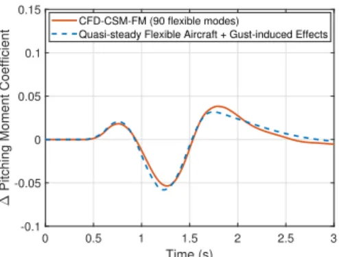
The resolution of the RANS equations in the time domain through CFD simulations can be applied for a detailed analysis of the relevant physics to quantify aerodynamic nonlinear effects in specific flight conditions [49]. In this case, these simulations are used for the validation of the model-based approach. The effect of possible aerodynamic nonlinearities is also analysed. In particular, when flying at high Mach numbers in transonic conditions, where shock motions or local stalls may appear due to gust and turbulence induced effects. The CFD solver can also be coupled with a computational structural mechanics (CSM) and flight mechanics (FM) solver in order to deform the mesh according to the structural deformation and rigid body response of the aircraft respectively. The framework FlowSim-ulator is used to handle the coupling, the different sets of data and simulations [51]. Details about the unsteady aerodynamic solution in the time domain have been previously pro-vided. Structural deformations are represented using a modal approach. The aerodynamic forces are projected to the different modes before calculating the aircraft response due to theses forces. The structural equations are solved through a Newmark time integration scheme [52]. Rigid body and flexible motion calculated through the equations of motion presented in the next sections of this chapter are interpolated into the CFD surface mesh. The appropriate mesh deformation to account for the aircraft rigid and flexible motion is calculated and applied using the radial basis function method (RBF). Further details on the deformation technique can be found in [53] and [54]. Appart from the 6 rigid body modes, 90 flexible modes are retained. A similar coupling approach can be found in [55].

(36)

unstructured mesh with 11.4 million points is used for a similar configuration as the one presented in [12]. The surface mesh is shown in figure 1.1.

Figure 1.1: CFD surface mesh

1.1.2 Linearized Reynolds Averaged Navier Stokes (RANS)

Equa-tions

The previous detailed RANS equations can be linearized around a nonlinear steady state condition. The formulation is presented according to Bekemeyer [56]. Applying a finite-volume discretisation of the governing equations, for a fixed flight condition, the ordinary differential equation (ODE) in semi-discrete form can be expressed as:

∂νyf

∂t = R(yf, x,x, w˙ G) (1.2)

with x and x being the change in mesh coordinates and their velocities respectively, w˙ G

being the gust disturbances which are accounted for through mesh velocities x. The term˙

R corresponds to the non-linear fluid residual of the unknowns of the problem and ν contains the cell volumes in a matrix.

An increment between the conservative flow variable and the steady state solution can be defined:

∆yf = yf − yf s (1.3)

Similarly, for gust disturbances ∆wG = wG − wGs, mesh coordinates ∆x = x − xs