an author's
https://oatao.univ-toulouse.fr/27067
https://doi.org/10.1016/j.ijplas.2020.102777
Ruiz De Sotto, Miguel and Longère, Patrice and Doquet, Véronique and Papasidero, Jessica A constitutive model for
a rate and temperature-dependent, plastically anisotropic titanium alloy. (2020) International Journal of Plasticity,
134. 102777. ISSN 0749-6419
A constitutive model for a rate and temperature-dependent,
plastically anisotropic titanium alloy
Miguel Ruiz de Sotto
a,b,c, Patrice Long�ere
a,*, V�eronique Doquet
b,
Jessica Papasidero
caICA, Universit�e de Toulouse, ISAE-SUPAERO, MINES ALBI, UPS, INSA, CNRS, 31000, Toulouse, France bLaboratoire de M�ecanique des Solides, CNRS UMR 7649, Ecole Polytechnique, 91128, Palaiseau, France cSafran Aircraft Engines, Rond Point Ren�e Ravaud, 77550, R�eau, France
Keywords: Titanium alloy Plastic anisotropy Dynamic plasticity Complex loading Numerical simulation MSC: 00-01 99-00 A B S T R A C T
Aircraft engine fan blades are notably designed to withstand impact loading involving large deformation, high strain rate, non-proportional loading paths and self-heating. Due to their high strength-to-weight ratio and good toughness, Ti–6Al–4V titanium alloys are promising candidates for the blades leading edge. An extensive experimental campaign on a Ti–6Al–4V titanium alloy provided in the form of cold rolled plates has been carried out. The thermo-mechanical charac-terization consisted in tension, compression and shear tests performed at various strain rates and temperatures, and under monotonic as well as alternate loading paths. A constitutive model has been accordingly developed accounting for the combined effect of plastic orthotropy and tension/ compression asymmetry, nonlinear isotropic and kinematic strain hardening, strain rate hard-ening, and thermal softening. The constitutive model has been implemented as a user material subroutine into the commercial finite element computation code LS-DYNA. The performances of the model have been estimated by conducting numerical simulations considering a volume element under various loading paths as well as the specimens used for the experimental campaign.
1. Introduction
In the certification of aircraft engines regarding accidental events, real scale ballistic tests including bird strike or fan blade loss must be passed without compromising the engine performance. During such tests the fan blades undergo large deformation, high strain rate, non-proportional multi-axial loading, load reversals and self-heating until potential fracture. In the numerical simulation-aided design of impact-resistant fan blades, a constitutive model able to account for all these parameters is thus needed. This work focuses on Ti–6Al–4V titanium alloys known for their high strength-to-weight ratio and good toughness (Welsch et al., 1993) and accordingly considered as promising candidates for the leading edge of multi-component fan blades.
Ti–6Al–4V is a quasi-α titanium alloy which can have various microstructures, among which the bimodal form considered here,
consisting of relatively “soft” primary α phase nodules with an hexagonal close packed (HCP) crystallography within a harder body
centered cubic (BCC) β matrix containing tiny secondary α laths. Both dislocation glide and mechanical twinning (mostly of the tensile
f1012gð1011Þ type) are activated in Ti–6Al–4V upon plastic deformation, as reported by (Prakash et al., 2010; Coghe et al., 2012). * Corresponding author.
E-mail address: Patrice.longere@isae-supaero.fr (P. Long�ere).
Cold rolled plates of a Ti–6Al–4V titanium alloy usually exhibit a strong texture (Gilles et al., 2011). As reported in (Lee et al.1988), primary α grains usually tend to rotate so that their 〈0001〉 direction becomes perpendicular to the rolling direction. An orthotropic
behavior can thus be observed with a significantly different yield strength along the rolling, transverse and normal directions of the plate. Hill’s criterion (Hill, 1948) has been widely used to model the plastic behaviour of orthotropic materials due to its simplicity (Mohr et al., 2010; Taherizadeh et al. 2015; Li et al., 2019). It consists in incorporating a fourth order tensor in the equivalent stress in order to make the yield stress dependent on the orientation. Plastic anisotropy evolving with strain has also been addressed by (Baltov and Sawczuk, 1965) by defining the fourth order tensor as a polynomial decomposition of notably the strain invariants (Boehler, 1987). Karafillis and Boyce (1993) proposed a linear transformation of the stress tensor itself to induce orthotropy in plastic yielding without compromising the convexity of the yield function (Rockafellar, 1970). Some examples of this strategy can be seen in (Barlat et al., 1991, 1997, 2003; Yoon et al., 2004; Gilles et al., 2012). Moreover, a generalized version of the Karafillis and Boyce yield surface was later proposed by Bron and Besson (2004) to improve the description of plastic anisotropy.
The strength differential between tension and compression often observed in titanium alloys and other HCP metals is generally ascribed to the different activation of 〈c þ a〉f1122g〈1123〉 slip systems (Lowden and Hutchinson, 1975) and mechanical twinning (Prakash et al., 2010; Hosford and Allen, 1973) depending on the loading direction. To model this effect, some authors have proposed asymmetric yield criteria including the third invariant of the stress tensor (Cazacu and Barlat, 2004; Yoon et al., 2014). Khan et al. proposed a criterion that manages to independently include the orthotropy, by means of the Hill criterion, and the asymmetry, by introducing a function depending on the Lode parameter (Khan et al., 2012). With this method, the strength differential is successfully captured with only one material coefficient. Similarly, the CPB06 yield criterion (Cazacu et al., 2006) can simultaneously capture the orthotropy and the strength differential by combining a linear transformation of the stress deviator tensor and a yield function of the principal stresses. The simplicity, applicability and accuracy of this last model has made it widely used as seen in (Tuninetti and Habraken, 2014; Tuninetti et al., 2015; Steglich et al., 2016). Furthermore, distortional models such as the Homogeneous yield function-based Anisotropic Hardening (HAH) model (Barlat et al., 2011) has been proven useful when considering an evolving anisotropy that continuously distorts and rotates the yield surface as it was later on successfully applied on titanium (Manopulo et al., 2018). A last example worth mentioning for the modeling of asymmetry was proposed by (Long�ere et al., 2012) who included a definition of a viscous stress dependent on the hydrostatic pressure (while maintaining the plastic yield criterion pressure-independent).
Bauschinger effect in the mechanical behavior of metals and alloys has been extensively studied, for example in (Zhonghua and Haicheng, 1990a, 1990b) for dual-phase steel or Helbert et al. (1996) for titanium alloys. Since ballistic events on fan blades induce load reversals, it is crucial to take kinematic hardening into account in the constitutive modeling of Ti–6Al–4V. A kinematic hardening-related internal variable was introduced in the Prager model to describe this effect (Lemaitre and Chaboche, 1994), nonlinear extensions for the evolution of this variable were later on proposed by Armstrong and Frederick (1966) and Chaboche (1986). As kinematic hardening may produce transient effects and permanent softening, mixed coupled hardening models are pro-posed in the literature to predict such effects (Chun et al., 2002; Carbonni�ere et al., 2009; Zang et al., 2011). Another alternative to reproduce the Bauschinger effect is through the yield surface distortion as it is proposed with the HAH model (Barlat et al., 2011).
The behavior of titanium alloys is known to be strongly strain rate dependent, see e.g. (Minnaar and Zhou, 1998) or Tuninetti and Habraken (2014). The engineering-oriented Johnson-Cook constitutive model (Johnson and Cook, 1983) is widely employed to describe the hardening due to strain rate. Yet, it scarcely fits the experimental behavior of HCP metals and some modifications have been proposed to improve the agreement with experiments, see e.g. Khan et al. (2004). Alternatively, an additive formulation where strain rate and plastic deformation effects are treated separately is also used to model viscoplasticity (see (Long�ere and Dragon, 2013)). The strong temperature-dependence of Ti–6Al–4V titanium alloys is also well-known, see e.g. Seo et al. (2005). Therefore, a thermal softening function is generally considered to describe the decrease of the yield stress with increasing temperature. In addition, due to its low heat capacity, significant self-heating induced temperature rise may occur under adiabatic conditions at high loading rates (Gal�an L�opez et al., 1111; Macdougall and Harding, 1999). Consequently, a competition between strain and strain rate hardening and thermal softening takes place along the deformation process potentially leading to material instability and further strain locali-zation under adiabatic shear banding, see e.g. Long�ere and Dragon (2015).
There is an extensive literature dedicated to modeling the above mentioned effects individually. Yet, scarce are the models that can simultaneously take into account all the features observed in Ti–6Al–4V titanium alloys. For instance, Tancogne-Dejean et al. (2016) modeled the orthotropy of a Ti–6Al–4V with a non-associated plastic law using the Lankford coefficients. However, the strength-differential is not described in their work. Both the effects of orthotropy and strength differential were well modeled in Gilles et al. (2011) for a Ti–6Al–4V but at room temperature and within the quasi-static regime. Later on, (Tuninetti and Habraken, 2014) used an anisotropic model with an added temperature dependence but it was limited by the strain rate range of the calibration. A more extended investigation was done by Khan et al. (2007) where anisotropy, temperature, strain rate as well as multiaxial non-proportional loading were modeled, although no considerations were made regarding the adiabatic conditions at high strain rate. Furthermore, these authors did not include either kinematic hardening necessary to reproduce the load reversals appearing during a ballistic event.
The aim of the present work is to palliate this deficiency by developing an advanced constitutive model able to simultaneously describe all the effects involved during a ballistic event on a structure made of Ti–6Al–4V alloy, namely related to (i) texture-induced loading orientation, (ii) load-reversals as well as non-proportionality, (iii) strain rate and (iv) temperature. Accounting for the salient effects of the underlying micro-mechanisms, a phenomenological approach is developed within the irreversible thermodynamics framework instead of a polycrystalline formalism as proposed by e.g. Zhang et al. (2007) or Mayeur and McDowell (2007).
The paper is divided in three parts. The first part is dedicated to the experimental characterization of the mechanical behavior under monotonic and cycling loadings at various strain rates and temperatures, as well as stress relaxation tests. The second part presents in detail the constitutive model. The third part is dedicated to the numerical implementation of the model in the commercial finite element computation code LS-DYNA and the evaluation of its performances at the volume element scale and then at the structure scale.
2. Experimental characterization
The following section summarizes the results of an extensive experimental campaign under a wide range of strain, strain rate, temperature and loading path. The low strain rate (quasi static) tests are performed by using conventional tension-compression testing machines and the high strain rate (dynamic) tests by means of compression and tension split Hopkinson pressure bar (SHPB)-type set- ups. After a brief presentation of the material under consideration, the experimental results are shown and commented in detail. 2.1. Ti–6Al–4V grade under consideration
The Ti–6Al–4V alloy with a bimodal microstructure under consideration is provided in the form of a 16 mm-thick cold-rolled sheet. The size of the equiaxed α phase nodules ranges from a few microns up to 30 μm (see Fig. 1a). Fig. 1b shows an orientation map for the
α phase issued from an EBSD (Electron Back-Scatter Diffraction) analysis of the sheet. The observed zone of approximately 3 mm2
presents clearly zones with different orientations. These “macrozones” are inherited from the orientation of the prior β grains formed during previous thermomechanical treatments of the alloy (Le Biavant et al., 2002), and it produces some scatter in the experimental results since the scale of these zones approaches that of the specimens tested. Even though the texture is locally pronounced, in average the global texture is not very marked, as shown by the pole figures obtained by X-ray diffraction presented in Fig. 1c.
2.2. Experimental set-up: low vs. high strain rate
The loading direction-related component ϵ of the logarithmic strain tensor ϵ is defined as ϵ ¼ lnð1 þ ϵNÞ, where ϵN¼Δl
l0 is the
nominal strain with Δl the gauge length elongation given by the extensometer and l0 the initial gauge length. Under the small strain
assumption tentatively adopted here, the strain ϵ is partitioned into elastic ϵe and plastic ϵp contributions, viz. ϵ ¼ ϵe þϵp, for the uniaxial tests (this assumption is discussed later on in the following section dedicated to constitutive modeling, see section 3.1). The corresponding stress component σ of the Cauchy stress tensor σ is given by σ ¼ ðF=AÞ �ð1 þ ϵNÞ, where F is the load and A the initial cross-section area.
Fig. 1. Microstructure of the as-received material in the RD-TD plane a) atomic force microscopy b) α phase orientation map obtained by EBSD and
The stress triaxiality ratio χ used in the following is defined as χ ¼ p/σvm where p and σvm represent the pressure and von Mises equivalent stress, respectively, with p ¼ -Trσ/3, σvm ¼
ffiffiffiffiffiffiffiffiffiffiffiffi
3 2s : s
q
, s ¼σþpI the deviatoric stress tensor, I being the identity tensor. Various types of specimens have been machined along four directions: the rolling (RD), transverse (TD) and normal (ND) direction, as well as a diagonal (DD) direction in the RD-TD plane pointing 45�with respect to the rolling direction. Specimens are ranked in
Fig. 2 according to increasing stress triaxiality ratio χ from left to right.
2.2.1. Low strain rate
The tension dog-bone specimen dimensions in Fig. 2 for χ ’1/3 are 2 � 3 � 6 mm3 (thickness x width x gauge length). A shorter specimen is used for the normal direction (ND) since the dimensions are limited by the sheet thickness. Its cross section remains the same, but the gauge length is reduced to 4 mm. For compression (χ ’ 1/3), cylindrical specimen dimensions are 8 � 7 mm2 (height x diameter). For the cyclic tests, a cylindrical specimen of a radius of 8 mm and a gauge length of 8 mm is employed. Notched shear and tension specimens (χ ’0, 1/2, 2/3, 1.0) have been machined so as to widen the stress triaxiality ratio range under consideration. Two notch radii of 2 mm and 0.5 mm are employed to reach expected average χ of about 1/2 and 2/3 in tension (according to preliminary
finite element simulations, not shown here). In addition, a specimen notched both in width and thickness is used to get a χ close to 1.0.
Moreover, in order to get an average χ close to 0, the shear specimen geometry designed by Roth (Roth and Mohr, 2018) has been used.
For the shear specimen, the notches are machined with a constant radius which is suited for medium ductility materials. Additionally, both notches are separated by a slight offset which avoids too severe tensile stresses on the border when largely deformed.
A series of displacement-controlled quasi-static tests are performed along the different orientations under tension and compression loading with strain rates ranging from j_ϵj ’ 10 4s 1to10 1s 1.
The load is measured by load cells of 10 kN or 100 kN depending on the size of the specimens.
In the case of compression tests at room temperature, an axial clip-on extensometer with 12.5 mm gauge length and � 5 mm displacement range is mounted on the rigid plates compressing the sample. Some grease was applied as lubricant on the samples surface in order to minimize the barreling effect. During tension tests as well as under cyclic loadings (and uniaxial compression at high temperature), the strain is measured by tracking marker points on the sample surface. For high temperature tests, an oven reaching temperatures of up to 350 �C is employed. The temperature of the sample is controlled by a thermocouple and does not fluctuate by
more than 2 �C around the setpoint during the whole mechanical test. For the tests on shear and notched specimens, the nominal strain
is measured by employing a clip-on mechanical extensometer of 12 mm-initial gauge length.
Fig. 2. Specimen geometries and corresponding stress triaxiality ratio χ (determined by preliminary numerical simulations). The nominal strain is
measured with a mechanical extensometer of an initial length of 12 mm whose position is indicated with red dots. (For interpretation of the ref-erences to colour in this figure legend, the reader is referred to the Web version of this article.)
2.2.2. High strain rate
Split-Hopkinson pressure bars (SHPB) set-ups are used for compression and tension tests at high strain rates of up to j_ϵj ’ 1:5 � 103s 1, at room temperature. For tension tests, the load-inversion device developed by Dunand et al. (Dunand et al., 1007) and
extended by Roth et al. (2015) is used. In order to obtain the desired high loading rate, the tensile specimen is 1.2 � 3 � 10 mm3 (thickness x width x gauge length) and the compression specimen is 4.7 � 5.4 mm2 (height x diameter).
According to the one-dimensional analysis of the wave propagation in compression tests (Zhao and Gary, 1996), the specimen strain rate and load transferred to the specimen are measured via strain gauges glued on the input and output bars. In the case of tensile dynamic tests, the force is still measured with a strain gauge on the output bar. The strain field in the sample is obtained by digital image correlation (DIC), based on images captured with a Phanton v7.3 high speed camera. A frame rate of up to 105 Hz with a
resolution of 304 � 64px2 is employed to observe the zone of interest of 10 � 3 mm2 covered with speckle painting using an airbrush.
The VIC-2D software is used for DIC and the mean strain in the gauge length is measured using a virtual extensometer following the relative displacement of two points of the speckle.
2.3. Experimental results
In a first approximation, the uniaxial component σ measured along the loading direction is assumed to be additively decomposed
into a kinematic hardening contribution σKH, an isotropic hardening contribution σIH and a viscous contribution σv which all depend on a finite number of parameters, namely the orientation θ, the triaxiality χ, the temperature T, the accumulated plastic strain κ and the
plastic strain rate _κ (in this section, we tentatively assume κ ’|ϵp| and _κ ’ j_ϵpjunder monotonic uniaxial loading). The stress σ accordingly reads
jσj ’σKHðθ;χ;κ; TÞ þσIHðθ;χ;T; κÞ þσvð _κ; θ;χ;κ; TÞ (1)
where the kinematic and isotropic hardening contributions σKH and σIH are assumed to be rate independent. The aim is to identify each contribution.
In a first step, the dependence on the loading direction θ, loading path χ, temperature T and strain rate _κ is quantified by an analysis
of the total stress (σKH þσIH þσv). For this purpose, monotonic, cyclic and relaxation loadings are employed. Secondly, the contri-butions of the rate independent stress (σKH þσIH) and the viscous stress (σv) are identified.
For confidentiality reasons, the stress values determined in the following are normalized, viz. eσ¼σ=σRD0, where σRD0 is the yield
stress at 0.2% of plastic strain along the rolling direction at room temperature and _ϵ ’ 10 3s 1. Likewise, the force is normalized with
respect to the reference stress just mentioned and the initial cross section A of the specimen as eF ¼ F=ðA �σRD0Þ.
2.3.1. Monotonic loading
At least two specimens per orientation and configuration are tested. * Effect of the loading direction θ
Examples of quasi-static tests performed along four directions are plotted in Fig. 3. According to this Figure, the highest yield stress is found along the transverse direction (which is consistent with the high fraction of c axes of the HCP phase in this direction on the pole figures in Fig. 1c) followed by the rolling (along which a smaller, but non negligible fraction of c axes are aligned) and the diagonal direction, in both tension and compression. The normal direction (orthogonal to most c axes) has, accordingly, the lowest yield stress. The anisotropy is more accentuated under compression loading.
* Effect of loading sign χ ¼ 1/3,1/3
As shown in Fig. 3 for all directions and Fig. 4 for the rolling direction in particular, a strong yield stress differential between tension and compression is observed. According to Fig. 4, the yield stress in compression is higher than in tension by around 20%. The hardening for both types of loading is strongly non linear at small plastic strain and tends to become linear at large plastic strain. The nonlinear part is more pronounced under compression loading while the linear part is (quasi) similar (same slope) under tension and compression loading. Similar results were found for the other directions (not shown here).
* Effect of the strain rate _κ
In Fig. 5 are superimposed the results of tension and compression tests carried out at various loading rates ranging from quasi-static to dynamic regimes. Strain rates of up to 103 s 1 were obtained. While the effect of the strain rate is not significant between 10 3 s 1
and 10 2 s 1, and even masked by the scatter from one specimen to the other, a clear shift can be noticed when going from the quasi-
static to the dynamic range. It is noteworthy that due to inelastic self-heating at high strain rate, the specimen softens under adiabatic conditions. As a result, the hardening rate in the dynamic regime is apparently lower than in the quasi-static case. Equivalent isothermal stress-strain curves are shown later in Fig. 15.
* Effect of temperature T.
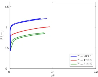
Fig. 6 shows the results of tensile and compressive tests at various temperatures. While the yield stress decreases quasi-linearly as the temperature rises (see Fig. 7), the hardening rate does not seem to be affected by the temperature under isothermal conditions.
As mentioned in the introduction, the yield stress dependence on the temperature can have a strong impact on the self-heating consequences at high loading rates. Indeed, the competition between thermal softening and plastic strain as well as strain rate hardening at high loading rates will determine the potential instability of the material.
* Effect of stress triaxiality ratio χ Fig. 8 shows the force vs. nominal strain for the specimens in Fig. 2. The resistance and the
ductility are highly dependent on the notch radii and resulting stress state, as expected. The highest force and lowest nominal strain at
fracture is observed for the double notched specimen (χ ’1.0), while both single notch specimens exhibit the same peak load (χ ’ 0.5–0.6), but a lower fracture strain for the smaller notch radius. As for the shear specimen, a comparatively lower load and higher nominal strain at fracture is observed with respect to the other geometries.
The experimental scatter is probably due to small deviations from the nominal specimens dimension and to the macrozones present in the material (see Fig. 1b).
2.3.2. Reversed loading: σKH vs σIH
In order to quantify the respective contributions of isotropic and kinematic hardening, tension-then-compression and compression- then-tension tests are carried out. These two different sequences also allow to check that the strength differential deduced from separate tension and compression tests on different sample geometries is retrieved when a unique sample geometry and test setup is used.
As an example, Fig. 9 shows the recorded stress-strain loops during 2.5 tension-compression cycles along the rolling direction. The isotropic and kinematic components of the material hardening can be deduced from the stress for which the stress-strain curve during unloading departs from linearity by more than a given offset (Dickson et al., 1984). For example, for an offset of δϵp ¼10 4, the
kinematic hardening values were found to contribute for more than 30% to the flow stress in Ti–6Al–4V. Yet, changing the offset results in a change of the relative contributions.
Fig. 5. Stress vs plastic strain. Tension and compression. Influence of the strain rate. T ¼ 25 �C, Rolling direction RD. The dots in the high strain rate
Fig. 6. Stress vs plastic strain. Influence of temperature. j_ϵj ’ 103s 1, Rolling direction RD. Similar effects were observed for the other directions
tested as well as compression loading.
2.3.3. Multi-step relaxation loading: σv
As deduced from tests carried out at different strain rates, a strain rate-induced overstress is present, see Fig. 5 at room temperature. A series of stress relaxation periods are therefore introduced during tensile as well as compressive tests, in order to extract the viscous component of the flow stress. The displacement-controlled tests are interrupted at selected strain amounts and the total deformation of the specimen remains constant. A drop in stress is recorded due to viscous relaxation and the test is resumed when the stress level has reached a steady state.
In Fig. 10 are plotted the stress-strain curves obtained from the multi-step relaxation loading. The dotted lines are obtained by interpolation between the end-points of the relaxation periods and represent the rate independent part of the flow stress. By sub-tracting it from the total stress, the viscous component can be determined from Equation (1) via
Fig. 8. Load vs strain. Tension. Influence of stress triaxiality. _ϵ ’ 10 3s 1, T ¼ 25 �C, Transverse direction TD.
σv¼σ ðσKHþσIHÞ (2)
According to Fig. 10, the viscous stress remains constant along the deformation in tension and compression. Furthermore, no anisotropy is found in terms of the relaxed stress. Therefore, the viscous component is considered independent of the loading direction and of the deformation. This enforces the previous simplification in Equation (1) of additive decomposition of the stress in a strain hardening and a viscous component.
Slight differences in viscous behavior in tension and in compression can be however noticed. To check if these differences are significant or an artifact due to the differences in testing devices and specimens geometries, the cylindrical specimens used for the reversed loading are employed to measure the relaxed stress both in tension and in compression. Fig. 11 shows the results of a compression-tension test with two relaxation periods in tension and compression. The viscous stress, plotted in red, does not show a significant dependence on the loading direction.
Some works have reported a temperature dependence of the strain rate sensitivity, see e.g. (Tuninetti and Habraken, 2014)). For the material under consideration in the present study, this effect is weak enough to be neglected.
2.4. Analysis and discussion
By extrapolating the steady-state curves (dotted lines) in Fig. 10, the rate independent initial yield stress at room temperature can be estimated for each loading direction. It can then be subtracted from the flow stress at various strain rates so as to determine the
Fig. 10. Stress vs plastic strain. Tension and compression. Multi-step relaxation tests. The drop in stress as the static state is achieved is defined as
viscous stress. Similarly, the viscous stress measured in the relaxation tests can be used to obtain from Equation (1) the rate inde-pendent stress σKH þσIH ¼σ σv.
In this section, the effects of anisotropy, strain hardening and temperature on the rate independent stress are analyzed as well as the viscous stress.
2.4.1. Plastic anisotropy and strength differential
Fig. 12 shows the yield surface in the (σRD, σTD) plane at various plastic strain amounts. In the case of the diagonal direction, the Cauchy stress components with respect to the rolling and transverse axes are plotted. As for the normal direction ND, the equivalent biaxial state is used. For the sake of comparison, the von Mises yield surface passing through the yield stress along the rolling direction RD is plotted to quantify the degree of anisotropy. Von Mises criterion clearly underestimates the yield stresses in compression (the compression under the normal direction ND is shown in the top right quadrant as a biaxial tensile state). As for the orthotropy, dif-ferences are more subtle. The yield stress in the transverse direction TD tends to be underestimated whereas those in the normal ND and diagonal DD directions are overestimated by the isotropic yield criterion. As the deformation increases, the misfit with von Mises criterion grows larger as seen in Fig. 12.
Fig. 11. Stress vs strain. Compression-tension test with four relaxation periods on a cylindrical specimen. j_ϵj ’ 5 � 104s 1, T ¼ 25 �C, Rolling
direction RD. The viscous stress is plotted in red. (For interpretation of the references to colour in this figure legend, the reader is referred to the Web version of this article.)
Fig. 12. Yield locus in the (σRD, σTD) plane, after viscous component removal. j_ϵj ’ 10 3s 1, T ¼ 25 �C. The loading in the normal direction is
2.4.2. Strain hardening
The first cycle from Fig. 9 is reconsidered here after removing the viscous component, to highlight the contributions of the isotropic and the kinematic hardening. The compressive part of the cycle has been inverted and is compared with the tension and compression monotonic stress-strain curves. As observed in Fig. 13, a nonlinear kinematic hardening produces a progressive yielding during the load reversal. As the cyclic curve goes into compression, a permanent offset with respect to the monotonic compression appears, as a result of the Bauschinger effect.
2.4.3. Strain rate hardening
The viscous component from the curves in Fig. 5 is plotted versus the strain rate in a logarithmic scale on Fig. 14 for the tension and compression tests. The result evidences the linear evolution of the viscous component with strain rate (in the log scale). The Norton- Perzyna law is accordingly suitable to reproduce the observed results. It is expressed as
σv¼Yvκ_1=nv (3)
2.4.4. Thermal softening
As shown in Fig. 6, the flow stress monotonically decreases with increasing temperature. Although the evolution of the flow stress with respect to temperature seems linear (see Fig. 7), within the limited range of temperatures investigated, a linear extrapolation would predict negative stress values before the melting point. A power law is commonly used in literature, and it ensures a positive stress until melting (Long�ere, 2018):
σ∝1 〈T Tref Tm Tref
〉mT (4)
where mT is a material parameter, Tm ’1630 �C the melting point and T
ref ¼25 �C the reference temperature. The Macaulay brackets
〈x〉 ¼ maxð0; xÞ are used.
Under low strain rate loading the conditions are isothermal, whereas under high strain rate loading, they are (quasi) adiabatic. As a consequence, the heat generated by plastic dissipation is not evacuated fast enough by conduction, leading to a local temperature rise and the material is subject to thermal softening along the deformation process. Self-heating is usually estimated by considering that a fraction of the plastic work rate is converted into heat:
ΔT ’ β
ρc Z
κ
σdκ (5)
where ρ is the mass density and c is the specific heat of the material. β represents the inelastic heat fraction also called Taylor-Quinney
coefficient (Taylor and Quinney, 1934). The latter is often assumed constant with values typically ranging between 0.8 and 1. Experimental estimates of β for Ti–6Al–4V may be completely different from an author to another, see e.g. Mason et al. (1994) and (Macdougall and Harding, 1999), while showing that β does not keep a constant value along the deformation process. In absence of further information on the right value of β for the material under consideration, we are here assuming that β ¼ 0.9.
Equivalent isothermal stress-strain curves may be obtained from adiabatic stress-strain curves by removing the self-heating induced thermal softening. By assuming β ¼ 0.9 and using Fig. 7, isothermal dynamic compression curves can be estimated, see Fig. 15.
Fig. 13. Stress vs strain. Strain hardening comparison between the monotonic tests and the load reversal test. j_ϵj ’ 103s 1, T ¼ 25 �C Rolling
Accordingly, isothermal, quasi-static and dynamic curves exhibit a similar strain hardening.
3. Constitutive modeling
The extensive experimental campaign detailed in the previous section has evidenced that the Ti–6Al–4V grade under consideration is subject to significant (i) anisotropic plasticity which manifests through loading direction dependence, kinematic hardening and strength differential, (ii) isotropic strain hardening, (iii) rate dependence and (iv) thermal softening. Starting from the experimental observations, a constitutive model accounting for the above mentioned effects is built within the irreversible thermodynamics framework. More generally, the aim of the present work is to develop a constitutive model able to describe the behavior of metals and alloys within a wide range of strain, strain rate, temperature and loading path.
Kinematic considerations are first specified in the context of large elastic-plastic deformation. The general irreversible thermo-dynamics framework is then applied for phenomenologically describing the consequences of the underlying conservative and dissi-pative mechanisms. Eventually, constitutive equations are applied to the Ti–6Al–4V grade under consideration.
Fig. 14. Stress at 2% of plastic strain vs plastic strain rate. Tension and compression. At this plastic strain amount self-heating induced softening
3.1. Finite strain framework
Moderately large elastic-plastic strains have been observed during the experimental campaign, implying a nonlinear geometric formulation. The deformation gradient F describes the transformation from the initial (undeformed) configuration to the current (deformed) configuration of the particle coordinates of any point belonging to the material body. As suggested by (Lee and Liu, 1967; Lee, 1969), the deformation gradient F may be multiplicativally decomposed into an elastic contribution Fe and a plastic contribution Fp:
F ¼∂x
∂X ¼F
eFp (6)
where X and x ðX ; tÞ represents the particle coordinates in the initial and current configurations, respectively. In this context, Fe represents the transformation between the virtually elastically unstressed (intermediate) configuration and current configuration, and Fp the transformation between the initial configuration and virtually elastically unstressed (intermediate) configuration.
We are here considering an intermediate configuration virtually unstressed by a pure elastic stretching Ve 1, yielding
F ¼ VeQ Fp (7)
where Q represents an orthogonal transformation (rotation). The velocity gradient l accordingly reads (see Long�ere et al. (2003)) l ¼∂v ðx Þ
∂x ¼ _F F
1¼V▿e Ve 1þW þ VeF_pFp 1Ve 1 (8)
where v is the particle velocity and where W ¼ _Q QT represents the rate of the orthogonal transformation. The decomposition of the deformation gradient l into a symmetric part d and a skew-symmetric part w , viz. l ¼ d þ w , yields
� d ¼ ½l�S¼deþdp w ¼ ½l�SS¼W þ weþwp (9) where ( de¼�V▿e Ve 1�S we¼�V▿e Ve 1�SS; ( dp¼�VeF_pFp 1Ve 1�S wp¼�VeF_pFp 1Ve 1�SS (10)
yielding the following expression for the rotation rate W
W ¼ _Q QT¼w ðweþwpÞ (11)
Moreover, the objective derivative a▿
of any second order tensor a reads a
▿
¼ _a W a þ a W (12)
Under small elastic strain assumption, Equation (10) reduces to � de¼▿Ve we¼0 ; ( dp¼�F_pFp 1�S wp¼�F_pFp 1�SS (13)
In addition, assuming tentatively negligible effect of the spin wp in regards with the spin w (see the assumption of moderate plastic
strain in Schieck and Stumpf (1995)), Equation (11) reduces to
W ¼ w (14)
where the assumption of negligible effects of anisotropy is also used (Mandel, 1973).
According to the decomposition of the deformation gradient F in Equation (7), when working with respect to the current configuration, it is needed to use the Zaremba-Jaumann objective derivative. Alternatively, it is possible to work with respect to the Q -rotated or co-rotational configuration, by means of a push forward and a pull back rotations (Hughes and Winget, 1980; Long�ere, 2019). The latter method is used in the following. The rate equations of the constitutive model are consequently formulated by using time derivatives with respect to the co-rotational frame:
_ a
Q¼Q Ta▿
Q (15)
For example the Cauchy stress would read in the context of temperature independent hypo-elasticity as
σ ▿ ¼C : de → σ_ Q¼C : _ϵ e Q (16)
In the sequel, the subscript ⋅Q is dropped for simplicity. 3.2. Irreversible thermodynamics framework
Constitutive state laws and complementary laws respectively derived from the state and dissipation potentials are expressed in this subsection.
3.2.1. State potential and constitutive state laws
The internal variable procedure is herein applied within the irreversible thermodynamics framework to model the thermo- mechanical behavior of the Ti–6Al–4V grade under consideration. The instantaneous state of the material is assumed to be well described via the Helmholtz free energy Ψ whose arguments are the absolute temperature T, the elastic strain tensor ϵe, the isotropic hardening variable (also called cumulated plastic strain) κ, and the kinematic hardening variable α. Therefore, the Helmholtz state
potential can be decomposed into four parts: a recoverable energy Ψe, a purely thermal part ΨT and two stored energies corresponding to the isotropic and kinematic hardening contributions, ΨpI and ΨpK, see (Halphen and Nguyen, 1975). Considering tentatively state uncoupling between the two mechanisms of plasticity and between them and elasticity, the Helmholtz free energy Ψ is taken of the form
Ψðϵe;κ;α;TÞ ¼ Ψ
eðϵe;TÞ þ ΨTðTÞ þ ΨpIðκ; TÞ þ ΨpKðαÞ (17)
where ΨpK is taken as temperature independent. The specific contributions to the state potential are defined as 8 > > > > > > > > > > < > > > > > > > > > > : ρΨeðϵe;TÞ ¼ 1 2ϵ e:C : ϵe αKðT T 0ÞtraceðϵeÞ ρΨT¼ ρc 2T0 ΔT2 ρΨpIðκ; TÞ ¼ hðκÞgðTÞ ρΨpKðαÞ ¼ 1 3Cα:α (18)
where ρ is the mass density, C is the elasticity stiffness fourth order tensor, with Cijkl ¼λδijδklþμ δikδjlþδilδjk �
, λ and μ being the Lam�e
coefficients, K the bulk modulus, with K ¼ λ þ2
3μ, α the thermal dilatation coefficient, T0 the initial temperature, and c is the specific
heat. hðκÞ and gðTÞ are the stored energy of cold work and the thermal softening function, respectively, and the scalar C is a kinematic hardening-related parameter.
The thermodynamic forces derived from the state potential with respect to their conjugate variables are given by the constitutive state laws defined below.
8 > > > > > > > > > > > > > > > > > > > > > > < > > > > > > > > > > > > > > > > > > > > > > : σ¼ρ∂Ψ ∂ϵe � � � � κ;α;T ¼ρ∂Ψe ∂ϵe � � � � T ¼C : ϵe αKðT T 0ÞI ρs ¼ ρ∂Ψ ∂T � � � � ϵe;κ;α ¼ ρ ∂Ψe ∂T � � � � ϵe þ∂ΨT ∂Tþ ∂ΨpI ∂T � � � � κ ! ¼αKtraceðϵeÞþρc T0 ΔT hðκÞg0ðTÞ r ¼ρ∂Ψ ∂κ � � � � ϵe;α;T ¼ρ∂ΨpI ∂κ � � � � T ¼h0ðκÞgðTÞ X ¼ρ∂Ψ ∂α � � � � ϵe;κ;T ¼ρ∂ΨpK ∂α � � � � T ¼2 3Cα (19)
where σ is the Cauchy stress tensor, s the entropy, r the isotropic hardening force and X the kinematic hardening force.
Finally, the Gibbs relation reads
ρΨ ¼_ σ : _ϵeþr _κ þ X : _α ρs _T (20)
3.2.2. Dissipation and complementary laws
Injecting the Gibbs relation into Clausius-Duhem inequality and using _ϵ ¼ _ϵeþ _ϵp yield the following expression for the intrinsic dissipation
D ¼σ : _ϵ ρð _Ψ þ s _TÞ
¼σ: _ϵp r _κ X : _α �0 (21)
which involves force-related quantities A ¼ ðσ;r; X Þ and flux-related quantities _a ¼ ð_ϵp; κ;_ α_Þ. In the context of the normality rule, the dissipation may be rewritten in the following form
D ¼A _a ¼ A_λ∂F
∂A�0 (22)
where F is the plastic potential meeting the required conditions of positiveness and convexity and where _λ is the positive plastic multiplier. In the context of rate dependent non-associated plasticity, _λ is assumed to derive from a dissipation potential ΩðfÞ, viz. _λ ¼
∂Ω=∂f, where f represents the yield function.
The yield function f and plastic potential F are written of the form f ðσ;r; X ; …Þ ¼σeqðσ;X ; …Þ σyðr; …Þ ¼σvð _κ; …Þ � 0
Fðσ;r; X ; …Þ ¼ f þ bfðX Þ (23)
where σeq is the transformed equivalent stress accounting for the different sources of plastic anisotropy, σy the rate independent yield stress, σv the strain rate induced overstress or viscous stress, and where … represents other arguments defined later. bfðX Þ is a function involving non-linearity in kinematic hardening.
The normality rule accordingly yields 8 > > > > > > > > < > > > > > > > > : _ ϵp¼ _λ∂F ∂σ¼ _λ ∂σeq ∂σ ¼ _λn with n ¼ ∂σeq ∂σ _ κ ¼ _λ∂F ∂r¼ _λ ∂f ∂r¼ _λ _ α¼ _λ∂F ∂X ¼ _λ � ∂f ∂X þ ∂bf ∂X � ¼ _λm with m ¼ � ∂σeq ∂X þ ∂bf ∂X � (24)
These laws are completed by the temperature rise coming from adiabatic self-heating under high strain rate loading assuming negligible contributions of thermo-elastic and thermo-plastic couplings (Long�ere and Dragon, 2009). Temperature rise is estimated from dissipation in Equation (21), see Long�ere and Dragon (2008), according to
3.3. Constitutive equations
Quantities introduced in the previous subsection are now specified for the material under consideration in agreement with the experimental observations.
3.3.1. Transformed equivalent stress σeq
Plastic anisotropy entails a loss of coaxiality between the plastic strain rate and the stress deviator. As the plastic strain rate is derived from the transformed equivalent stress according to the normality rule, the plastic anisotropy effects are accounted for in the expression of the transformed equivalent stress. It is reminded that in the present case plastic anisotropy manifests through (i) loading direction dependence, (ii) kinematic hardening, and (iii) strength differential.
We are here considering the transformed equivalent stress σeq as a function of three variables, namely the current Cauchy stress second order tensor σ, the back stress second order tensor X , and a fourth order tensor accounting for the texture-induced orthotropy
A.
σeq¼σeqðσ;X ; AÞ (26)
Each source of anisotropy is first studied independently of the others and then a combination of the three sources is proposed. * Texture-induced initial orthotropy: X ¼ 0
Following Karafillis and Boyce (1993), we introduce the transformed stress Σ ¼ A :σ also denoted as the Isotropy Plasticity
Equivalent (IPE) stress. The fourth order tensor A is a linear multiplicative operator involving potential plastic orthotropy. In the case of an isotropic material, the operator reduces to the identity tensor, viz. A ¼ I. As a consequence, the transformed stress reads
σeqðσ;X ; AÞ ¼σeqðΣ ; X Þ (27)
Table 1 reports two definitions of the transformed equivalent stress aiming at accounting for anisotropic plasticity: (i) by incor-porating the tensor A directly in the expression of the equivalent stress, as proposed by Hill (1948), and (ii) by incorporating it at the stress level, as proposed by Karafillis and Boyce (1993).
The fourth order tensor accounting for anisotropic plasticity can be simplified as a 6 � 6 matrix according to major and minor symmetries while stress second order tensors are reduced to vectors according to Voigt or Bechterew notations.
A ¼ 2 6 6 6 6 6 6 4 A11 A12 A13 A12 A22 A23 A13 A23 A33 A44 A55 A66 3 7 7 7 7 7 7 5 (28)
In case of pressure independent-orthotropic plasticity, following condition in Equation (29) for anisotropy coefficients in Equation (28) is required and Hill48 (Hill, 1948) orthotropic matrix is retrieved with 6 independent anisotropy coefficients.
8 < : A11¼ ðA12þA13Þ A22¼ ðA12þA23Þ A33¼ ðA13þA23Þ (29) We are here adopting the 9-anisotropy-coefficient approach in Equation (28) and the pressure independence will be described by applying the linear transformation A to the stress deviator tensor and not to the stress tensor itself, see Equation (32) and Table 2 later on.
* Kinematic hardening-induced evolving anisotropy A ¼ I
The approach commonly adopted when dealing with kinematic plastic hardening is to consider the translation of the yield surface
Table 1
Definitions of transformed equivalent stress in the case of ortho-tropic plasticity.
Hill (1948) K&B (1993)
σ2eq¼1
2σ:A :σ Σ ¼A :σ σ2eq¼1
by means of the deviatoric back stress X . For instance, the transformed equivalent stress would read σ2 eq¼ 3 2ðs X Þ : ðs X Þ ¼ 3 2^s : ^s (30) where. ^s ¼ ðs X Þ
* Strength differential-induced initial anisotropy A ¼ I & X ¼ 0
The strength differential between tension and compression can be assumed to be a type of anisotropy. As mentioned in the introduction, CPB06 (Cazacu et al., 2006), Khan (Khan et al., 2012) and Long�ere (Long�ere et al., 2012) propose different methods for describing this effect. In this study, the CPB06 model (Cazacu et al., 2006) is chosen as it allows for a simple definition of the yield surface without resorting to the Lode angle or a coupling with the viscous component. The CPB06 isotropic yield surface adds a strength differential parameter k to the definition in Karafillis and Boyce (1993) resulting in the form
σeqa¼
1 m0a
fðjS1j kS1Þaþ ðjS2j kS2Þaþ ðjS3j kS3Þag (31)
where Sp are the eigenvalues of the stress tensor σ, k is the main parameter defining the material asymmetry, a is a shape parameter of
the yield surface, see Hosford (1972) and m0 is a model constant.
The Karafillis and Boyce (1993) generalized yield criterion can be recovered for k ¼ 0 (and the Mises criterion with a ¼ 2). The CPB06 criterion in Equation (31) can thus be considered as an extended distortion (without a rotation) of such surface.
* Complete transformed equivalent stress A 6¼ I & X 6¼ 0
In order to couple kinematic hardening and plastic orthotropy, two approaches can be considered, see Table 2. Following Baltov and Sawczuk (1965), the back stress is first subtracted from the deviatoric stress tensor and the Hill criterion is then applied. Alter-natively, Karafillis and Boyce (1993) make use of their linear operator to transform the difference between the stress tensor and the back force.
On the other hand, coupling plastic orthotropy and strength differential may be achieved following CPB06 (Cazacu et al., 2006) approach. Indeed, the authors apply a linear transformation to the stress deviator: Σp is defined as the eigenvalues of the transformed tensor Σ ¼ A : s which replaces s in Equation (31), see Table 2. The authors initially proposed a symmetric definition of the 6 � 6 matrix representation of the tensor A as in Equation (28), although further simplifications using a Hill-like matrix can be made to model the orthotropy as found in (Stewart and Cazacu, 2011).
We are here coupling kinematic hardening, plastic orthotropy and strength differential by combining Karafillis and Boyce (1993) and CPB06 (Cazacu et al., 2006) methods. For that purpose, we are defining the transformed stress eigenvalues as follows, see Table 2.
b
Σp¼eigð bΣ Þ;
b
Σ ¼ A : ðs X Þ (32)
Therefore, the complete anisotropic criterion reads
σeqa¼
1 m0a
fðjbΣ1j k bΣ1Þaþ ðjbΣ2j kbΣ2Þaþ ðjbΣ3j k bΣ3Þag (33)
The constant m0 is defined such that the equivalent stress is equal to the uniaxial stress in tension (compression) if k > 0 (k < 0) for
an isotropic material, i.e. A ¼ I. m0a¼ � 2 3ð1 jkjÞ �a þ2 � 1 3ð1 þ jkjÞ �a (34) The coefficients A55 and A66 are herein assumed to be 1 due to the lack of information for shear along the normal direction (an
alternative approach is to consider A44 ¼A55 ¼A66 as done by Tuninetti and Habraken (2014)). 3.3.2. Viscous stress σv
Regarding the rate dependent formulation, the experimental results show the existence of a strain rate induced overstress
inde-Table 2
Examples of anisotropic plasticity-oriented transformed equivalent stress.
B&S (1965) K&B (1993) CPB06 Present approach
^ s ¼ s Xσ2eq¼1 2^s : A : ^s bΣ ¼A ðσ X Þσ2eq¼1 2bΣ : bΣ Σp¼eigðΣ ÞΣ ¼ A : sσeq¼σeq Σp;k � b Σp¼eigð bΣ Þ b Σ ¼A : ðs X Þσeq¼σeq bΣp;k �
pendent of the anisotropy axes and plastic strain and whose temperature dependence within the temperature range of interest is negligible. The Norton-Perzyna law is proposed to describe such behavior (Norton, 1929).
σv¼Yvκ_1=nv (35)
where Yv and nv are material coefficients.
By following the approach in Perzyna (1966), the potential described in Equation (22) is accordingly of the form Ωðf Þ ¼ 1
nvþ1
〈f Yv
〉nvþ1 (36)
Indeed, by combining 24.2 and 36, the Norton-Perzyna law in Equation (35) is retrieved _ κ ¼ _λ ¼∂Ω ∂f ¼〈 f Yv 〉n¼〈σv Yv 〉n (37)
3.3.3. Rate independent yield stress σy
The radius of the elasticity domain is defined as a temperature dependent initial threshold stress σy0ðTÞ plus the stress related to the isotropic hardening rðκ; TÞ. Both the initial threshold stress and isotropic hardening force are assumed to depend on temperature according to the same thermal softening function gðTÞ:
σy¼σy0ðTÞ þ rðκ; TÞ ¼ gðTÞRðκÞ (38)
3.3.3.1. Strain hardening. For the definition of the isotropic hardening, the Swift (power) law and the Voce (exponential with satu-ration) law are widely used (see (Roth and Mohr, 2018; Roth and Mohr, 2016) for a linear combination of both). For the material under consideration, some initial constant calibration (not shown here) from the monotonic tests have shown that Swift law fits well the experimental curves. On the other hand, Chun et al. (2002) and Carbonni�ere (Carbonni�ere et al., 2009) have shown that a coupling between isotropic and kinematic hardening is well described by adding a negative Voce-type exponential law in the expression of the strain hardening function.
Therefore, a combination of Swift and (negative) Voce expressions is herein considered in view of coupling isotropic and kinematic hardening. The adopted forms for the strain hardening function h0
ðκÞin Equation (19) and radius RðκÞ in Equation (38) read h0ðκÞ ¼ Q0ðϵ0þκÞn C Dð1 expð DκÞ Þ RðκÞ ¼ R0þh 0 ðκÞ (39) where R0, Q0, ϵ0 and n are the Swift law-related postive constants and C and D are (negative) Voce law-related positive constants.
3.3.3.2. Thermal softening. As previously evidenced by the experimental campaign, the thermal softening function gðTÞ is of the form gðTÞ ¼ 1 〈T Tref
Tm Tref
〉mT (40)
where Tm is the melting point and Tref and mT material constants. 3.3.4. Complementary laws
Following the decomposition made in Equation (24), the plastic strain rate is expressed as _
ϵp¼ _κ∂σeq
∂σ ¼ _κn (41)
where n ¼∂σeq=∂σ represents the yield direction. It can be shown that the explicit expression for n is
n ¼X 3 p¼1 " 1 ma 0 ���bΣp � � k bΣ p σeq �a 1 sgn bΣp � k� # J : A : vp�vp � (42) where vp is the eigenvector corresponding to the eigenvalue bΣp. The outer product ⋅�⋅ is here used and J is the fourth order tensor projecting σ onto its deviatoric plane s . The deviator operator J is defined in the index form as
Jijkl¼ � 1 2 δikδjlþδilδjk � 1 3δijδkl � (43) To describe nonlinear kinematic hardening, function bfðX Þ in Eq (23) is taken of the form (see (Lemaitre and Chaboche, 1994))
bf ðX Þ ¼3D
4CX : X (44)
The rate of the kinematic hardening variable in Equation (24) accordingly reads _ α¼ κ_ � ∂f ∂Xþ 3D 2CX � ¼ _κm (45)
It can be easily shown that ∂σeq=∂X ¼ n . With this expression, the normal tensor m recovers the non linear definition seen in
Armstrong and Frederick (1966) and Chaboche (1986):
m ¼ n 3D
2CX _
α¼ _ϵp D_κα (46)
It is noteworthy that the material constants C and D coincide with the Voce law constants in Equation (39).
Injecting the different expressions in Equations (41) and (46) into Equation (25) yields the following expression for the temperature rise _T ¼1 ρc � σeq r þ 2 3CDα:α � _ κ (47)
As mentioned previously, the temperature rise is usually estimated via the inelastic heat fraction β, also known as the Taylor- Quinney coefficient (Taylor and Quinney, 1934), defined as the fraction of the plastic work rate converted into heat, or
_T ¼β
ρcσvmκ_ (48)
The coefficient β is often arbitrarily assumed constant with a value typically ranging from 0.8 to 1.0 without much physical motivation to back it up (Vadillo et al., 2008) and despite many experimental evidences of its dependence on strain and even strain rate and temperature itself (see Macdougall and Harding (1999)). As done in Long�ere (2018), this coefficient may be deduced consistently from the constitutive model. In the present case, it reads
β ¼σeq r þ
2 3CDα:α
σvm (49)
This expression for β intrinsically accounts for potential dependence on strain, strain rate and temperature and is used in the sequel. In the present work, following a thermodynamic approach, the inelastic heat fraction β is consistently deduced from the constitutive model and accordingly evolves along the loading path. For high strain rate tension loading, starting from a value close to 0.95, β is slightly decreasing with increasing strain, reaching a value close to 0.8 at 0.3 of plastic strain. This evolution for β is close to the one reported in Rosakis et al. (2000).
3.4. Summary of the constitutive equations
Rate equations of the constitutive model are summarized below. 3.4.1. Constitutive state laws
8 > > > < > > > : _ σ ¼C : _ϵe αK _T _ X ¼2 3C _α _ r ¼ h00 ðκÞgðTÞ_κ þ hðκÞg0ðTÞ _T (50) where 8 > > > < > > > : hðκÞ ¼ Q0 n þ 1ðϵ0þκÞ nþ1 C DðDκ expð DκÞ Þ gðTÞ ¼ 1 〈T Tref Tm Tref 〉mT (51) 3.4.2. Yield function f ð bΣ ; k; rÞ ¼σeq Σbp;k � ½R0gðTÞ þ rðκ; TÞ � ¼σvð _κÞ � 0 (52)
where σeq bΣp;k � ¼ 1 m0a fðjbΣ1j k bΣ1Þaþ ðjbΣ2j k bΣ2Þaþ ðjbΣ3j k bΣ3Þag b Σp¼eigð bΣ Þ b Σ ¼ A : ðs X Þ (53) 3.4.3. Complementary laws 8 > > > > > > > > < > > > > > > > > : _ κ ¼ 〈f Yv 〉nv _ εp¼ _ κn _ α¼ _εp D_κα _ T ¼βσvm ρc κ_ (54) where 8 > > > > > > > > > > > < > > > > > > > > > > > : n ¼X 3 p¼1 " 1 ma 0 ���bΣp � � k bΣp σeq �a 1 sgn bΣp � k� # J : A : vp�vp � β ¼σeq r þ2 3CDα:α σvm σvm¼ ffiffiffiffiffiffiffiffiffiffiffiffiffi 3 2s : s r (55) 3.4.4. Initial conditions 8 > > < > > : ϵpð0Þ ¼ 0 X ð0Þ ¼ 0 rð0Þ ¼ 0 Tð0Þ ¼ T0 (56) 3.4.5. Material constants Elasticity: E ¼ 110 GPa, ν ¼0.3 Anisotropy (9): a, k, A11, A22, A33, A44, A12, A23, A13, A55 ¼A66 ¼1 Viscosity (2): Yv, nv Hardening (6): R0, Q0, ϵ0, n, C, D Temperature (2): mT, Tref ¼25 �C, T m ¼1600 �C
4. Model implementation, identification and validation
This section aims at showing the numerical procedure used to implement the material constitutive equations as a user material subroutine in a commercial finite element code (LS-DYNA) using an explicit time integration of the rate equations. The identification of the material coefficients using the commercial software Z-set is then pursued so as to check the validity of the model as well as its limitations. Finally, a validation using notched specimens is performed.
4.1. Numerical procedure
The numerical time integration of the constitutive equations starts with a finite differences scheme in the co-rotational frame. This means a push forward operation has been previously performed. The elastic strain rate is therefore approximated as an increment between times ti and tiþ1 which can be decomposed in a volumetric part (not playing a role in the viscoplastic problem here defined) and a deviatoric part.
( _ p ¼ K _ϵvþ3αK _T ¼ K _ϵT ϵ_v � _ s ¼ 2μϵ_e dev → ( Δp ¼ K ΔϵT Δϵ v � Δs ¼ 2μΔϵe dev (57)
where _ϵT¼3αT ¼ 3_ αð _Tisoþ _TadiaÞis the thermal strain rate related to the increase in temperature (i) under isothermal conditions, i.e. a global external temperature and (ii) due to the adiabatic self-heating of the material. Hence, two thermal strain increments can be defined: ΔϵT
iso¼3αΔTiso and ΔϵTadia ¼3αΔTadia.
The total strain increment is accordingly decomposed in an elastic, plastic and two thermal components. Δϵ ¼ ΔϵeþΔϵpþ1 3Δϵ T isoI þ 1 3Δϵ T adiaI (58)
The corresponding volumetric and deviatoric parts are (
Δϵv¼traceðΔϵ Þ ¼ traceðΔϵeÞ þΔϵTisoþΔϵTadia
Δϵ dev¼Δϵ e devþΔϵ p dev (59) The strategy used to integrate the equations is based on a two-step elastic prediction-plastic correction algorithm (Simo and Hughes, 1998) (see Fig. 17). An explicit integration of the total strain increment from the equilibrium equations is considered as the input variable in the algorithm.
The plastic correction is carried out with a direct integration of the Perzyna formulation (see (Perzyna, 1966)). The yield surface value to be used is a first order approximation based on its value at the previous increment and an estimation of its increment.
_ κ ¼ 〈f Yv 〉nv→ Δκ ¼ 〈f iþ1=2 Yv 〉nvΔt ¼ 〈f iþ1 2Δf Yv 〉nvΔt (60)
In order to integrate Equation (60), an approximation of the yield surface increment is done by expanding its partial derivatives with respect to its arguments.
Δf ¼∂f ∂σ:Δσþ ∂f ∂X :ΔX þ ∂f ∂κΔκ þ ∂f ∂TΔT ¼n : Δstrial 2μn : n þ g0 Ti�R κi�∂T ∂κ � � � � i þg Ti�R0 κi�þn :∂X ∂κ ! Δκ0 (61)
An initial estimation of the plastic strain increment is defined as Δκ0¼〈
fi
Yv
〉nvΔt (62)
The partial derivative of the temperature with respect to the plastic strain is obtained by using the reduced heat expression in Equation (25). ∂T ∂κ � � � � i ¼β iσi vm ρc (63)
The reason for this first order approximation is to delay instabilities as the imposed strain increments become large. Fig. 16 shows a comparison between the forward Euler integration (using the yield function at the time instant tn) and the first order approximation just described. When compared to an implicit solution, where convergence to the exact solution is presumed, the forward Euler shows instabilities for very high strain rates. Some slight oscillations can be observed on the stress-strain curve as well as some larger ones when computing the plastic strain rate. Therefore, a first-order approximation of the yield surface at the time instant tnþ1/2 provides with a much closer and more stable solution with respect to the implicit one without recurring to a computationally costly implicit loop.
Once the cumulative equivalent plastic strain κ is integrated, the rest of the state variables, i.e., the kinematic variable and the temperature can be updated. A discrete approximation of Equations (45) and (48) as well as Equation (46) is considered:
8 > > > < > > > : Δα� ¼ � ntrial 3D 2CX i � ΔκΔT ¼1 ρcβ iσi eqΔκ (64)
Finally the update of the stress state is performed by means of a correction where the plastic strain and thermal increment contributions are subtracted. This return algorithm uses the yield direction at the trial stress state under the assumption that a radial correction is sufficient to correct the stress.
Fig. 16. Uniaxial tensile simulation at the element scale.
( Δp ¼ ΔptrialþKΔϵT vI ¼ Δp trialþKαΔTI Δs ¼ Δstrial 2μΔϵp dev¼Δs trial 2μntrialΔκ (65)
A summary of the numerical integration is described in the flowchart depicted in Fig. 17. 4.2. Model constants calibration at the volume element scale
The commercial software Z-set is chosen to carry out the identification of the material coefficients. Three stages are considered for the calibration of the material parameters: (i) 9 coefficients for the anisotropy (using the von Mises criterion as the starting point of the optimization, i.e. a ¼ 2, k ¼ 0 and Aij ¼Iij), (ii) 2 coefficients for the viscosity (once the anisotropy has been identified) and finally (iii) 7 coefficients for the strain hardening and thermal softening identification.
A volume element under uniaxial tension and compression at various strain rates along various directions is considered for the calibration. The inverse-problem identification of the material constants is performed using a gradient-based optimization method (Andrade-Campos et al., 2007). In particular, the Levenberg-Marquardt algorithm (Marquardt, 1963) is employed for the least-square minimization between the numerical and experimental results:
Cðp Þ ¼1 2 XT i¼1 XN j¼1 wj � σEXP j ðtiÞ σNUMj ðp ; tiÞ �2 (66) where C is the cost function to minimize, p the set of material constants to identify, wj a weight parameter and the subscripts i and j are used to denote different times and tests respectively. For confidentiality reason, the values of the coefficients are not given. 4.2.1. Calibration of the orthotropy and strength differential related coefficients
In order to identify the anisotropy, the parameters a, k, A11, A22, A33, A44, A12, A23 and A13 are fitted. For that purpose, the stress-
strain tension and compression curves from the monotonic quasi-static tests run at 10 3 s 1 are used. Fig. 18 shows the result of such
identification. The tension-compression differential is well captured as well as the orthotropy for both types of loadings. 4.2.2. Calibration of the viscoplasticity related coefficients
Only the viscosity coefficients Yv and nv are considered in this stage. As seen with the dynamic tensile testing in Fig. 5, the combined effect of self-heating induced softening and the poor camera resolution is responsible for a poor measurement of the hardening curves. For this reason, the viscosity identification uses only compression stress-strain curves from monotonic quasi-static and dynamic loading plus the tension curves in the quasi-statique regime. Fig. 19 shows a comparison with the identified numerical viscous model with the experimental data. The Norton law proves itself the right approximation to reproduce the overstress observed in the experiments.
Fig. 19. Stress at 2% of plastic strain vs plastic strain rate. Tension and compression. Viscoplasticity related constants identification. T ¼ 25 �C,