En vue de l'obtention du
DOCTORAT DE L'UNIVERSITÉ DE TOULOUSE
Délivré par :
Institut National Polytechnique de Toulouse (Toulouse INP)
Discipline ou spécialité :
Energétique et Transferts
Présentée et soutenue par :
M. QUENTIN LAMIEL le mercredi 23 octobre 2019
Titre :
Unité de recherche : Ecole doctorale :
Analysis of spray-wall impingement, fuel film spreading and vaporisation
for reciprocating engine applications
Mécanique, Energétique, Génie civil, Procédés (MEGeP) Institut de Mécanique des Fluides de Toulouse ( IMFT)
Directeur(s) de Thèse :
M. DOMINIQUE LEGENDRE
Rapporteurs :
M. FABRICE LEMOINE, UNIVERSITÉ LORRAINE M. GILLES BRUNEAUX, IFPEN
Membre(s) du jury :
Mme CHRISTINE ROUSSELLE, UNIVERSITE D'ORLEANS, Président M. DOMINIQUE LEGENDRE, TOULOUSE INP, Membre
M. JÉRÔME HELIE, SOCIETE CONTINENTAL AUTOMOTIVE FRANCE SA, Invité M. NICOLAS LAMARQUE, SOCIETE CONTINENTAL AUTOMOTIVE FRANCE SA, Membre
M. RAUL PAYRI, UNIVERSITAT POLITECNICA DE VALENCE, Membre
Abstract
The road transport is responsible of a considerable amount of pollutants emissions at the worldwide scale. To tackle this issue, many laws are trying to give a framework to reduce the emissions at the global scale. The law are always more restrictive, and they oriented the car manufacturers to the reduction of their gasoline engine size. This phenomenon, called downsizing, lead to the use of direct injection in order to improve the power/volume ratio of the engine. However, with direct injection the problem of particle emissions arose. Indeed, the liquid film generated during the injection process are responsible of inhomogeneities in the combustion chamber which lead to particles formation. In this context, the study of the fuel films in the combustion chamber is a major concern. To perform this study several experimental apparatus are designed in this thesis. A high-pressure 3-hole solenoid injector is used in order to generate liquid films. The generation and the spreading of the liquid films is observed and modelled. Then the thermal aspects of the spray impingement is studied, to characterise the local heat transfer. These thermal loss are delaying the evaporation of the liquid film, which will lead to inhomogeneities in the combustion chamber and particle generation. A modelling of the heat transfer is also proposed, finally the evaporation rate of alkanes films is proposed. Mono and multi-components films are studied, these measures were used to calibrate a numerical model for the evaporation of thin liquid films on hot walls. Together with the previous experimental investigations and models a test campaign on a real engine has been held. The objective is to confirm that, the results produced out of the engine are transposable to the engine (with careful attention). Conclusions on the different aspects are then presented.
R´esum´e
Le transport routier est responsable d’une partie des ´emissions de polluants sur la plan`ete. Conscient de ce probl`eme, des lois sur les ´emissions des v´ehicules sont r´eguli`ere-ment vot´ees afin de r´eduire l’impact environner´eguli`ere-mental du transport automobile. Ces lois de plus en plus restrictives ont pouss´e les fabricants automobiles `a r´eduire la taille des moteurs essence et `a utiliser des proc´ed´es d’injection directe afin d’augmenter le ratio puissance/volume des moteurs et r´eduire la consommation. Cependant avec l’utilisation de l’injection directe, de nouveaux probl`emes apparaissent, notamment la production de particules fines, elles-mˆemes r´eglement´ees. Cette th`ese s’inscrit dans ce cadre. En
liquides sont ´etudi´es exp´erimentalement `a l’aide d’un injecteur haute pression disposant de 3 trous. Les aspects dynamiques de cr´eation et d’´etalement du film liquides sont ´etudi´es et mod´elis´es. S’en suit une ´etude thermique de l’interaction entre le spray et la paroi. Afin de caract´eriser les pertes de chaleur observ´ees lors de l’impact, ces pertes thermiques ´etant responsables d’un d´elai dans la vaporisation du carburant et donc d’inhomog´en´eit´es du m´elange au moment de la combustion, une mod´elisation de ces pertes et du transfert thermique associ´e est aussi propos´ee. Enfin une ´etude des taux d’´evaporation de plusieurs alcanes purs puis de m´elanges est propos´ee. Ces mesures ont servi `a la calibration d’un mod`ele num´erique d’´evaporation de films fins de carburants sur des parois chaudes. Autour de ces diff´erentes ´etudes, une campagne d’essais moteurs a ´et´e effectu´ee. L’objectif est de confirmer que les ´etudes exp´erimentales faites en laboratoires sont bien transposables (moyennant la prise de certaines pr´ecautions) aux moteurs automobiles. Les conclusions des diff´erentes ´etudes sont finalement propos´ees.
Apr`es trois belles et longues ann´ees pass´ees entre Continental et l’Institut de M´ecanique des Fluides de Toulouse voici maintenant venu le moment des remerciements. C’est, pour ceux qui me connaissent, la partie qui est probablement la moins facile `a ´ecrire. Mais c’est un exercice comme un autre auquel il faut se soumettre.
Je vais commencer par remercier tous ceux que j’ai crois´es de pr`es ou de loin au cours de ma th`ese et que je pourrais oublier de mentionner.
Merci aux membres du jury de m’avoir fait l’honneur d’accepter mon in-vitation, merci pour vos retours et appr´eciations, c’est le moment durant lequel j’ai pu me rendre compte de la port´ee potentielle de mes travaux de recherche, ce qui est assez agr´eable.
Je tenais `a remercier mon directeur de th`ese Dominique Legendre que j’ai eu comme professeur `a l’ENSEEIHT et avec qui j’ai grandement appr´eci´e travailler durant ces 3 ann´ees. Merci pour la confiance qu’il m’a faite et pour ses conseils toujours avis´es.
Merci aussi `a Nicolas Lamarque le meilleur des encadrants, qui m’a d´edi´e ´enorm´ement de son temps et de son savoir au cours des 3 ans, j’ai tellement appris `a son contact et je suis persuad´e que la th`ese ne se serait pas aussi bien d´eroul´ee sans son implication au quotidien.
Merci aussi aux personnes qui ont pu rendre le travail plus simple, je pense notamment aux membres du Test Center de Continental ainsi que les secr´etaires de l’IMFT et de Continental, et les personnes avec qui j’ai pu ˆetre amen´e `a ´echanger sur divers sujets professionnels.
Il y a aussi tous mes amis que j’aimerais remercier, pour tout le temps qu’on passe ensemble j’ai ´enorm´ement de chance de les avoir.
Enfin je terminerai par remercier ma famille qui m’a toujours soutenu et accompagn´e durant ces trois ann´ees et toutes celles qui ont pr´ec´ed´e. Merci du fond du coeur de m’avoir laiss´e la libert´e de faire et finir ces longues ´etudes, j’en suis extrˆemement reconnaissant.
Merci encore `a tous, en esp´erant que la suite de l’aventure sera tout aussi belle que ces derni`eres ann´ees.
Contents
List of Figures xi List of Tables xxv Nomenclature xxvii 1 Introduction 1 1.1 General Context . . . 11.2 About injection process and engine working . . . 7
1.3 Dynamic of droplets and spray impingement . . . 10
2 Engine Measurements 23 2.1 Context . . . 23 2.2 Experimental Set-up . . . 26 2.3 Results . . . 31 2.4 Acknowledgment . . . 49 3 Experimental Methods 51 3.1 Fuel preparation system . . . 51
3.2 Shadowgraphy . . . 52
3.3 RIM . . . 55
3.4 Fast Thermocouple Measurement Plate . . . 68
3.5 X and Y translation . . . 71
3.6 Interferometric Measurement Device . . . 72
3.7 Atomic Force Microscopy . . . 75
3.8 Injector Position . . . 76
4 Liquid Film Spreading 81
4.1 Orthogonal impingement film spreading . . . 82
4.2 Non-orthogonal film spreading . . . 105
4.3 on the thickness of spreading liquid films . . . 114
4.4 Conclusion . . . 117
5 Heat Transfer Modelling 121 5.1 Context/Introduction . . . 121
5.2 Spray wall heat transfer description . . . 122
5.3 Parameter Variations . . . 130
5.4 Flux Calculation . . . 136
5.5 Heat exchange modelling . . . 140
5.6 Conclusion . . . 144
6 Vaporisation in the vicinity of hot walls 145 6.1 Evaporation of isolated droplets . . . 146
6.2 Evaporation of mono/multicomponent liquid film (When Twall≤ Tsat) . 151 6.3 Hot walls (When T wall ≥ T sat) . . . 160
6.4 Conclusion . . . 166
7 Conclusion 167 8 Appendix 171 8.1 Roughness measurement on coked piston . . . 171
8.2 Additional material on the non-orthogonal spreading of liquid film . . . 172
8.3 Evaporation of thin liquid film of single and multi-component hydrocar-bon fuel from a hot plate . . . 175
8.4 Spreading model for wall films generated by high-pressure sprays . . . . 187
List of Figures
1.1 Endoscopic visualisation of direct injection and combustion inhomo-geneities (probably soot luminescence or pool fires) [44]. . . 3 1.2 Visualisation of the tip wetting, during the injector purge (i.e. after the
needle closure) [28]. Black lines highlight the area of liquid deposition. . 3 1.3 Injector fooling due to tip wetting, carbon deposit slightly changes the
hole geometry [30]. . . 4 1.4 Particle Number (PN) as a function of SOI and injection geometry [40]. 5 1.5 Common position for the injector. Left: Central Mounted. Right: Side
Mounted. Highlights the variability of impingement angle encountered in a Direct Injection (DI) engine. . . 6 1.6 High pressure injector, ECU and high pressure pump produced by
Conti-nental. (Courtesy of Continental website www.continental-automotive.com) 7 1.7 Schematisation of the four strokes of a gasoline engine. Intake,
Com-pression, Power and Exhaust. The spark usually takes place at the very end of compression however for sake of clarity it is represented during the power stroke. Every stroke takes 180◦
CA (Crank angle). . . 9 1.8 Spray penetration for 50, 100 and 200 bar for ASTRIDE injector, based
on shadowgraphy pictures in atmospheric conditions. Errorbar display-ing the standard deviation of measurements based on 5 independent repeats. . . 11 1.9 Top: Spray penetration, as a function of time at various ambient
pres-sures (injection pressure 1350 bar) [77]. Bottom: Penetration curve and calculation of the penetration parameter [72]. . . 13
1.10 Evolution of mass flow rate and discharge coefficient for different injec-tion pressure [53]. . . 14 1.11 Description of injectorwise and spraywise directions. . . 14 1.12 PDA measurement of the spray, and velocity distribution at 100 bar and
40mm. . . 15 1.13 Reynolds and Weber distribution at 100 bar, 40 mm away from the
injector (See Table 1.3 for definition). . . 15 1.14 Post impingement scenario of single drop impact on cold, rigid and dry
wall [5]. . . 16 1.15 Schematic visualisation of spray-wall impingement and the interrogations
raised by this phenomenon. Ombroscopy visualisation performed with a high pressure injector, injection pressure is 100 bar, injector to wall distance 13.5 mm at ambient temperature, light source is a nanolite with an exposure time of 25 ns. Courtesy of Continental. . . 20 2.1 Pictures of the instrumented engine in the test bench. Left: Global vue
of the engine. Right: Vue of amplification devices for pressure sensor distributed in the air system of the engine. Green Type-K thermocouple wires distributed in the air system also visibles. . . 25 2.2 Coolant system, it replaces the one in the car, allowing to test the engine
in different conditions. . . 26 2.3 Top visualisation of the instrumented engine. The piston in the middle
is covered with gold in order to ensure the hot junction of the surface thermocouples (see Figure 3.21). . . 27 2.4 p − v and T − s diagrams of the air-standard Otto cycle [58] . . . 28 2.5 Position of the four thermocouples in regard of the spray targeting. Left:
Injection targeting looking at the cylinder head. Right: Position of the thermocouples looking at the piston. . . 29 2.6 Working principle of the radio transmission of data from the cylinder
body to the acquisition line. Source: MANNER Operating manual [55]. 30 2.7 Bottom view of the piston, parts of the instrumentation are visible. . . . 31
LIST OF FIGURES
2.8 Cylinder head instrumentation, green area represents the intake, red area the exhaust. The black circle are thermocouples positions together with their names. . . 32 2.9 Evolution of piston surface temperature during a combustion cycle at
2000 rpm and a BMEP of 10 bar. . . 32 2.10 Filtered value of the evolution of piston surface temperature during a
combustion cycle at 2000 rpm and a BMEP of 10 bar. . . 33 2.11 Averaged value and standard deviation over 1000 combustion cycles of
the evolution of piston surface temperature during a combustion cycle at 2000 rpm and a BMEP of 10 bar. . . 34 2.12 Evolution of piston temperature for the four thermocouples. Strokes
timing, SOI and ignition presented. Operating point 2000 rpm and a BMEP of 10 bar. . . 34 2.13 Temperature evolution during a combustion cycle [42]. They developed
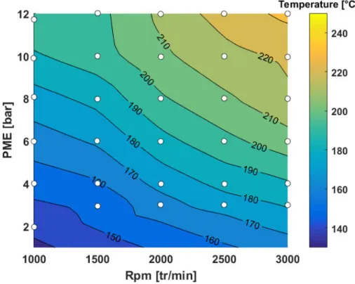
a cleaning process using fuel enriched in ethanol to clean the soot de-posit. The deposit includes a delay and reduces the sensitivity of the thermocouple. Such study hasn’t be done in the case presented here. . . 36 2.14 Map temperature for the piston. White circles: measured points. . . 37 2.15 Map temperature for the cylinder head. White circles: measured points. 38 2.16 Evolution of saturation temperature for n-heptane for different pressures
realistic of engine operating points. NIST database. . . 39 2.17 Timescale and experimental protocol visualisation for the influence of
piston impingement. . . 41 2.18 Simulation realised with IMPACT [29] (without aerodynamics) of the
effect of SOI on piston impingement. Top: ◦
CA of spray-piston impact. Bottom: Constant 90◦
CA. Set point 2000 rpm 10 bar BMEP. . . 41 2.19 Spray deflection simulation in an engine, cylinder wetting. . . 42 2.20 Evolution of piston surface temperature for the standard SOI. Set point
at 2000 rpm and a BMEP of 10 bar. . . 42 2.21 Temperature evolution at engine start and cylinder pressure evolution.
Engine speed ≈ 400 rpm. Top: full temporal evolution. Bottom left: first combustion cycle. Bottom right: Temperature differences established. 44
2.22 Effect of oil pressure on piston temperature. Switch from 2 to 4 bar is performed at t=60 s. . . 45 2.23 Evolution of piston temperature for two early injection timing. Left:
SOI -330◦
CA. Right: SOI -360◦
CA. Set point at 2000 rpm and a BMEP of 10 bar. The arrows highlight the impingement process. . . 46 2.24 PN generation for different SOI. Left: SOI steps and time evolution of
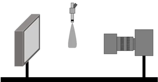
particle generation. Right: PN level as a function of the SOI. . . 48 3.1 Working principle of Shadowgraphy, the object observed is placed
be-tween a light source and the camera. . . 53 3.2 Two different histogramms showing how to achieve a 0.02 ms exposure
time. Top: Continuous light used with a ”fast” shutter. Bottom: Pulsed light used with a ”slow” shutter. . . 54 3.3 Close up shadowgraphy visualisation of 100 bar injection with two
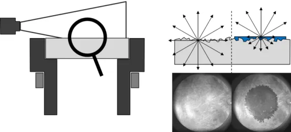
dif-ferent light sources. Left: Continuous LED panel. Right: Pulsed Laser. Courtesy of Continental . . . 55 3.4 GDI spray impinging upon a smooth plate. Fuel pressure is 100bar. . . 56 3.5 Sketch of the Refractive Index Matching experimental setup; a)
High-pressure pump b) GDI injector c) Plate holder d) Impinging plate e) Light source f) Heating collar g) Mirror h) High-Speed Video camera i) Computer. . . 56 3.6 Principle of RIM measurement. Left: Grazing Light illuminating a
trans-parent plate; Right: Modification of light path caused by wetting . . . . 57 3.7 Early injection process of n-heptane at 200bar, injection duration 5ms,
wall temperature 25◦
C . Left: Before spray impingement. Centre: Spray tip reaching the plate. Right: Secondary spray developing and starts of wetting. . . 58 3.8 Background subtracted images of secondary spray propagation during
injection process of n-heptane at 200bar, injection duration 5ms, wall temperature 25◦
LIST OF FIGURES
3.9 Steady state during injection process of n-heptane at 200bar, injection duration 5ms, wall temperature 25◦
C . Left: Mie scattering of the spray. Centre: Spreading phase. Right: Droplets reatomisation. Black arrows highlight the liquid film edge, yellow circle shows some droplets reatomi-sation. . . 59 3.10 Late injection process of n-heptane at 200bar, injection duration 5ms,
wall temperature 25◦
. Left: Late droplets reaching the plate (white area in the middle of the liquid film). Right: After injection process. . . 60 3.11 Calibration process of RIM method. . . 60 3.12 Calibration process for RIM measurement. Injection of 4µL of 20%
dodecane fuel. Top: Liquid film evolution. Left: Area evolution with respect to time. Right: Evolution of liquid film grey level. . . 62 3.13 Calibration curves for two different impingement angle . . . 63 3.14 Left: Boiling bubbles developing in the liquid film. Middle: Entrapped
bubbles during injection process. Right: Direct visualisation of liquid film surface soon after the end of injection. Arrows indicate bubbles. . . 65 3.15 RIM Alu set-up. Left: a) pressure pump b) GDI injector c)
High-pressure spray d) Aluminium plate e) Mirror f) Plate holder g) Light source h) High-Speed Video camera i) Camera. Right: Picture of the experimental set-up. . . 67 3.16 Visualisation of liquid film with RIM Alu method. Left: Raw image of
liquid film. Right: Background subtracted image of the liquid film. . . . 67 3.17 Top visualisation of impingement plates used to perform RIM methods. 68 3.18 Left: Top view of the instrumented plate with gold coating. Right: Side
view of the instrumented plate with apparent thermocouples. . . 68 3.19 Side cut of the thermo-instrumented plate. . . 69 3.20 Top view of the instrumented plate. . . 70 3.21 Left: Working principle of thermocouple. Right: Working principle of
zero degree compensation in the case of iron-constantan couple [19]. . . 70 3.22 Top Left: Overview of the amplification system, in green the backpanel,
in blue the amplification modules. Top Right: Break-out box. Bottom Left: Exit panel with BNC connections. Bottom Right: 5 V Power unit. 72 3.23 ETAS-ES 1000 used as acquisition surface for thermocouple signals. . . 73
3.24 Translation plate used to displace the thermocouple plate. Manual linear stage NEWPORT M-UMR 8.51. . . 73 3.25 Left: Positioning of optical pen for film thickness measurement. Right:
Measurement principle of confocal interferometric device. Here the de-vice measures the distance between a plate and a sample not the thick-ness of a liquid film (STIL-DUO user manual). . . 74 3.26 Two different visualisations of profiles sampled with AFM. Top: Zoom
on sapphire trough and crest. Bottom: Same horizontal and vertical scales. The thickness presented here, is a height variation in relatively to the position of the probe. . . 76 3.27 Translation and rotation plate allowing the correct positioning of the
injector. NEWPORT M-UMR12.63 and M-UTR120 material . . . 77 3.28 Left: Side vision of the impingement angle definition. Right: Top vision
of the impingement angle definition. . . 77 3.29 Goniometer set-up for the advancing and receding angles of n-decane on
a sapphire plate. . . 78 4.1 Images of a film spreading as visualized from bottom on the RIM setup.
Pi = 100 bar Ti = 6 ms and z = 50 mm. Images are displayed every
1.25 ms. . . 83 4.2 Time evolution of the liquid film area. Experimental conditions: Ti= 6
ms, Pi = 100 bar, z = 50 mm. The vertical dashed line indicates the
end of injection. . . 83 4.3 Evolution of digitation wavelength with respect to fuel pressure for Ti =
6ms and z = 50mm. The dashed line represent the power law Pi−1/3. . . 85 4.4 Detail of surface waves for different injection conditions for Ti = 10 ms
and z = 50 mm. Left to Right: 50, 100, 200 bar. . . 85 4.5 Evolution of film surface waves speed with respect to their radial position
r. Experimental conditions Pi = 100 bar, Ti = 10 ms and z = 50 mm.
The curves represent a r−1/2
evolution expected for a planar radial wave. 86 4.6 Liquid film area for different injection times. Experimental conditions
Pi = 100 bar and z = 50 mm. Continuous Line: Eq. 4.6, Dashed line:
LIST OF FIGURES
4.7 Liquid film area for different injection pressures. Experimental condi-tions Ti= 6 ms, z = 50 mm. (top) film at the end of the injection from
left to right for Pi=50, 100 and 200 bar. (bottom) Time evolution of the
film area. Continuous Line: Eq. 4.6. Dashed line: solution of Eq. 4.10. . 88 4.8 Liquid film area for different injector-wall distances. Experimental
con-ditions Ti= 6 ms, Pi = 100 bar. Continuous Line: Eq. 4.6, Dashed line:
solution of Eq. 4.10. . . 89 4.9 Sketch of the modeled problem. The film thickness is supposed to be
homogeneous. . . 89 4.10 Evolution of the film surface as a function of Pi1/3Q2/3η− 1/3t for all the
experiments presented above. Line: Equation 4.6 (see the text for the value of KP and Km) . . . 91
4.11 Evolution of the dimensionless area A∗
= (A − Ao)/(Ai− Ao) versus the
dimensionless time t/Ti for different injection durations and pressures. . 93
4.12 Impingement process of different fuel on sapphire plate. Ti = 6 ms,
Pi = 100 bar z = 50mm Tw = 20◦C. Top: n-heptane spreading. Bottom:
n-decane spreading. . . 95 4.13 Area evolution of n-heptane and n-decane. Injection conditions Ti = 6
ms, Pi= 100 bar z = 50mm Tw = 20◦C. . . 96
4.14 Impingement process on different roughnesses plate. Ti = 6 ms, Pi =
100 bar z = 50mm Tw = 20◦C. Top: Smooth sapphire plate. Bottom:
Ra= 20µm quartz plate . . . 97
4.15 Area evolution of n-decane on two different plate, a smooth sapphire plate and a rough Ra= 20µm quartz plate. Injection conditions Ti = 6
ms, Pi= 100 bar z = 50mm Tw = 70◦C. . . 98
4.16 Liquid film visualisation 5 ms after the end of injection. From left to right, 22◦ C, 70◦ C, 90◦ C, 120◦ C. Injection conditions, Ti = 6 ms, Pi = 100 bar. . . 101 4.17 Area evolution for different temperature (injector and wall temperature
set at the same level). Injection conditions, Ti = 6 ms, Pi = 100 bar.
For some temperature less measurement point are performed, when the measurement were done the focus was on the spreading phase and not on the relaxation phase. . . 101
4.18 Effect of viscosity on spreading rate. Comparison between experimental data and power law η−1/3
as presented by the spreading model. . . 102 4.19 Working principle of the algorithm used to optimise Km. Where ∆A∗ =
A∗
(n + 1) − A∗
(n). . . 103 4.20 Dimensionless area of n-decane liquid film for different injection
dura-tion (2, 4, 6, 8, 10 and 12 ms), different injecdura-tion pressure (50, 100, 200 bar) and different temperatures (22◦
C, 70◦
C, 90◦
C, 120◦
C). Left: Before optimisation on the coefficient of mass deposition Km. Right:
After optimisation on the coefficient of mass deposition Km. Black line
represents y = x equation. . . 104 4.21 Effect of the algorithm on Km and the fuel temperature at impact. Left:
Evolution of the mass deposition coefficient Kmwith respect to injection
temperature. Right: Evolution of the temperature of the spray at im-pact versus its temperature at the nozzle exit. Black lines present some iterations of the model. Black dots present the converged values. . . 104 4.22 Image of film spreading of n-decane on a quartz plate, with an
impinge-ment angle of 60◦
. Pi= 100 bar, Ti= 6 ms and z = 50 mm. . . 106
4.23 Evolution of liquid film shape with respect to impingement angle at 6.5 ms after start of injection. Pi = 100 bar, Ti = 6 ms and z = 50 mm. . . 107
4.24 Time evolution of the liquid film area for several impingement angle. Experimental conditions: Ti = 6 ms, Pi = 100 bar, z = 50 mm. . . 108
4.25 Evolution of ellipse focus position on time averaged image, the white area in the centre is the impingement area. Red squares present the position of the focus through time. White line displays the edge of the liquid film at the end of injection. Impingement angle is 60◦
. . . 108 4.26 Visualisation of liquid film edges together with ellipse contour and axes
at a given time (5 ms after start of injection). Injection pressure Pi =100
bar, injection duration Ti =6.0 ms. . . 109
4.27 Description of the parameters of an ellipse. . . 109 4.28 Temporal evolution of ellipse descriptors (a + c) and (a − c) parameters
for several angles. Pi = 100 bar, Ti = 6 ms. . . 111
4.29 Temporal evolution of ellipse descriptor p for several angles. Pi = 100
LIST OF FIGURES
4.30 Temporal evolution of the liquid film eccentricity for different impinge-ment angle. Injection pressure Pi =100 bar, injection duration Ti = 6
ms. . . 112 4.31 Eccentricity evolution for different impingement angle, together with the
fit proposed Equation 4.18. . . 113 4.32 Evolution of the spreading rate for the head (a + c)2 and back (a − c)2
of the liquid film, together with the fit proposed in Equation 4.19. . . . 113 4.33 Evolution of the spreading rate for the side p2of the liquid film, together
with the fit proposed Equation 4.19. . . 114 4.34 Liquid film visualisation on quartz plate at several time after start of
injection. Pi= 100 bar, Ti= 6 ms. . . 115
4.35 Average thickness evolution for three different impingement angles (90◦
, 60◦
and 45◦
) and pressures (50 bar, 100 bar, 200 bar). The mass injected is kept constant in all the injection scenario. . . 116 4.36 Area evolution for three different impingement angles (90◦
, 60◦
and 45◦
) and pressures (50 bar, 100 bar, 200 bar). The mass injected is kept con-stant in all the injection scenario. During the first ms the area is highly overestimated due to image detection algorithm that has difficulties to differentiate the liquid film and the sparse droplets. . . 116 4.37 Mass evolution for three different impingement angles (90◦
, 60◦
and 45◦
) and pressures (50 bar, 100 bar, 200 bar). The mass injected is kept constant in all the injection scenario. . . 117 5.1 Fast surface thermocouple measurement for n-heptane impingement.
In-jection duration 6 ms, inIn-jection pressure 100 bar, wall temperature 100◦
C , fuel temperature 30 ◦
C and injector to wall distance 50 mm. Left: Raw data with sample rate of 0.2 ms. Centre: Filtered data with 2 ms moving average. Right: Averaged measure over 10 repeats for the same injection conditions. . . 123
5.2 Fast surface thermocouple measurement for n-heptane impingement. In-jection duration 6 ms, inIn-jection pressure 100 bar, wall temperature 100◦
C, fuel temperature 30 ◦
C and injector to wall distance 50 mm. Left: Physical description during the impact. Right: Temperature evo-lution focussed on the heating phase. . . 124 5.3 Simultaneous temperature variation of the four thermocouples, for an
impingement angle of 60◦
. Wall temperature is 100◦
C , fuel temperature is 30◦
C , injector-wall distance is 50 mm and injection pressure and duration are 100 bar and 2.12 ms. . . 126 5.4 Temperature map for orthogonal impingement. Wall temperature is
100◦
C, fuel temperature is 50◦
C, injector-wall distance is 50 mm and injection pressure and duration are 100 bar and 6 ms. . . 127 5.5 Temperature profile generated by orthogonal impingement. Continuous
and dashed line are the same data mirrored to asses symmetry of the profile. Same conditions as Figure 5.4. . . 127 5.6 2D Temperature map for 60◦
impingement angle, injection duration 6 ms, fuel temperature 30◦
C, injection pressure 100 bar Left: Wall tem-perature 100◦
C. Right: Wall temperature 150◦
C. . . 128 5.7 2D Temperature map for 45◦
impingement angle, injection duration 6 ms, fuel temperature 30◦
C , injection pressure 100 bar and wall temper-ature 100. . . 129 5.8 Effect of injection duration on wall cooling. Injection pressure 100 bar,
wall temperature 100◦
C, fuel temperature 30◦
C, injector to wall distance 50 mm. . . 131 5.9 Effect of injection pressure. Wall temperature 100◦
C, fuel temperature 30◦
C, injection duration variable (i.e. constant mass), injector to wall distance 30 mm. . . 133 5.10 Effect of wall temperature, fuel temperature 30◦
C. Left: injection pres-sure Pi = 50 bar, injection duration Ti = 3.0 ms. Right: injection
pressure Pi= 200 bar, injection duration Ti= 1.5 ms . . . 133
5.11 Nucleate boiling on the thermocouple for injection temperature of 150◦
C. Left: nucleation site attached. Right: thermocouple visible without nu-cleation. Arrow and circle highlight the thermocouple position. . . 134
LIST OF FIGURES
5.12 Effect of fuel temperature. Wall temperature 100◦
C , injection pressure
Pi = 100 bar, injection duration Ti= 6.0 ms . . . 135
5.13 Effect of spray travelling distance, wall temperature 150◦ C , fuel tem-perature 30 ◦ C and injection pressure Pi = 100 bar, injection duration Ti= 2.12 ms. . . 136
5.14 Heat flux and temperature temporal variation. . . 139
5.15 Heat transfer coefficient variation [89] . . . 139
5.16 Heat flux calculation of Arcoumanis [2] and Meingast [56]. . . 140
5.17 Heat flux and temperature temporal variation experiment vs model. Dashed line presents the model and plain lines presents the experimental data. Injection condition Pi = 100 bar, Tw = 100◦C and fuel tempera-ture is 30◦ C. . . 142
5.18 Proposed shape for the heat transfer coefficient. . . 143
5.19 Evolution of heat flux and wall temperature for variable injection dura-tion. Dashed line present the model, plain line the experimental data. For sake of clarity experimental data are not shown on the flux curve. Injection condition Pi = 100 bar, Tw = 100◦C and fuel temperature is 30◦ C. . . 143
5.20 Evolution of the heat transfer coefficient h for different injection dura-tion. Injection condition Pi = 100 bar, Tw = 100◦C and fuel temperature is 30◦ C. . . 144
6.1 Summary of state of the art in terms of cooling regimes [7]. . . 146
6.2 Simulation of streamlines inside a bubble flowing through gas by Chiang et al.[13]. . . 148
6.3 Heat flux evolution and droplet lifetime curve with respect to wall tem-perature. Case of gently deposited droplets, TCHF = Tnuk [59]. . . 149
6.4 Overview of droplet global representations of the impact regimes and transition conditions for a dry heated wall. (a) Bai and Gosman [4]; (b) Rein [76]; (c) Lee and Ryu [48]. As presented in [59]. . . 150
6.5 Images of Injector coking: Right [36] Cleaned, fouled and cleaned up injector. Left [30] SEM image of a coked injector hole . . . 152
6.6 Distillation curve for 91AI fuel, 91AI fuel + 10% methanol, 91AI fuel + 15% methanol [9] . . . 153 6.7 Composition of AI91 gasoline from [9] . . . 154 6.8 Fuel film thickness evolution. Left: hexane liquid film with Tw = 23◦C.
Right: heptane liquid film with Tw = 30◦C. Dashed line illustrate the
identified linear behaviour of the film thickness evaporation. . . 156 6.9 Fuel film thickness evolution. Left: iso-octane liquid film with Tw =
23◦
C. Right: decane liquid film with Tw = 50◦C. Dashed line illustrate
the identified linear behaviour of the film thickness evaporation. . . 156 6.10 Schematic vision of STIL measurements. The arrows present possible
positions for the measurement in case of nucleate boiling. Position a: no problem encountered. Position b: thickness might be underestimated because of the bubble presence. Position c: too many interfaces to perform a correct measurement. Position d: the surface curvature makes the measurement impossible. . . 157 6.11 Fuel film thickness evolution. hexane/iso-octane liquid film with Tw =
23◦
C . Dashed line presents the vaporisation rate of single components superimposed in order to compare mono- and multi-components vapor-isation behaviours. . . 158 6.12 Area evolution for Surrogate 2 fuel film injected on Aluminium plate.
Left: Wall temperature Tw=80◦C. Right: Injection pressure Pi= 100 bar.159
6.13 Thickness evolution for surrogate 2 and 3 for a wall temperature Tw =
80◦
C. Left: injection pressure Pi= 30 bar. Right: injection pressure Pi=
100 bar. . . 160 6.14 Liquid film evolution for orthogonal impingement. Wall temperature
Tw = 150◦C, injection temperature TF U = 150◦C, injection duration
Ti= 6.00 ms and injection pressure Pi= 100 bar. . . 161
6.15 Liquid film evolution for orthogonal impingement. Wall temperature Tw = 180◦C, injection temperature TF U = 180◦C, injection duration
Ti= 6.00 ms and injection pressure Pi= 100 bar. . . 162
6.16 Liquid film evolution for orthogonal impingement. Wall temperature Tw = 210◦C, injection temperature TF U = 180◦C, injection duration
LIST OF FIGURES
6.17 Zoomed visualisation of a n-decane film 15 ms after the start of injection for different plate temperature. Injection duration Ti = 6.00 ms and
injection pressure Pi = 100 bar. . . 163
6.18 Aluminium plate mimicking a bowl shape. Length 3.5 cm, width 3 cm, height 1 cm (between bottom and top of the bowl). . . 164 6.19 Shadowgraphy of spray impinging on a hot wall, bowl shape geometry.
Wall temperature Tw = 130◦C, injection duration Ti = 2.12 ms and
injection pressure Pi = 100 bar. . . 164
6.20 Shadowgraphy of spray impinging on a hot wall, bowl shape geometry. Wall temperature Tw = 200◦C, injection duration Ti = 2.12 ms and
injection pressure Pi = 100 bar. . . 165
8.1 Coked piston visualisation together with the roughness measurements performed on a coked zone. Top: piston visualisation. Centre: roughness measurement in the non coked zone. Bottom: roughness measurement in the coked zone . . . 172
List of Tables
1.1 Evolution of emission regulations in Europe. CO: Carbon monoxide, NOx: Nitrogen oxides, PM: Particulate Matter, PN: Particle Number. 2 1.2 Characteristics of the injectors used in this study. . . 8 1.3 Notable dimensionless numbers for the study of impacting droplets. A,
a and b are constant that differs between the model and experimental facilities which helped defining the splashing criterion. . . 17 1.4 Splashing ratio in number and mass computed from the PDA
analy-sis performed on ASTRIDE injector. Adhered mass regroups sticking, spreading and half of splashing droplets. Whereas, away mass corre-spond to rebounding and half of splashing droplets. . . 18 2.1 Characteristic temperature for selected alkanes for gently deposited droplet
as depicted in [24] at atmospheric pressure. . . 38 2.2 Oil pressure test results. ∆T is the difference of temperature recorded
when switching the oil pressure from 2 to 4 bar. . . 45 2.3 Temperature loss on thermocouple 2 due to spray impingement on the
piston, extracted from Figure 2.23. . . 46 3.1 Amplitude parameter of plate roughness used in the different
experimen-tal methods. The arithmetical mean deviation Ra, the profile root mean
square Rq, the maximum peak height Rp, the maximum valley depth
Rv and the maximum height of the profile Rt are common description
parameters used to characterise surface roughness. . . 63 3.2 Optical pen measurement characteristics. STIL S.A. . . 74
3.3 Roughness parameters obtained with an AFM microscope on the sap-phire plate . . . 75 4.1 Value of the parameter C for different pressures of injection and injection
durations. . . 94 4.2 Spreading differences between n-heptane and n-decane in the same
ex-perimental conditions. . . 96 4.3 Spreading differences between smooth and rough plate in the same
ex-perimental conditions. . . 99 4.4 Selected n-Decane properties at variable temperature. . . 100 4.5 Overview of the experimental campaigns performed on film spreading
topics. . . 119 5.1 Effect of injection duration on wall cooling. . . 132 6.1 Properties of Surrogate n◦ 1 at 20◦ C . . . 153 6.2 Properties of Surrogate n◦ 2 at 20◦ C . . . 154 6.3 Properties of Surrogate n◦ 3 at 20◦ C . . . 155 6.4 Summary of vaporisation rate for Alcanes [µm/s] . . . 157
Nomenclature
α Thermal diffusivity ¨
R Temporal derivative of ˙R ∆P Pressure driving the liquid film
∆T Temperature variation from the set-point ˙
m Mass flow rate ˙
R Temporal derivative of R ǫ Ellipse eccentricity η Efficiency of the cycle η Liquid dynamic viscosity ηl Liquid dynamic viscosity
ηw Wall correction for viscosity
γ Heat capacity ratio
Γimpact Jet cross section at the impact
Γinjecteur Jet cross section at the injector exit
λ Digitation wavelenght
λ Thermal conductivity of the materia ν Liquid kinematic viscosity
Ω Liquid film volume
Ωi Liquid film volume at the end of injection
ρa The discharge gas density
ρf Fluid density
τ Dimensionless time θ Impingement angle
θ Temperature deficit of the surface θa Advancing angle
θr Receding angle
ϕ0 Intensity of the constant heat flux
ξ Dimensionless distance
◦
CA Degree cranck angle A Area of the liquid film a Major semi axis of the ellipse A∗
Dimensionless area
Ai Liquid film area at the end of injection
Ao Area of impact
Ao Area of the hole
B Background grey level
b Minor semi axis of the ellipse C Relaxation parameter
NOMENCLATURE
Ca Area coefficient
CD Discharge coefficient
Cv Velocity coefficient
d Droplet diameter
Do Outlet diameter of the nozzle
e Thickness of the liquid film F Focus of the ellipse
h Heat transfer coefficient I Raw image grey level K Splashing parameter
Kη Coefficient of wall correction for viscosity
Km Coefficient of mass
KP Pressure transfer function
Mdep Mass deposited on the wall
Mimp Mass impacted
Minj Mass injected
MsecS Mass participating to the secondary spray
p Semi-latus rectum of the ellipse Pi Injection pressure
Q Injection discharge of the injector q′′
w Heat flux density
r Compression rate
r Radial distance from the center of the liquid film Ra Arithmetical mean roughness
Re Reynolds Number
Ri Liquid film radius at the end of injection
Ro Radius of impingement area
Rp Maximum peak height
Rq Profile root mean square
Rt Maximum height of the profile
Rv Maximum valley height
S Spray penetration T Temperature Tf Fuel temperature Ti Injection duration Tw Wall temperature TF U Injector temperature
Tinit Wall temperature at the set-point
TLei Leidenfrost temperature
TN uk Nukiyama temperature
Tsat Saturation temperature
V Liquid film velocity v Dimensionless grey level
NOMENCLATURE
vb Liquid film velocity towards the backward direction
vf Liquid film velocity towards the frontward direction
vs Liquid film velocity towards the side direction
We Webber Number
z Injector to wall distance AFM Atomic Force Microscope
AI50 Integrated area with 50% of heat release APC AVL Particle Counter
BMEP Break Mean Efficiency Pressure CFD Computational Fluid Dynamics
CMOS Complementary Metal Oxide semi-Conductor CO Carbon Monoxide
ECU Electronic Control Unit GDI Gasoline Direct Injection LIF Laser Induced Fluorescence NEDC New European Driving Cycle NOx Nitrogen Oxides
OEM Gasoline Direct Injection
PAH Polycyclic Aromatics Hydrocarbons PID Proportional integral derivative PM Particulate Matter
RIM Refractive Index Matching
SAWLI Spectroscopic Analysis of White Light Interferogram SCR Selective Catalyst Reduction
SOI Start Of Injection TDC Top Dead Center
1
Introduction
1.1
General Context
The year 1958 held the first World Forum for Harmonisation of Vehicle Regulations. The purpose was to define some rules that would apply in all the signatory countries for the road vehicles. It gave some regulations on a lot of subjects such as safety, durability, environmental protection, energy efficiency, etc... In 1970, a first driving cycle has been defined, it is supposedly representative of the use of personal cars in Europe in an urban cycle. In 1990, they extended the driving cycle to extra urban cycles and in 1993, the Euro 1 standard for emission was created. Nowadays, the Euro 6d-TEMP is in use. In the mean time, different standards were created all over the world in order to meet the requirements of customers behaviours.
Table 1.1 shows the evolution of regulations for medium passenger cars in Europe. It appears that Carbon monoxide (CO) and Nitrogen oxides (NOx) emissions regulations have been reduced by almost three in 22 years. Regulations on NOx were introduced in 2001 and in 2011, the regulations on particle emissions were started. These standards need to be fulfilled during homologation cycles, which aim at being relevant of the normal use of a passenger car. The cycle itself is at least as important as the emission regulation. In Europe, from 1973 to 2018, the New European Driving Cycle (NEDC) was used (updated in 1996). It has been replaced in 2017 and 2018 by the Worldwide harmonised Light vehicles Test Procedures (WLTP) which is supposed to be more representative of real driving experience.
Name Year CO [g/km] NOx [g/km] PM [g/km] PN [#/km] Euro 1 1993 2.72 - - -Euro 2 1997 2.2 - - -Euro 3 2001 2.3 0.15 - -Euro 4 2006 1 0.08 - -Euro 5 2011 1 0.06 0.005 6.0 1011 Euro 6 2015 1 0.06 0.0045 6.0 1011
Table 1.1: Evolution of emission regulations in Europe. CO: Carbon monoxide, NOx: Nitrogen oxides, PM: Particulate Matter, PN: Particle Number.
In the late 2000’s and the early 2010’s, together with these type approval legislations, the necessity to decrease the fleet average CO2 emissions lead the manufacturers to
decrease the fuel consumption, and hence to reduce the engines size. The objective was to increase the power/volume ratio of the engine in order to maintain car power while reducing the consumption and emissions. To achieve these requirements, turbo-compressor and direct injection of gasoline were mainly used. Both elements help increasing the quantity of air admitted in the same volume, allowing to inject more fuel and hence increase the power produced during combustion. The turbocharger, by forcing more gases to enter in the combustion chamber, and the direct injection by cooling the admitted air thanks to fuel droplet vaporisation (the density of cold gases is higher than hot gases) .
However, the use of direct injection for gasoline engines also raised a new issue. Though gasoline engines were already producing particles, the use of direct injection increased significantly the particle level either PM or PN (mainly because of the ap-parition of liquid films and a worse mixture than in port-fuel injection engines, hence combustion inhomogeneities [42], Figure 1.2). Liquid films, in this context, are thin liquid deposit created by the injection process. It can either be because of the impact of fuel spray on the walls of the combustion chamber, or liquid deposited on the tip of the injector while the injector’s needle is closing. Since these liquid film, were quickly identified as a source of pollutants, a great care has been taken to improve the injec-tion process. Several axes of ameliorainjec-tion can be tackled. In [47], the discussion is addressed.
1.1 General Context
Figure 1.1: Endoscopic visualisation of direct injection and combustion inho-mogeneities (probably soot luminescence or pool fires) [44].
Increasing the injection pressure allows to reduce the emission of particle number (PN). In [81], the reduction of particles is explained by a better air entrainment and a greater atomisation due to higher injection pressure. Therefore, it both implies a faster vaporisation and a better air/fuel mixing. It also allows to reduce tip wetting as mentioned in [16, 73]. Minimising tip wetting with the injector design is another way of improving the injection process, during the injection and specially at the end of injection. The purge of the injector promotes the apparition of liquid film on the injector tip [28]. It has been proven [70] that modifying the geometry of injector tip and/or holes can reduce significantly the tip wetting and consequently the particle generation due to this source.
Figure 1.2: Visualisation of the tip wetting, during the injector purge (i.e. after the needle closure) [28]. Black lines highlight the area of liquid deposition.
Tip wetting is also responsible for injector fouling (carbon deposit on the injector surface Figure 1.3 presented in [30]). The carbon deposit is responsible of higher spray penetration (by slightly changing the geometry of the holes), increasing the wall
im-pingement likelihood. It is also creating a porous media on the tip, where fuel gets entrapped and must lead to diffusion flame attached on the injector, the fouling of the injector can multiply the PN emissions by 100 [30].
Figure 1.3: Injector fooling due to tip wetting, carbon deposit slightly changes the hole geometry [30].
Finally, the injector coking can be cleaned using fuels with additives [57]. This leads to the last point addressed in [47] which is the fuel itself. Indeed the combustion of Polycyclic Aromatics Hydrocarbons (PAH) is responsible of soot formation [20, 23]. Hence, the fuel composition can be responsible for a higher or hopefully a lower particle generation. In [17] they tested the influence of the addition of butanol to gasoline on the engine emissions and specific consumption.
An aspect not addressed in [47] is the injection timing. Indeed the injection timing is crucial in direct injection engines. Most of particles are created during the com-bustion process: the air/fuel mixture is especially primordial. Particles are generated if inhomogeneities in the mixture are experienced: the rich zones (fuel/air ratio > 1 [74]) are of great concern [68] and they essentially occur next to liquid films, or if the turbulent flow does not have the time to correctly mix the gases. In [40], the timing of injection is studied in a 4 cylinder direct injection engine. Figure 1.4 shows how the particles number varies with the Start Of Injection (SOI). When the injection is too early (zone A), the spray impacts on the piston, creating a liquid film on the piston and, sometimes the cylinder head (due to splashing). The fuel vaporisation is too slow, and homogeneous mixture is not reached, leading to particle generation. When the start of injection is later (zone B), the fuel has a clear path, exchanges with the fresh gases are maximum, hence a good mixture is achieved and particle generation is really small. In zone C the conditions are relatively similar to zone B, however the time available for vaporisation is shorter, and the turbulence has decayed. A poorer mixture is achieved
1.1 General Context
and particle level starts to raise. Between zones C and D where the engine cannot lit, the mixture which is too inhomogeneous for the ignition to generate a viable flame. Fi-nally, in zone D, thanks to the piston geometry, a combustible mixture is present next to the spark plug and a stratified combustion occurs. Though ignition is performed, the combustion quality is poor and a lot of particles are produced.
Figure 1.4: Particle Number (PN) as a function of SOI and injection geometry [40].
It now appears clearly that, in direct injection engines, taking care of the injection process is fundamental for the reduction of emissions. Hence, a closer look to the injection and the impingement process is necessary. Downsized engines which are (as mentioned before) very popular for gasoline cars, have a typical volume of 1 to 1.2 litres with 2, 3 or 4 cylinders. A one litre engine with three cylinders, gives three combustion chambers with a swept volume of 0.33 litre (which is quite small, as big as a soda can). Typical dimensions for the bore (cylinder diameter) is around 70 mm and the stroke (height travelled by the piston during one stroke) is around 80 mm. Injection is performed in this small volume by high-pressure injectors at pressures up to 350 bar or even more (500 bar applications are coming). Droplet ejection velocity is ≃ 100 − 300 m.s−1
to affirm that spray-wall impingement will occur at some point in the engine map. Many different impingement configurations might be encountered, they depend mainly of the injector position and of the combustion chamber geometry. Figure 1.5 shows the two common configurations for the position of the injector (central and side), it also highlights the variability of impingement angles (between the spray plumes and the wall impacted wall). Last but not least, the impingement of sprays on walls is not
Figure 1.5: Common position for the injector. Left: Central Mounted. Right: Side Mounted. Highlights the variability of impingement angle encountered in a Direct Injection (DI) engine.
only encountered in direct injection engines. It is important to keep this in mind, as the worldwide trend is to reduce the development of high power fuel engines and replace it with electrical or hybrid engines. Though, fuel impingement also happens in port fuel engines (fuel is injected in the intake pipes and mixed air/fuel is admitted in the combustion chamber). In Selective Catalyst Reduction (SCR), urea is injected with modified port-fuel injectors in the catalyst system in order to reduce NOx emissions at the exhaust. SCR systems are also facing liquid films issues, which sometimes lead to solid by-product deposits and strongly deteriorate the system. Finally, non automotive applications can be found, specially for cooling systems as the heat removal of sprays is really important. The heat transfer of sprays will be addressed in Chapters 5 and 6.
1.2 About injection process and engine working
1.2
About injection process and engine working
In the context of emission reduction, which is a worldwide concern, the injection process and specially the liquid film formation have been identified as major concerns. The objective of this PhD book is to improve the knowledge about fuel film generation, spreading and vaporisation. To do so, a closer look at the injection process is done.
To perform a correct injection, three main components are necessary: an injector, a fuel pump and an Electronic Control Unit (ECU). These three components are built by automotive suppliers. Continental is producing the three components in order to provide to car manufacturers an injection solution (Figure 1.6).
Figure 1.6: High pressure injector, ECU and high pressure pump
pro-duced by Continental. (Courtesy of Continental website
www.continental-automotive.com)
The principal requirement (before looking at the emissions), is to inject the correct quantity of fuel to produce the power required by the driver at the required time. The ECU is in charge of triggering and powering the injector, it is previously calibrated to make sure the fuel request is in accordance with the power required by the car. Another requirement for Continental is to produce injectors with high reliability, as the injection process is performed thousands of time each minute. Finally, the targeting (spatial position of injectors plumes) of the injection needs to be elaborated, to satisfy the specificity of the engine in which the injector is placed.
The injector used in the following study has the following characteristics (Table 1.2). It is an experimental three-holes injector, developed on the body of the classical five or six-hole injectors of its generation (commercialised by Continental). It has been developed for the ANR-ASTRIDE [1]. The reason to use a three-hole injector is because it is much simpler to study. Indeed, while looking at a single plume the two others are
not likely to disturb the visualisation. A five-hole injector described in Table 1.2 is the one used in the engines measurements presented in Chapter 2. It is only used in this chapter, for all the other measurements the ASTRIDE injector is used.
Injector Holes Mass Flow Rate
[g/s] @100 bar Sauter Mean Diameter [µm] @100 bar Hole Diameter [mm] ASTRIDE 3 6.5 15.1 @ 75 mm 0.2 Serial 5 7.35 9.7 @ 50 mm 0.18
Table 1.2: Characteristics of the injectors used in this study.
As mentioned before, the injection of the correct quantity of fuel amount is necessary in order to perform a good stoichiometric combustion. However, it is also necessary to have a homogeneous mixture between air and vaporised fuel. It is therefore mandatory to give enough time to the fuel to vaporise. Consequently, a temporal window for injection can be defined to indicate when injection should happen and when it should not. The working principle of a gasoline engine is to chain combustion cycles in order to rotate a crankshaft which transmits power to the wheels (very simplified vision). During each combustion cycle, fuel is burned and pushes a piston, the combustion cycle is composed of four strokes depicted Figure 1.7 (the four strokes give its name to the four stroke engine, broadly used in automotive engines). To complete the four strokes, two complete rotations of the crankshaft are necessary, an engine running at 2000 rpm will then complete 1000 combustion cycles by minute and by cylinder. The four strokes are [31]:
• The Intake: during this phase, the intake valves are opened and the piston is going downward. It creates an aspiration of the fresh gases, introducing the necessary amount of oxygen in the combustion chamber. Generally the injection of fuel starts during the intake.
• The Compression: during compression, the intake valves are closed and the piston is going upward. The pressure of the chamber increases, and the fuel is vapor-ising and mixed thanks to the air motion generated by the combustion chamber geometry.
1.2 About injection process and engine working
• The Power: at the very end of the compression, the spark plug fires so the com-bustion of the air/fuel mixture starts at the beginning of the power stroke. The expansion of gases during the combustion generates a force that pushes the piston downward, and will give power to the wheels.
• The Exhaust: here, the piston is going upwards, and the exhaust valves are open. It sweeps most of the burned gases out of the combustion chamber. A new combustion cycle can start.
Figure 1.7: Schematisation of the four strokes of a gasoline engine. Intake, Compression, Power and Exhaust. The spark usually takes place at the very end of compression however for sake of clarity it is represented during the
power stroke. Every stroke takes 180◦CA (Crank angle).
Though the combustion takes place during the third stroke, it is the two first strokes that are primordial to achieve a good and clean combustion. As the injection, fuel vaporisation and air fuel mixing needs to be performed during these two strokes. In order to fix the figures for the reader, let us take an engine running at 2000 rpm (typical engine speed for a gasoline engine). The intake and compression takes one rotation of the engine, that is to say 30 ms. A typical injection duration is 1 to 8 ms depending on the load of the engine, the injector mass flow rate, and the injection pressure. As the impingement of the piston should be avoided, the injection generally starts after 50 − 70◦
of crank rotation, which is 5 ms, hence it only leaves 25 ms to complete injection, vaporisation and mixture. That is to say 20 ms for vaporisation and mixture, this is most of the time enough and particle generation are kept low.
However, and this is why the study of injection process and liquid film is important, in some cases, the time available is not long enough. At the engine start, after decelerating or while strongly accelerating (power is no longer needed so the engine cools down), the engine is relatively cold and vaporisation is deteriorated. Also, between two operating points, the inputs of the engine are changing really fast (injection duration, engine speed etc...) however it takes some time for the boundary conditions (piston and cylinder temperature) to follows the set point. Hence, it creates transient points which are likely to generate particles.
The injection problem is a very complex tasks, and calibration of injectors on engine map is a huge amount of work. For every engine, several people are working full time to develop injection strategies. The strategies should optimise the injection in term of fuel consumption while minimising pollutant generation (in some extreme cases, it should make sure the cylinder will just fire correctly). Now that the injection process has been addressed as a frame for the study, a zoom at the injector scale and specially on the impingement process is proposed.
1.3
Dynamic of droplets and spray impingement
1.3.1 Injector and spray description
Table 1.2 shows an insight of the injector characteristics. However, a full description of the spray produced by the injector is presented here as it is the cornerstone of all the studies presented later. As mentioned before, the injector is a three-hole solenoid injector, it has been specially developed for experimental studies. Performing direct visualisation of sprays or liquid films with 5 or 6 plumes is quite complicated. Two concrete examples are: i) when a plume is disturbing the background for shadowgraphy visualisation, ii) when the liquid films generated by two plumes are overlapping. Hence, having only three plumes was better for experimental research.
Figure 1.8 shows the penetration curves of the injector at 50, 100 and 200 bar. The observation window is limited to penetration smaller than 90 mm. It explains why the curve for 200 bar is completely flattened 1 ms after the start of injection. The penetration curve were made using backlit illumination (or shadowgraphy), the method is presented in Section 3.2. A delay is also visible at the beginning of the curves. The delay corresponds to the time between and the release of pressurised flow
1.3 Dynamic of droplets and spray impingement
in the air. During this period the ECU generates the signal for the injector opening and the opening of the needle are performed.
Figure 1.8: Spray penetration for 50, 100 and 200 bar for ASTRIDE injector, based on shadowgraphy pictures in atmospheric conditions. Errorbar display-ing the standard deviation of measurements based on 5 independent repeats.
The penetration curve of high pressure injectors have been broadly studied, for diesel and gasoline applications. In [65], Naber and Siebers studied the spray penetration and derived a model. They show that pray penetration can be split in two parts: at the beginning the penetration is linear in time. Later on the penetration is proportional to √
t. The reasons for this change of spray behaviour have been stressed and modelled in many research papers. Among them, is the evolution of droplet velocity with respect to the surrounding gas, which is then put in motion through momentum transfer (from the liquid to the gas). At the beginning, the penetration is linear and the droplets are much, still undergoing atomisation, faster than the gas. Afterwards, droplets and gas are moving at the same velocity and the penetration becomes proportional to√t. Some mathematical models for high pressure spray penetration are proposed in [72, 83]. The model presented by Payri in [72] defines the penetration of the spray S when t < tr as:
S(t) = Cv
s 2∆P
ρf
and when t ≥ tr: S(t) = C 0.5 v (2 Ca)0.25 (a tanθ/2)0.5 ρ −0.25 a ∆P0.25 D0.5o t0.5, (1.2) where tr= (2Ca) 0.5 Cv a tanθ/2 ρf Do (ρa ∆P )0.5 , (1.3)
where ∆P is the pressure difference between the fuel and the surrounding gas, Cv is
the velocity coefficient, Ca the area coefficient, ρf the fluid density, ρa the discharge
gas density, Do the outlet diameter and θ the spray angle. It is important to note from
these formulas that in the linear area the penetration is not influenced by the outlet diameter nor the gas density. Whereas in the√t zone the penetration is affected by the gas density and the nozzle outlet diameter. Finally, in both regions, the penetration is influenced by the injection pressure, though the influence is greater in the linear zone than in the fully developed zone.
Finally, some penetration curves can be found in literature to highlight these two different comportments. Figure 1.9 shows the penetration curves presented in [77] and [72], the two temporal behaviour presented earlier are clearly identifiable.
The penetration curve of the injector used to produce all the results presented bel-low (excepted for the engine measurements) has a relatively long linear behaviour, it favourites the wall impingement (which is the worst case scenario for engine applica-tions). Which is good in our case as the spray-wall impingement is at the core of the whole study.
In [53], the influence of pressure on the discharge coefficient CD = A m˙
o√2ρf∆P [71]
is tested (Figure 1.10). ˙m is the injector mass flow rate and Aothe hole area. It can be
seen that for the pressure range we are interested in (20 to 200 bar), the variation of CD is around 5% which is relatively small. Though the injector are not the same, their
comportment is really close and the experimental facility are the same. Consequently, it will be considered that the variation in CD for our injector is not a dominant parameter
to consider.
In 2015, Giaocomo Piccinni Leopardi performed two-components PDA measure-ments of the injector at Loughborough University. Selected results are presented here to give some more knowledge about the spray distribution. The data produced are in-jectorwise (and not spraywise, Figure 1.11), it means that the two components velocity
1.3 Dynamic of droplets and spray impingement
Figure 1.9: Top: Spray penetration, as a function of time at various ambient pressures (injection pressure 1350 bar) [77]. Bottom: Penetration curve and calculation of the penetration parameter [72].
are in the injector axis and orthogonally to this direction. Figure 1.12 shows a picture of the spray during the measurement and the velocity distribution on a point at 40 mm and 100 bar. These results are performed during the steady state of the injection, that is to say without the injection head or tail.
Figure 1.13 shows the calculated Reynolds and Weber (as defined in Table 1.3) num-ber for a measurement point in the spray. Both histograms follow a Weibull distribution
Figure 1.10: Evolution of mass flow rate and discharge coefficient for different injection pressure [53].
Figure 1.11: Description of injectorwise and spraywise directions.
(often referred as Rosin-Rammler in granulometrie).
1.3.2 Impact regime description
Now that the injector and the spray composition have been presented, a presentation of the droplets outcomes is given. The objective here is not to make a complete review of droplets impacting regimes (as the subject is widely studied, and reviews already exists) but to give the necessary information to the reader for the understanding of spray impingement. Indeed, the literature is quite exhaustive about single droplet impact dynamics in ambient conditions [59]. However, spray-wall impact literature is
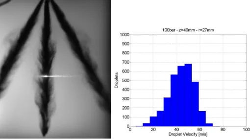
1.3 Dynamic of droplets and spray impingement
Figure 1.12: PDA measurement of the spray, and velocity distribution at 100 bar and 40mm.
Figure 1.13: Reynolds and Weber distribution at 100 bar, 40 mm away from the injector (See Table 1.3 for definition).
less detailed, because of the spray, the gas flow, the liquid film and the very numerous re-atomised droplets in the impingement zone which makes the study more complex [32, 37, 38].
The impact regimes for a droplet on a cold (relative to the saturation temperature of the liquid studied), flat, rigid and dry surface are generally separated in four different post-impingement scenarii (Figure 1.14). The details of a drop-wall impingement are very complex, especially when the impact energy of the droplet is high. Though, the
Figure 1.14: Post impingement scenario of single drop impact on cold, rigid and dry wall [5].
four scenarii (stick, rebound, spread and splash) introduced in [5] are most of the time valid:
• Stick: When the droplet is really slow, it may just stick to the surface and stop moving (thanks to contact forces).
• Rebound: As the impact energy increases, the air layer between the drop and the wall leads to a small energy loss and the drop rebounds.
• Spread: When the impact energy gets higher, the droplet is strongly deformed and can spread on the surface. The phenomenon is complex and a precise descrip-tion can be found in [3, 78]. As a competidescrip-tion between inertia and surface tension starts (dissipation via friction), a new equilibrium can be reached, depending on the surface wettability. At rest, a static contact angle can be defined between the liquid, the wall and the surrounding gas.
• Splash: If the impact energy gets even higher, the drop will disintegrate [3, 59, 63, 97, 101] as the inertial forces will overcome capillary effects. The splashing itself can take several forms such as prompt splash, corona splash, receding break-up, partial rebound, finger break-up [3]. A constant consequence of splashing is an atomisation process, the impacting droplets splits up. Depending on the scenario, some liquid (smaller drops) can stick or not on the surface.
The variety of droplets size, speed, composition (liquids) is really wide. Hence, dimensionless numbers are commonly used to describe drop-wall interactions. Consid-ering a droplet of diameter D, normal (to the wall) velocity U , specific mass ρ, viscosity µ and surface tension σ several dimensionless numbers can be defined. Here the focus is put on only three numbers, which are the Reynolds number Re, the Weber number
1.3 Dynamic of droplets and spray impingement
W e and the Splashing Criterion K defined in Table 1.3. The splashing criterion has been first introduced by Stow in 1981 [95], and then confirmed by Mundo in 1995 [63].
Dimensionless number Description Definition
Weber number Inertia / Surface tension W e =ρUσ2D
Reynolds number Inertia / Viscous forces Re = ρU Dµ Splashing parameter Defines a threshold
for splashing regime K = AW e
aReb
Table 1.3: Notable dimensionless numbers for the study of impacting droplets. A, a and b are constant that differs between the model and experimental facil-ities which helped defining the splashing criterion.
For a given droplet with a defined Reynolds and Weber numbers, the impact scenario can be evaluated. In [93, 94] Stanton and Rutland introduced two criterion for the stick/rebound limit and the rebound/spread limit. As these regime only concerns small and slow droplets, the Weber number value is sufficient to describe the impact outcome. For a Weber number W e ≤ 5 the droplet will stick to the wall and for a Weber 5 < W e ≤ 10 the droplet will rebound. The values presented here vary in literature depending on the experimental set-up, mainly because of surface tension, though, they give a good insight of the frontier (in term of Weber value) between stick and rebound. Finally the frontier between spreading and splashing is defined for droplets with a Weber W e > 10. If the Splashing parameter is below the splashing criterion the droplet will spread, if it is higher the droplet will splash. Studies give different values for the parameters A, a and b in the splashing parameter (defined in Table 1.3). As an example the values A = 1, a = 0.5, b = 0.25 and Kc = 57.7 were
identified by Mundo in [63] as reported in [25] and will be used in what follows. A summary of the different values for the parameters can be found in [59]. The problem described here, is for supposedly isolated droplets, impacting on dry walls. However
in the case of a spray impacting on a wall, some droplets are facing a dry wall and others a wetted wall. A splashing criterion for wetted surface are also available in [59], but is only valid for single droplets impacting on liquid films (sprays are even more complicated).
Table 1.4 presents, for different positions and pressures, the splashing ratio calcu-lated using the droplet distribution, pretending droplets are isocalcu-lated. It gives (with the previously defined criterion), between 40% and 80% of droplets (in number) in the splashing regime. These droplets are representing more than 80% in mass, of the spray droplets. Finally, taking as an hypothesis that, for a droplet in the splashing regime, 50% of the mass sticks to the wall and 50% is ejected away from the wall, it then gives that, more or less 50% of the mass impacting on the wall is deposited. This hypothesis is easily arguable, but it is inspired by the model adopted by Bai et al. [5]. Splashing to incident droplet mass ratio rm = msplash/mimp”is taken to have a random value evenly
distributed in the experimentally-observed range [0.2; 0.8] for a dry wall”. To have a rough idea of the mass deposited, fixing this ratio to 0.5 seems a fair hypothesis. The calculations presented here use strong hypothesis, as the objective is not to develop again a model of adhered mass using the droplets distributions. But to give to the reader a rough idea of what is happening when the spray is impacting on a plate.
In the definition of the Reynolds and Weber numbers, the velocity normal to the wall has been used. However, here the measurement has been performed in the direction of the injector as presented before. Hence, the deposition rate calculated correspond to piston impingement in a central mounted configuration (Figure 1.5).
Number ratio Mass ratio Mass Non-splash Splash Non-splash Splash Away Adhered 40 mm 100 bar 22.2% 77.8% 2.4% 97.6% 48.8% 51.2% 60 mm 100 bar 39.8% 60.2% 6.5% 93.4% 46.8% 53.2% 40 mm 200 bar 48.0% 52.0% 14.8% 85.2% 42.7% 57.3% 60 mm 200 bar 56.9% 43.11% 17.4% 82.6% 41.8% 58.1%
Table 1.4: Splashing ratio in number and mass computed from the PDA
analysis performed on ASTRIDE injector. Adhered mass regroups sticking, spreading and half of splashing droplets. Whereas, away mass correspond to rebounding and half of splashing droplets.
![Figure 1.9: Top: Spray penetration, as a function of time at various ambient pressures (injection pressure 1350 bar) [77]](https://thumb-eu.123doks.com/thumbv2/123doknet/2954030.80637/45.892.267.697.236.815/figure-penetration-function-various-ambient-pressures-injection-pressure.webp)
![Figure 2.15: Map temperature for the cylinder head. White circles: measured points. Fuel Saturation Temperature [ ◦ C] Nukiyama Temperature[ ◦ C] LeidenfrostTemperature[ ◦ C] n-heptane 98 150 210 iso-octane 99 122 190 n-decane 174 210 253](https://thumb-eu.123doks.com/thumbv2/123doknet/2954030.80637/70.892.180.651.231.606/temperature-cylinder-measured-saturation-temperature-nukiyama-temperature-leidenfrosttemperature.webp)