Prediction of macroscopic mechanical properties of a polycrystalline microbeam subjected to material uncertainties

(1)

ABSTRACT: The first resonance frequency is a key performance characteristic of MEMS vibrometers. In batch fabrication, this first resonance frequency can exhibit scatter owing to various sources of manufacturing variability involved in the fabrication process. The aim of this work is to develop a stochastic multiscale model for predicting the first resonance frequency of MEMS microbeams constituted of polycrystals while accounting for the uncertainties in the microstructure due to the grain orientations. At the finest scale, we model the microstructure of polycrystaline materials using a random Voronoï tessellation, each grain being assigned a random orientation. Then, we apply a computational homogenization procedure on statistical volume elements to obtain a stochastic characterization of the elasticity tensor at the second scale of interest, the meso-scale. In the future, using a stochastic finite element method, we will propagate these meso-scale uncertainties to the first resonance frequency at the coarser scale.

KEY WORDS: MEMS; Stochastic homogenization; Micro-beam resonance frequency.

1 INTRODUCTION

Microelectromechanical systems (MEMS) are microsystems made of at least one mechanical part. They are present in a wide variety of fields, including aeronautics, automobile, or medicine (e.g. heart catheter as blood pressure sensors) and their use is growing fast. Predicting precisely one or more mechanical properties is of major interest for some applications. However, a scatter between a predicted mechanical property and manufactured MEMS can be observed. This scatter results from the uncertainties involved in the manufacturing process.

These uncertainties can be of different natures. Two different MEMS will have different microstructures (grain sizes, grain orientations, surface profiles…). For a sufficiently large macroscopic scale, such randomness is negligible. However, for MEMS, the dimensions are comparable with the microstructure of materials. Thus the influence of the microstructure may not be negligible anymore.

The case study in this work is a clamped-free microbeam used for gyroscopes. For MEMS gyroscopes, structural dynamics may be of major importance. Interesting macroscopic quantities for designers are the resonance frequency of the first mode or the quality factor. The microbeam is made of polysilicon. As the properties of Silicon crystals are anisotropic, a first source of uncertainty is the grain orientation (other sources will be considered in a future work). The purpose of this work is the prediction of the macroscopic resonance frequency of the first mode of a microbeam from a random distribution of grain orientation at the microscopic scale.

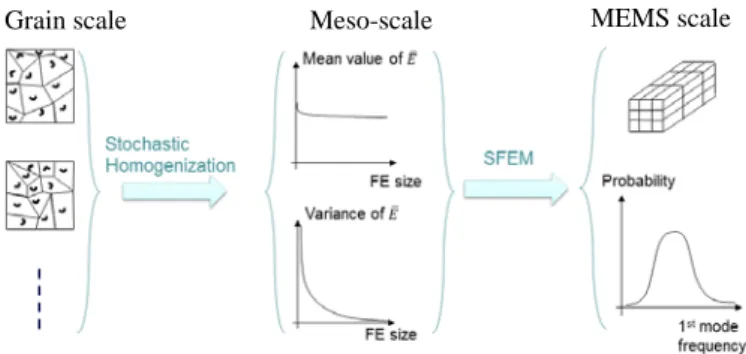
The resonance frequency can be predicted by using a 3-scale stochastic model. This is necessary since modeling each grain for the whole beam is computationally too heavy. The 3 scales are the following ones:

• The micro-scale or the grain scale is the smallest scale of this model. It models each grain with its particular elasticity tensor which depends on the orientation of the grain.

• The meso-scale is the intermediate scale. It is the scale over which the material properties of the grain are homogenized.

• The macro-scale is the whole microbeam over which the resonance frequency is sought, using homogenized material properties at the meso-scale.

The link between these 3 scales is depicted in Figure 1.

Figure 1- The 3-scale procedure

Samples of the microstructure can be generated with a random orientation for each silicon grain. They are referred to as the Statistical Volume Elements (SVE). A Monte-Carlo procedure along with a homogenization technique permits to estimate a distribution of the material properties at the meso-scale, as proposed in [1,2,3]. However computational homogenization is used here, based on [4,5,6] (see section 2.3) as it is more efficient although it requires the stiffness matrix of the microstructure. The support of the distribution can be bounded (from below and above) to match better the

Prediction of macroscopic mechanical properties of a polycrystalline microbeam

subjected to material uncertainties

Vincent Lucas1, Ling Wu1, Maarten Arnst1, Jean-Claude Golinval1, Stéphane Paquay2, Van-Dung Nguyen1, Ludovic Noels1

1

Department of Aeronautic and Mechanical Eng., University of Liege, Chemin des Chevreuils 1, B-4000 Liege, Belgium

2

Open-engineering SA, Rue des Chasseurs-Ardennais, B-4031 Liege(Angleur), Belgium email: vincent.lucas@ulg.ac.be

(2)

Proceedings of the 9th International Conference on Structural Dynamics, EURODYN 2014

observed behavior of the material. The bounds’ information can be added with the maximum entropy principle (MaxEnt) [7]. The final objective of this step is to be able to generate samples of the elasticity tensor that would mimic the microstructure randomness.

Once the distribution of the elasticity tensor is obtained at the meso-scale, the uncertainties can be propagated up to the macro-scale. A deterministic finite element method can be used in the frame of a Monte-Carlo procedure. Other methods can be considered to improve the computational efficiency. Polynomial chaos expansion can be considered [8], [9]. Stochastic Finite Element methods exist, such as spectral stochastic finite element [10]. The Perturbation approach can also be used. It gives a solution at a low computational cost, even though it may lack accuracy [11], [12], [13]. Finally, the Perturbation Stochastic Finite Element Method (PSFEM) considers a Taylor expansion around the mean to determine the output distribution. This meso-macro procedure will be investigated in the future.

The sections that follow focus on the microscopic part. The material, polysilicon, is first described. The homogenization procedure is then discussed. The last section derives the distribution of the material property at an intermediate scale: the meso-scale. From samples of the microstructure, distributions of the homogenized property can be constructed.

2 THE MICROSCOPIC PART

2.1 Silicon

Silicon is the most common material in microelectromechanical systems. It is an aggregate of cubic crystalline materials. The properties of a silicon grain depend on its orientation with respect to the crystal lattice. What follows here is based on [14]. The notation represents a plane with the integers , , and being the Miller indices. represents a direction (in the basis of the direct lattice vectors).

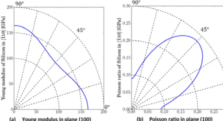
In the 100 , 010 and 001 directions, the same Young modulus is seen: 130 GPa, the minimum value for silicon. The maximum value of the Young modulus is obtained in the

111 direction: 188 GPa. The range of possible values for Poisson’s ratio is between 0.048 and 0.40. The behavior of the Young modulus and the Poisson ratio is depicted in Figure 2 in the plane 100 .

Figure 2 - Silicon material properties based on [14] Based on [14], which uses Hall measurements [15], Table 1 contains the different properties of Silicon. The , and

axes are aligned with the 100 , 010 and 001 directions. stands for the Young modulus while and correspond respectively to the Poisson ratio and the shear modulus. The parameters are the , elements of the matrix Voigt notation of the fourth order elasticity tensor .

Table 1. Measured mechanical properties Parameter Hall meas.

[GPa] 130 [-] 0.28 [GPa] 79.6 [GPa] 165.6 [GPa] 63.9 [GPa] 79.5 2.2 Homogenization: overview

Let us consider the micro to meso part: the homogenization of a volume element of the microbeam is sought. A portion of the material taken into consideration can be named a volume element. An example of a FE model, obtained with gmsh, can be seen in Figure 3. When this volume is large enough to have accurate, deterministic homogenization, it is called a representative volume element (RVE). The material properties can be extracted by applying suitable boundary conditions on the FE model. The Hill-Mandel condition must be verified [4,5,6] as it will be discussed later on. The homogenized computed property is called effective and does not depend on the boundary condition. If the volume element is too small to be representative, the homogenization possesses a random nature. It is a statistical volume element (SVE). The homogenized computed property is called apparent. The apparent properties of a SVE depend on the boundary condition.

Figure 3 - A sample of the microstructure

At first, let us consider a RVE. The volume average of over the volume is defined as

1 V

The subscript will refer to the microstructure while the subscript will refer to the homogenized case over the volume element. and Γ are respectively the volume and boundary while is the position vector. An effective elasticity tensor can be defined over an RVE. As said earlier, it is independent of the boundary conditions and thus unique for elastic material. can be defined through the relationship between the averaged stress tensor and the averaged strain tensor [16]:

(3)

: (1) If is the fluctuation of around its volume average

, then the following can be written ([16]):

: : :

Thus usually differs from . The latter is the approximate solution proposed by Voigt: the homogenized elasticity tensor is approximated by its average local value. As said by Hill, that solution is an upper bound for . It is named the Hill-Voigt bound.

The same reasoning can be done with the compliance tensor. is then a lower bound for the effective elasticity tensor. It is named the Hill-Reuss bound.

Bounds will be important in this section. How can we define ordering between 2 tensors? A tensor is (strictly) greater than a tensor if their difference is positive semidefinite (positive definite).

iif is positive (semi)definite Let us define the boundary conditions that respect the Hill-Mandel principle:

• Kinematic Uniform Boundary Condition (KUBC) • Static Uniform Boundary Condition (SUBC) • Mixed Boundary Condition (MBC)

• Periodic Boundary Condition (PBC)

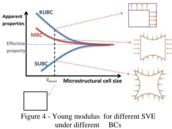
The independence of an RVE with respect to the boundary condition, when performing homogenization, can be used to define the concept of RVE. A volume element is said to be representative when the homogenized values obtained with KUBC and SUBC coincide [5]. If it is not the case, the volume element is too small to be representative and is stated statistical (SVE). KUBC and SUBC are two extreme boundary conditions (BC).

While the mixed and the periodic cases are estimates of the effective elasticity tensor, the uniform displacement (KUBC) overestimates the elasticity tensor while the static uniform BC underestimates it. For a SVE, the KUBC solution is an upper bound for the elasticity tensor while the SUBC case is a lower bound. A range of elasticity tensors is possible and one may talk about apparent properties. This can be seen in Figure 4. The most accurate estimate of the effective property is the PBC case: it converges in a faster way with respect to the size of the volume element. On the other hand, the mixed case is easier to implement.

Figure 4 - Young modulus for different SVE under different BCs

2.3 Homogenization: implementation

This paper is strongly influenced by the work of both [1] and [2]. In these works, the elasticity tensor at the meso-scale is computed with uniform displacement BC (KUBC), uniform traction BC (SUBC) as well as mixed boundary condition (MBC) along with Huet’s partition theorem [16]. The latter is used to compute the apparent elasticity tensor. The volume averages of both the deformation and the stress are required, with the help of a minimization procedure. When one has access to the stiffness matrix of the FE model, there is another way to get the elasticity tensor: computational homogenization. It is more efficient than [1,2] but requires the stiffness matrix.

Here the work done in [4,5], dealing with computational homogenization, is used. The macro stress tensors and the macro strain tensor are defined from the volume averages of their corresponding micro tensors:

(2)

The Hill-Mandel principle implies the equality of the internal energy at both scales yielding:

: : (3)

In the absence of body forces it can be shown [6] that this relation reduces to

0 Γ (4)

where is the normal to the boundary Γ of the micro-volume, is the surface traction, and where is the micro-displacement field. To introduce consistent boundary conditions at the micro-scale, the displacement field

can be decomposed into an average and into a fluctuation field so that

The fluctuation comes from the resolution of the micro-scale problem. As seen in [6], the Hill-Mandel principle (4) becomes:

(4)

Γ 0 (5)

This condition is satisfied for each of the previously defined boundary conditions, which are now specified.

• No microstructural fluctuations over the whole volume element:

, This case is the Voigt assumption.

• No microstructural fluctuations over the boundary:

, Γ (6)

It is the kinematic uniform case (KUBC).

• Periodicity can also be enforced with volume elements of periodic geometry. Therefore the microstructural fluctuations of an edge are equal to the fluctuations of the opposing edge .

• The whole boundary integral (4) can vanish as a whole. It is the weakest possible constraint. It is named the minimal kinematic boundary conditions and it can be written as :

, Γ

This corresponds to a uniform traction over the boundary, or SUBC and can be simulated by considering

Γ 0 (7)

on the opposite RVE faces Γ as proved in [5]. Note that this equation can be enforced by constraining the displacement of the volume faces.

• The mixed case is a combination of KUBC and SUBC in the and directions. Equation (6) or (7) is used, depending on the boundary.

• Finally, the equality between the stresses at the micro and macro scales over the whole volume corresponds to the Reuss assumption:

, (8)

Let us now define a way to compute the elasticity tensor. More details can be found in [5,6]. At first, the macroscopic stress tensor can be written as:

Γ (9)

When applicable boundary conditions, in the Hill-Mandel sense, are considered, there are nodes with prescribed displacements, depending on the type of boundary condition. With being their position vector in the deformed state, equation (9) can be rewritten as:

∑ (10)

where corresponds to the resulting external nodal forces at the prescribed node . In linear elasticity, the equilibrium between external and internal forces can be written the following way:

∑ . (11)

where and corresponds to the different prescribed nodes, and where is obtained thanks to a condensation of the internal nodes [5]. This condensation depends on which boundary condition is used.

Including (11) in (10) results in: 1

or again, as the displacement of the constraint nodes directly comes from the deformation tensor:

1

:

The homogenized elasticity tensor can be defined as:

: (12)

and thus, one can write:

∑ ∑ (13)

2.4 Extraction of the mesoscopic properties

Now the elasticity tensor of a volume element will be computed. The size, number of grains and number of samples for different considered SVE are given in Table 2.

Table 2. Different SVEs realizations Case area[ ] Number of grains Number of samples 1 0.03 2 400 2 0.088 6 300 3 0.164 11 150 4 0.224 15 100 5 0.282 19 100

(5)

T Onl orie mic am pref mic the Car and In The elem mod F The Voronoï te ly the orient entations, one crostructure. mong the r ferred directi crostructure, w elasticity ten rlo simulation d Figure 7. Figur n Figure 6, th e is link / . As ment decrease dulus (from Figure 5 - the essellation for tation of eac

for each grain represents realizations of ion. The sti when applying nsor. The res

s ( realizati

e 6 - Coefficie he coefficient ked to the sta expected, inc es the coeffic 6% to 2%

different SVE r one SVE siz ch grain is r n, defines a re the randomne f the microstru iffness matri g mixed BC, i ults obtained ions) are repre

ent of variatio t of variation( andard deviati creasing the s cient of variat %). Es ze is determin random. A s ealization o ess of each sa ucture. There x of is used to com d from the M esented in Fig on of ( ) is dep ion and the m size of the vo tion of the Y nistic. et of of the ample is no f the mpute Monte-gure 6 icted. mean: olume Young In direc boun as pr the n orien 130 likel the c Youn direc boun prob drast 3 In th micr throu cond Furth can b In prop conte Figure 7 -Figure 7, one ction: it does nds for a singl resented in Fig number of gr ntated in one o or 180 y with a grow colored curve ng modulus in ctly obtained nds being th bability to be tically as the s THE MESO he previous s rostructure wa ugh grains o ditions can hermore the h be computed. this section, perties, the u ext is expande Figure for differe e can see the s not vary m le crystal Silic gure 7. Whate rains), there i of these extrem is alway wing number o s are the prob n the directi d from the M hose of a e close to t size of the SV SCOPIC PRO section, the g as described. T of random or be applied homogenized

with the aim se of the m ed.

e 8 - Procedur

ent boundary c mean Young much with the con are 130 ever the size o

is a chance t me case. Thus ys possible. H of grains. It is bability densit ion based on a Monte-Carlo single Silico the silicon b VE grows. OPERTIES generation of The randomne rientation. Di d over this elasticity tens of predicting esoscopic pro re without gen conditions modulus in th e SVE size. and 188 of the SVE (an

that each grai s having a SV However it is s seen in Figur ty function of a beta distribu simulations on crystal). bounds decre a sample of ess was expre ifferent boun s microstruc sor of this sam

g stochastic m operties in a nerator he The nd so in is VE of less re 7: f the tion, (the The eases f the essed ndary ture. mple macro a FE

(6)

Proc S dist ach com the mod sim of ano to c in mic com stat betw solu T of para this T elas vari the from vari A Thin espe tens the 3.1 The . upp can num esti case T ceedings of the 9t ay we want to tribution of th ieve this, mputed thanks elasticity tens del. If we ha mulations of th the elasticity other simulatio compute all th Figure 8: a crostructures mpute enough istical behav ween differen ution is repres Figu To apply this s the material ameters. Then s distribution. The mixed bou sticity tensor. iance of mater Young modu m this inform ious libraries. Also one may ngs are howev ecially when l sor. Such bou KUBC and SU 1D case fo e distribution Furthermore, per bound . be obtained w mbers, the bou

( ). mated from th e is used. The following th International C o perform a M e resonance fr samples of s to a Finite sor is required ave Gaus e FE model, t y tensor. Furt on with a diff he micro parts at each Gau is required. samples of t vior and to nt Gauss poi sented in Figur ure 9 - Proced solution, we fi property of n samples nee undary conditi Therefore we rial properties ulus. A gamm mation and sa want to gene ver more diffi lower and upp unds are prese

UBC [1,2,3]. for considered h , it possesses For a constan with KUBC a unds are simp

A mean he samples of linear change Conference on Stru Monte-Carlo si frequency o are require Element meth d for each Gau ss points and then we need thermore, in ferent set of s s again. This p uss point, a Evidently, it the microstruc use a gene ints can also re 9.

dure with gene first need to de f interest and ed to be gene ion provides a e can estimate s given by the ma distributio amples can b erate the whol icult when wo per bounds co ent in this cas

here is based a lower boun nt SVE size, and SUBC. A ply the maxim and a vari f or of variable ca uctural Dynamics mulation to g of a microbeam ed and they c hod. A sampl uss point of th d if we want · sam order to per samples, one n process is dep new set of is less cost cture to captu erator. Correl o be added. erator efine a distrib d to comput erated accordi an estimation o e the mean an elasticity tens on can be de be generated le elasticity te orking with ten onstrain the de se with the he on the sampl nd as well samples of bo As it is a set o mum (minimum iance ca . Here the m an be made: s, EURODYN 20 et the m. To an be le for his FE mples rform needs picted f the tly to ure its lation This bution te its ing to of the nd the sor as erived from ensor. nsors, esired elp of les of as an ounds f real m) of an be mixed (14) It betw are: Th respe The elem to th dens base Mon diffe the volu Figu sizes 3.2 In th elast of th seco 3.2.1 The boun the uppe each Loew and t Fo is be high infor of th SUB 014 is assumed ween 0 and 1. he samples o ectively the m distributions ment can be se he set which sity function d on a beta nte-Carlo sim erence is that Young modu me element. ure 10 - Univ s 3D case his section w ticity tensor he Voigt notat nd order matr 1 Absolute first problem nds and different bou er bound, abov h sample. Th wner partial o the infimum b or each micros elow the KUB er than each rmation as we hem. The sam BC case. that follo The paramete 1 1 of are u mean value an obtained with en in Figure 1 was directly of the Youn a distribution mulations repo in the new d ulus range w variate beta d we deal with . The probl ion: from a fo rix (we omit e bounds m we face is . Samples of undary condit ve each sampl is is not as ordering. The based on a set structure, we BC case. Ther h KUBC cas e can, it will al e reasoning ca ows a beta b ers of the dist

1 used to com nd the standar h different siz 10. This set of obtained from g modulus in n, directly ob orted in Figu distribution th with an increa distributions the distributi lem is simplif ourth order t the subscript s the definitio f bounds can b tions. What i

le, and one low easy as in solution is n of realization know that th refore is d se. In order

lso be the clos an be perform

based distribu tribution an

mpute and rd deviation o zes of the vol

f curves is sim m the probab n the direc btained from ure 7. The m he bounds nar asing size of of different S ion of the w fied with the , we can defi t M for clarity on of 2 abso be computed is needed is wer bound, be 1D: tensors not the suprem ns.

e elasticity te efined as a te to use as m sest tensor to med for and

ution nd , of . lume milar bility ction the main rrow f the SVE whole help ine a y). olute with one elow face mum ensor ensor much each d the

(7)

In [1] and [2], the absolute bounds are defined the following way:

arg min arg min

with being the Frobenius norm of . These two equations ensure that the absolute bounds are close to the sampled bounds. Both sets and ensure that and are bounds for each sampled microstructure:

| , 1, … ,

To reduce the size of this problem, one can assume that the bounds are isotropic or orthotropic. The problem remaining is an optimization procedure of dimension 2 (isotropic assumption) or 3 (orthotropic assumption).

3.2.2 Maximum entropy

For now, we have samples of the elasticity tensor and two absolute bounds. What remains to be defined at the meso-scale is the distribution of the elasticity tensor as well as to be able to generate samples from this distribution. To achieve this, the maximum entropy principle can be used.

As recalled in [1], the maximum entropy principle consists

of maximizing the measure of entropy S(p) under a set of constraints encompassing the available information. The

measure of information entropy can be defined as: ln

where, being Lebesgue measure on , the measure is:

2

To define a probability density function for , one step remains: the definition of the constraints. It can be done in various ways. In [3], they are defined as:

1 (15)

ln det (16)

ln det (17)

(18) The scalar parameters and can be computed from the

generated samples as well as the matrix mean .

As can be seen in [1], maximizing entropy under constraints (15)-(18) gives a generalized matrix variate Kummer-Beta

distribution for the probability density function of the elasticity tensor:

det det C

where exp and is the normalization

constant based on : exp . The 3 scalar parameters , and and the matrix parameter are the Lagrange multipliers of constraints (15) to (18) respectively. Each of them can be computed following [3]. More information concerning matrix variate Kummer Beta distribution can be found in [17]. How to generate matrix variate Kummer Beta distribution is explained in [3]. Computing the parameters of this distribution involves non-linear optimization and matrix hypergeometric functions. Generating matrices from this distribution implies slice sampling strategies, Gibbs sampling or Markov-chain Monte-Carlo methods.

An alternative was proposed in [1] and [2]: thanks to a change of variable, only the generation of Gaussian and Gamma random numbers is required. The change of variable is the following:

(19) This change of variable is powerful because, when the

elasticity tensor is in between its two bounds, is positive definite. Ensuring the constraint:

is thus equivalent to:

The probability density function of is then (see [18]): det

It is the maximum-entropy probability distribution for positive-definite matrices [7]. Replacing by its elasticity tensor counterpart using equation (19) gives the probability density function of with the use of the random matrix . is the new normalization constant while and are the Lagrange multipliers of the problem defining random matrix

.

The determination of the parameters of the distribution and the generation of its random matrices are made easier using random matrix thanks to Soize work on positive-definite random matrices [7,18,19,20].

Using the random matrix also possesses drawbacks. Although the same amount of information is used, more flexibility can be obtained with the matrix-variate Kummer-beta distribution (more parameters are present as more constraints are enforced). Furthermore, at least in a direct way, constraining the mean value of is not possible with the use of the random matrix (non-linear transformation from to ).

A third possibility is the random matrix which is defined as:

(8)

4 CONCLUSION

This work described a way to propagate uncertainties from a random microstructure up to the meso-scale. The material considered was polysilicon, an anisotropic material, in linear elasticity. The randomness was expressed through a random orientation of the different grains of the microstructure. Computational homogenization was used to define the homogenized elasticity tensor. With the help of different boundary conditions, realizations of the elasticity tensor could be obtained along with samples of bounds. This information can be brought in a matrix-variate Kummer-Beta distribution. The latter can be replaced by a different distribution, easier to generate, with the help of an efficient change of variable. The objective of this work is to propagate the uncertainties from the microstructure up to a macro-scale quantity. From the distribution of the homogenized elasticity tensor at the meso-scale, the computation of the uncertainties concerning a macro-scale property can be sought. This propagation will be considered in a future work. The perturbation method can provide a faster solution than Monte-Carlo based procedures.

However the main problem is to define the SVE size that would provide relevant uncertainties at macro-scale.

ACKNOWLEDGMENTS

The research has been funded by the Walloon Region under the agreement no 1117477 (CT-INT 2011-11-14) in the context of the ERA-NET MNT framework.

REFERENCES

[1] J. Guilleminot, A. Noshadravan, C. Soize and R.G. Ghanem, A probabilistic model for bounded elasticity tensor random fields with application to polycrystalline microstructures, Comput. Methods Appl. Mech. Engrg., Elsevier, Paris, France, 1637-1648, 2011.

[2] A. Noshadravan, R. Ghanem, J. Guilleminot, I. Atodaria and P. Peralta, Validation of a probabilistic model for mesoscale elasticity tensor of random polycrystals, International journal for uncertainty quantification, 73-100, 2013.

[3] S. Das and R. Ghanem, A bounded random matrix approach for stochastic upscaling, Society for Industrial and Applied Mathematics, 296-325, 2009.

[4] C. Miehe, A. Koch, Computational micro-to-macro transitions of discretized microstructures undergoing small strains. Archive of Applied Mechanics 72 (4), 300–317, 2002.

[5] V. Kouznetsova, W.A.M. Brekelmans, F.P.T. Baaijens, An approach to micro-macro modeling of heterogeneous materials. Computational Mechanics, 27 (1), 37–48, 2001.

[6] V.D. Nguyen, E. Bechet, C. Geuzaine and L. Noels, Imposing periodic boundary condition on arbitrary meshes by polynomial interpolation, Computational materials science, Elsevier, 390-406, 2012.

[7] C. Soize, Maximum entropy approach for modeling random uncertainties in transient elastodynamics, J. Acoust. Soc. Am., May 2001.

[8] M. Arnst and J-P. Ponthot, An overview of non-intrusive characterization, propagation and sensitivity analysis of uncertainties in computational mechanics, international journal for uncertainty quantification, 2013

[9] B. Debusschere, Polynomial chaos based uncertainty propagation, KUL Uncertainty Quantification summer school, Mai 2013.

[10] R. Ghanem and P. Spanos, Stochastic finite elements: a spectral approach, Springer Verlag, 1991.

[11] M. Kleiber, The stochastic finite element method: basic perturbation technique and computer implementation, Wiley, 1992

[12] B. Van Den Nieuwenhof and J-P. Coyette, Modal approaches for the stochastic finite element analysis of structures with material and geometric uncertaintie, Comput. Methods Appl. Mech. Engrg., Elsevier, pages 3706-3729, 2003.

[13] S. Lepage, Stochastic finite element method for the modeling of thermoelastic damping in micro-resonators, Phd thesis, University of Liege, 2007.

[14] M.A. Hopcroft, W.D. Nix, T.W. Kenny, What is the young modulus of Silicon, Journal of microelectromechanical systems, 229-238, April 2010.

[15] J.J. Hall, Electronic effects in the constantsof n-type silicon, Phys. Rev., vol. 161, no. 3, 756-761, 1967

[16] C. Huet, Application of variational conceptsto size effects in elastic heterogeneous bodies, J. Mech. Phys. Solids, pages 813-841, 1990. [17] D. K. Nagar and A. K. Gupta, Matrix-variate Kummer-Beta

distribution, J. Austral. Math. Soc., 73, 11-25, 2002.

[18] C. Soize, Random matrix theory for modeling uncertainties in computational mechanics, Computer methods in applied mechanics and engineering, Elsevier, 1333-1366, 2004.

[19] C. Soize, A nonparametric model of random uncertainties on reduced matrix model in structural dynamics, Probabilistic Engrg. Mech. 15, 277-294, 2000.

[20] C. Soize, Non-Gaussian positive-definite matrix-valued random fields for elliptic stochastic partial differential operators, Comput. Methods Appl. Mech. Engrg., Elsevier, 26-64, 2006.