Progressive Current Source Models in
Magnetic Vector Potential Finite Element Formulations
Patrick Dular
1,2, Patrick Kuo-Peng
3, Mauricio V. Ferreira da Luz
3, and Laurent Krähenbühl
41University of Liege, ACE, Liège, Belgium, [email protected] 2F.R.S.-FNRS, Belgium 3Universidade Federal de Santa Catarina, GRUCAD, Brazil
4Université de Lyon, Ampère (CNRS UMR5005), École Centrale de Lyon, Écully, France
Progressive refinements of the current sources in magnetic vector potential finite element formulations are done with a subproblem method. The sources are first considered via magnetomotive force or Biot-Savart models up to their volume finite element models, from statics to dynamics. A novel way to define the source fields is proposed to lighten the computational efforts, via the conversion of the common volume sources to surface sources, with no need of any pre-resolution. Accuracy improvements are then efficiently ob-tained for local currents and fields, and global quantities, i.e. inductances, resistances, Joule losses and forces.
Index Terms—Finite element method, inductor, model refinement, subproblems.
I. INTRODUCTION
The current sources in finite element (FE) magnetodynamic problems can generally be considered via Biot-Savart (BS) models, possibly giving the conductors some simplified ge-ometries, with, e.g., filament, circular or rectangular cross sec-tions [1]. In the slots of magnetic core regions, an alternative to the explicit definition of such simplified geometries is to consider the slot-core interfaces as perfect magnetic walls via a zero flux boundary condition (BC). The slot regions are thus omitted from the calculation domain, neglecting the slot leak-age flux instead of calculating other inaccurate distributions. The associated sources are magnetomotive forces (MMFs) [2]. MMF sources are inherently associated with surfaces whereas BS models define source fields (SFs) that are origi-nally volume sources (VSs). A novel procedure is here pro-posed to convert the BS SFs into surface sources (SSs) as well, to lighten the computational efforts, mainly by reducing the number of BS evaluations. It is based on interface condi-tions (ICs) that define field discontinuities fixed from surface BS fields. The developments are performed in the frame of the magnetic vector potential a formulations. Accuracy improve-ments up to volume FE representations of the conductors, that improve the local field distributions, and from static to dynam-ic excitations, that accurately render skin and proximity ef-fects, can be done at a second step via the subproblem (SP) method (SPM) [3], [4], which defines a general frame for the whole modeling procedure.
II. PROGRESSIVE SOURCE MODELS –METHODOLOGY
A. MMF model
Boundary Γm of some magnetic (conducting or not) regions
Ωm, possibly extended with air gaps Ωg⊂Ωm, can first be
con-sidered as a perfect magnetic wall (Fig. 1), thus with no leak-age flux. For the so-defined SP p ≡ MMF, the calculation do-main is thus limited to Ωm, called a flux tube, with a BC on Γm
fixing a zero normal trace of the magnetic flux density bp. In
terms of a magnetic vector potential ap, with bp = curl ap, one
has the equivalent essential BCs
n⋅bp|Γm=0
⇔
n×ap|Γm = n×gradwp|Γm , (1a-b)where n is the exterior unit normal and wp is a multivalued
unknown surface scalar potential. The required gauge condi-tion on a allows to particularize the distribucondi-tion of wp.
Through such a process, the actual current source regions Ωs are idealized as perfect solenoids winded all along Γm, i.e.,
around the flux tubes. In 3-D, scalar potential wp in BC (1b) can be reduced to a constant jump through each of the cut lines making Γm simply connected. In 2-D, such constant jumps
come down to the definition of a constant ap (a kind of float-ing potential) on each non-connected portion Γm,i (with i the
portion index) of Γm (Fig. 1, left). The constant jumps are
di-rectly (strongly) related to the unknown magnetic fluxes flow-ing in Ωm and are related to the MMFs via the weak
formula-tion, tested with the non-local jump test functions [2]. An ex-ample of result is given in Fig. 3.
Each Γm,i can be considered as the boundary of a slot in a
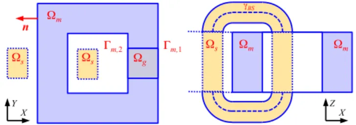
device. The related MMF gathers all the current sources in the slot, for all coils, e.g., coils with different phases in a machine or primary/secondary coils in a transformer. A slot can be generalized to represent the exterior region, including coils as well. Ωm Γm,2 Γm,1 Ωs Ωs n Ωg X Y Ωm Ωs γBS Ωm X Z
Fig. 1. Example of a magnetic region Ωm, including an air gap Ωg, first
con-sidered without leakage flux, via perfect magnetic walls BCs on Γm,1 and Γm,2
in channel slots (XY-plane, left) coupled to end windings coil γBS via BS-SF
model (XZ-plane, right).
B. BS-SF model
With the SPM, the BS SF evaluations can be limited to the material regions Ωm via local VSs [3], [4], instead of the
whole domain with the common method [1]. Such a support reduction already allows to lighten the BS calculations. Then, for accurate combinations with the reaction fields, the BS SFs gain at being projected onto similar function spaces (edge FEs for both source and reaction fields). Also, instead of volume
projections of the SFs in the mesh of Ωm, the SFs gain at being
calculated there via an FE problem with their boundary values as BCs on ∂Ωm, thus already limiting the BS evaluations to
surfaces.
To go one step further, such a preliminary FE problem can be avoided through its inclusion in the main SP p ≡ BS-SF. The key is to think of two successive SPs pa and pb actually solved together (Fig. 2). SP pa first prevents the field to enter Ωm, thus with a reaction field in Ωm opposing the BS field
(di-rect solution of SP q), keeping unchanged the field out of Ωm.
This constraint is simply expressed via both tangential and normal field trace discontinuities of magnetic field hpa and magnetic flux density bpa through Γm, i.e., with ICs with SSs
[n×hpa]Γm=–n×hq|Γm , [n⋅bpa]Γm=–n⋅bq|Γm . (2a-b)
In terms of ap, IC (2b) leads to
[n×apa]Γm=–n×aq|Γm . (3)
The result is an exact zero field in Ωm, with no need of volume
calculation. Then, SP pb considers the actual physical proper-ties in Ωm, with no more VSs, which is a great advantage.
Combining SPs pa and pb thus gives a single SP p that consid-ers the physical properties of Ωm and with the trace
disconti-nuities of SP pa (2a-b) still being valid for its solutions hp and
bp (because SP pb introduces no discontinuities).
BS SF evaluations are thus only required on Γm, which is a
significant advantage. At the discrete level, the IC-SSs in (2a-b)-(3) can be obtained from a mesh projection of only the a BS SF in a layer of FEs along the boundary of Ωm. Details
will be given in the extended paper. An example of result is given in Fig 4. SP p µp=µq σp=σq SP q SP pa + SP pb IN OUT hpa= – hq bpa= – bq hpa = 0 bpa = 0 Ωm Γm IN OUT Ωm µp , σp n hq bq hq bq Ω Ωq Ω hq+hpa= 0 bq+bpa= 0 ! No VS No change outside Biot-Savart Source field µq , σq Inner zero solution Ωm
Fig. 2. BS SF (SP q) for a material region Ωm (SP p): SP p is split into SPs pa
and pb, simultaneously solved, SP pa removing the volume BS solution q in-side Ωm and SP pb considering the actual properties of Ωm, with no need of
VSs for change of properties, but with IC-SSs for the unified SP p.
C. Coupling between MMF and BS-SF models
In 3-D, the slots are generally of two types: 1) a channel surrounded by magnetic regions and possible air gaps (usually considered in 2-D models), coupled through interfaces to 2) an open exterior region for the end windings (3-D effects). It is here proposed to define the channel slots via the MMF model and the end winding regions via the actual consideration of the winding, e.g., via a BS model (Fig. 1, right). With such a cou-pling between MMF and BS-SF models, the flux wall surface has to be extended to these interfaces. Practical details will be given in the extended paper.
D. Volume FE models of conductors
Additional SPs for volume FE models of the source conduc-tors can follow (Fig. 5) [3], [4], for accurate determination of their characteristics (impedances, losses, forces).
The proposed methodology has first been validated on 2-D test problems. It offers tools that allow to reduce the computa-tional effort of the classical approach. When applied up to 3-D problems, its advantages will be shown to be numerous and significant, with quantification of the benefits.
X Y Z
(a) total solution
X Y Z
(b) total sol., in-slot zoom
X Y Z
(c) MMF model sol. Fig. 3. Current source in a slot with air gap (portion of a device): field lines with (a)-(b) classical full model and (c) MMF model.
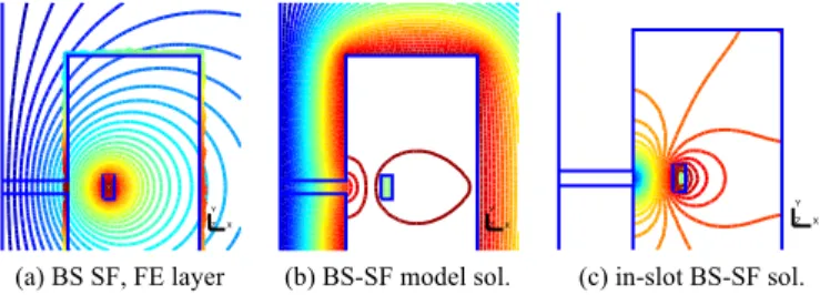
X Y Z (a) BS SF, FE layer X Y Z (b) BS-SF model sol. X Y Z (c) in-slot BS-SF sol. Fig. 4. Current source in a slot with air gap: field lines with BS-SF model; the BS SF is only needed in an FE layer along core boundary Γm; field
discontinu-ities appear (b) through Γm because the total field is obtained in Ωm whereas
the reaction field is obtained outside; due to the simplified shape of the coil, the field distribution in the slot (c) is far from the actual one (Fig. 3b).
X Y Z
(a) volume correction
Z Y X
(b) elevation of volume correction Fig. 5. (a) Field lines of volume correction of coil and its surrounding from BS-SF solution, (b) with its elevation (z-component of a) pointing out the field trace discontinuities; the field distribution (a) is now correct: the total field in the actual coil (same as in Fig. 3b) and the reaction field elsewhere.
ACKNOWLEDGMENT
This work is supported by the F.R.S.-FNRS and the CNPq (project 400452/2014-6).
REFERENCES
[1] P. Ferrouillat, C. Guérin, G. Meunier, B. Ramdane, P. Labie, D. Dupuy, “Computation of Source for Non-Meshed Coils with A–V Formulation Using Edge Elements,” IEEE Trans. Magn., vol. 51, 2015, to appear. [2] P. Dular, R. V. Sabariego, M. V. Ferreira da Luz, P. Kuo-Peng,
L. Krähenbühl, “Perturbation finite element method for magnetic model refinement of air gaps and leakage fluxes,” IEEE Trans. Magn., vol. 45, no. 3, pp. 1400–1403, 2009.
[3] P. Dular, L. Krähenbühl, R.V. Sabariego, M. V. Ferreira da Luz, P. Kuo-Peng and C. Geuzaine. “A finite element subproblem method for posi-tion change conductor systems”, IEEE Trans. Magn., vol. 48, no. 2, pp. 403-406, 2012.
[4] P. Dular, V. Péron, R. Perrussel, L. Krähenbühl, C. Geuzaine. “Perfect conductor and impedance boundary condition corrections via a finite el-ement subproblem method,” IEEE Trans. Magn., vol. 50, no. 2, paper 7000504, 4 pp., 2014.