Case History
Electrical resistivity tomography and distributed temperature
sensing monitoring to assess the efficiency of horizontal
recirculation drains on retrofit bioreactor landfills
Gaël Dumont
1, Tanguy Robert
2, and Frédéric Nguyen
1ABSTRACT
In bioreactor landfills, the recirculation of water can acceler-ate biodegradation and increase gas production. The dedicacceler-ated infrastructure aims at increasing wastewater content over a wide area, with a long-lasting effect. To assess the efficiency of hori-zontal drains in bioreactor landfills, we use electrical resistivity tomography (ERT) and distributed temperature sensing (DTS) to monitor two injection experiments. The first monitoring ex-periment focuses on image resolution and takes advantage of a pseudo 3D ERT data set. This technique successfully high-lights the waste horizontal anisotropy and the crucial role of existing gas wells, acting as vertical preferential flow paths.
The observations are supported by borehole temperature log-ging. The second monitoring experiment focuses on temporal resolution and requires repeated 2D ERT measurements. The hourly acquisition frequency offers better insight on the water-flow dynamics, such as the flow direction and velocity and the water retention trough time. Temperature logging along the horizontal drain indicates that the injected water is distrib-uted over the entire drain length. Altogether, the two recircula-tion experiments inform us on the suitability of large horizontal drains for water recirculation on bioreactor landfills. In conclu-sion, the two geophysical tools provide essential information to determine the most appropriate water-injection protocol in terms of frequency, volume, and flow rate.
INTRODUCTION
The interest in managing landfills as bioreactors in waste man-agement has increased in the past few decades (e.g.,Pohland, 1995;
Reinhart et al., 2002;Kumar et al., 2011). This waste management technology offers several advantages over the conventional sanitary landfill, such as quicker and more complete biodegradation, re-duced long-term pollution risks (and related postexploitation mon-itoring costs), and 15%−30% gain in landfill storage capacity. The landfill gas-production rate is increased during the first years of ex-ploitation, increasing the efficiency of the energy recovery (Kumar et al., 2011). The most limiting factor for the waste biodegradation process is water content. Many efforts have been made to under-stand its effects and to regulate the water content in such complex
and heterogeneous systems (Reinhart and Al-Yousfi, 1996;Šan and
Onay, 2001;Benbelkacem et al., 2010). Bioreactor landfills are de-signed and equipped to enable the monitoring and regulation of the water (and sometimes oxygen) content in the waste mass (e.g.,
Reinhart and Townsend, 1997). The leachate, which accumulates in the lower part of the landfill, is drained, pumped, and reinjected into the upper part. The additional infrastructures required for leach-ate recirculation, such as buried infiltration galleries or horizontal draining layers, have to be included in the bioreactor landfill con-ception (as-built bioreactor). Sometimes, existing traditional land-fills are later turned into bioreactor landland-fills (retrofit). In this context, superficial infrastructures for water addition are often pre-ferred to deep systems because they reduce the risks (odors, explo-sion, etc.) and cost of drilling and deep excavation. The installation
Manuscript received by the Editor 29 November 2016; revised manuscript received 16 August 2017; published ahead of production 02 November 2017; published online 22 December 2017.
1University of Liege, Urban and Environmental Engineering (Applied Geophysics), Liège, Belgium. E-mail: gdumont@uliege.be; f.nguyen@uliege.be. 2University of Liege, Urban and Environmental Engineering (Hydrogeology and Environmental Geology), Liège, Belgium. E-mail: tanguy.robert@uliege.be.
© 2018 Society of Exploration Geophysicists. All rights reserved. B13
of shallow horizontal drains for the injection, sometimes combined with vertical wells, is a common solution (e.g.,Reinhart and Town-send, 1997). Surface infiltration ponds or irrigation systems may also be used. Whatever the type of bioreactor (as-built or retrofit), the quantity of water and the injection fluxes need to be optimized for the system to be efficient in terms of biogas production and leachate or water recirculation. The liquid recirculation should not induce any strong increase in water pressure that would impact the waste-mass stability. The recirculation process must also be de-signed to not exceed the bottom drainage capacity of the landfill (Reinhart and Townsend, 1997).
Measuring the electrical resistivity of waste is an emerging strat-egy for landfill water-content characterization (Grellier et al., 2007;
Imhoff et al., 2007;Moreau et al., 2010;Dumont et al., 2016). The electrical resistivity varies with the water content, composition, tem-perature, and the compression state of the waste (Moreau et al., 2010). For short-term experiments involving recirculation, the water content and temperature changes are the most important effects. The effect of the water contentθ and water electrical resistivity ρwon the porous media bulk resistivityρbis described byArchie’s (1942)law (Wyllie and Gregory, 1953). The latter also involves the sample porosity, saturation, and parameters related to the sample solid ma-trix. Given the difficulty of measuring saturation and porosity on municipal solid waste (MSW) samples, a simplification of Archie’s law is proposed byGrellier et al. (2007), in which only the volu-metric water content is considered (θ ¼ saturation × porosity)
ρb¼ ρwaθ−m; (1)
where a is the tortuosity constant and m is an empiric exponent (a mix of the cementation factor and saturation exponent). Waste with a lower moisture content has higher electrical resistivity.
Campbell et al.’s. (1948)law describes the effect of temperature on electrical conductivity. In most cases, a linear increase (approx-imately 2%) of electrical conductivity is measured for every degree of temperature increase. The validity of this law was checked for MSW samples byDumont et al. (2016)andGrellier et al. (2006b):
σ ¼ σTrefð1 þ cðT − TrefÞÞ; where c ≃ 0.02∕°C
when Tref¼ 25°C: (2)
Noninvasive geophysical methods, such as electrical resistivity tomography (ERT), have been used successfully in the past decade to monitor various physical processes: heat storage and transport (e.g.,Hermans et al., 2014) and saline transport (e.g.,Robert et al., 2012), which are both physical processes occurring in landfills.
In the context of bioreactor landfills, water recirculation induces water content, salinity, and temperature changes in the waste material. Therefore, the interest in noninvasive geophysical meth-ods to estimate the water content and change of water content has grown in the past few years. ERT provides a large spatial coverage of the electrical resistivity of the waste material at depth and can be used to directly derive the water content of the waste (Grellier et al., 2007;Dumont et al., 2016) or to monitor changes linked to water-content variation during recirculation (Morris et al., 2003;Guérin et al., 2004;Grellier et al., 2006a,2008;Clément et al., 2010,2011;
Audebert et al., 2014,2016a,2016b).
In this paper, we first describe the landfill site and technical infra-structure involved in the water-recirculation process (drains, wells,
etc.). Then, we briefly introduce the ERT and distributed temper-ature sensing (DTS) methods. Numerical simulations are used to define a relevant change of resistivity threshold for the water-plume delimitation in the inverted resistivity distribution images of the sec-ond case study.
We used ERT monitoring and the DTS methods to assess large horizontal recirculation drain efficiency for superficial waste humidification in a large retrofit engineered landfill. Two case stud-ies are presented. The first experiment was monitored with a pseudo 3D data set and provided a detailed resistivity distribution around the injection point with a monthly temporal frequency. The second experiment was monitored with a set of four 2D ERT lines that of-fered a less detailed electrical resistivity distribution, but an hourly acquisition frequency to capture the water-flow dynamics.
In both cases, we discuss the results and draw conclusions related to the injected plume extent, the flow anisotropy, the existence of preferential flow paths, and the persistence of the moisture increase because all these elements influence the humidification of the waste and the subsequent biodegradation.
LANDFILL SITE DESCRIPTION
The recirculation experiments were conducted on a large MSW deposit area in Mont-Saint-Guibert, Belgium (Figure1). Here, ap-proximately 11 million tons of waste, mostly composed of MSW, were disposed in a former sand quarry. The site is now 26 ha wide and up to 60 m deep (5.3 million m³), and it presents a dome-shaped topographic profile. The ridge rises to more than 160 m and the border of the site to 135 m. Waste compaction, by use of landfill compactors, likely results in anisotropic, preferentially horizontal, water flow in the waste material. The landfill infrastructure is com-posed of a bottom leachate collection system and a peripheral runoff water-collection system. The landfill gas collection system includes 200 vertical (6.8 wells∕ha) gas extraction wells. These are sealed over the first 3−5 m and surrounded by draining material at a larger depth (Figure1f). Most of these extend from the bottom leachate collection system to the surface. Landfill gas has been valorized for the past 25 years, with more than 1 billion m³ produced. To maintain the gas-production rate for a longer period (and to speed up site mineralization), recirculation drains were installed at two locations on the site.
We estimated the waste material features (water content, temper-ature, and leachate conductivity) from various data acquired on the site (borehole logging and waste and leachate sampling; partially published by Dumont et al., 2016). The waste material in the unsaturated zone is characterized by 25% water content, and the 1 m thick inert cover layer is characterized by 30% water content. Based on borehole measurement data (temperature from K7 and pore-fluid conductivity from K6; see Figure 1a), the temperature and the pore-fluid conductivity increase linearly with depth, from 25°C and7000 μS∕cm at the surface to 42°C and 34;000 μS∕cm at 12 m depth, where the saturated zone starts. Below this, the temper-ature and conductivity are constant with depth. We also calibrated Archie’s law and Campbell’s law for the site (a ¼ 1.53, m ¼ 2.1, and c ¼ 0.022∕°C at 20°C in equations1and2). These values are used for the numerical simulations in the“Resistivity change thresh-old definition” section and for water content rough estimation from electrical resistivity data in the“Results for the first and second ex-periment” sections.
The first experimental site (including the first drain and the first monitoring setup; Figure1aand1d) was located on the ridge, and it is characterized by an average slope of 2.5%, increasing toward the west (up to 6%). At this location, the total thickness of the waste is greater than 50 m. However, the target of the present study is the 15 m thick unsaturated zone. The investigation zone comprises three gas wells (shown in Figure8) as well as a new piezometer (K1) installed in 2012, screened at less than 8 m depth and used for leachate sampling and temperature monitoring.
The second experimental site (including the second drain and the second monitoring setup; Figure 1a and 1e) was located in the western zone of the landfill, parallel to the landfill border. The de-posit site is approximately 30 m thick, and the depth to water table is approximately 12 m. The slope at this location is steeper (14%) toward the northwest. A minimum distance of 5 m was imposed between the drain and gas wells to avoid
prefer-ential vertical flow paths, as we describe in the “Result for the first experiment” section.
MATERIALS AND METHODS Electrical resistivity tomography
The fundamentals of the ERT method have been described by several authors (e.g., Loke et al., 2013;Singha et al., 2015). Briefly, two stainless steel electrodes are used to inject a di-rect electrical current (I, in amperes) into the soil, while two other electrodes are used to measure the resulting potential difference (ΔV, in volts). With modern resistivity meters, hundreds or thousands of data points are collected with differ-ent electrode geometries. We used the multichan-nel ABEM Terrameter LS system (12 acquisition channels) and the multiple-gradient protocol (Dahlin and Zhou, 2006) to reduce the total ac-quisition time needed. This acac-quisition protocol is characterized by a high signal-to-noise ratio. Considering the array description fromDahlin and Zhou (2006), the distance between the two potential electrodes (a) varies from one to three times the electrode spacing, up to s potential dif-ference data points (separation factor, or s) are measured between the current electrodes, which are spaced byðs þ 2Þ × a (Figure2). The data set for the first monitoring setup (the pseudo 3D monitoring consists of a set of orthogonal 2D lines, later inverted with a 3D forward model iter-ative process) is composed of 5084 data points,
and the data set for the second monitoring setup (2D monitoring) is composed of 1152 data points.
Each data set was then inverted to produce a 2D or 3D represen-tation of the bulk electrical resistivity distribution that explains the measured data. Through this iterative process, an objective function (equation3, Tikhonov and Arsenin, 1977) is minimized:
Φ ¼ kWdðd − fðmÞÞkpþ λkWmmkp: (3)
The objective function is composed of the data misfit constraint and the regularization constraint (Oldenburg and Li, 1994). The
operator kkp represents the Lp-norm operator, W
d is the data
weighting matrix (based on an estimation of the data uncertainties), f is the forward operator, Wmis the model roughness matrix, andλ
is a regularization parameter.
The data for the first experiment were inverted using the inversion code Res3DInv (Geotomo Software, 2011) with robust data misfit and regularization constraints (L1-norm). The robust regularization constraint, referred to as blocky inversion (Loke et al., 2003), al-lowed us to obtain sharper boundaries in our resistivity images.
The data for the second experiment were inverted using the L1-norm with the CRTomo software (the software description may be found inKemna, 2000). In CRTomo, the data error matrix Wd
con-tains an estimation of the error level on the data, based on reciprocal measurements (LaBrecque et al., 1996). In this study, the envelope of the reciprocal errors (Slater et al., 2000), which provided a
Figure 1. (a) General view of the CETEM site with experimental sites 1 and 2 (see the enlarged views) and the borehole K6 location, (b) location of the site in Belgium, (c) graphical legend for frames (a, d, and e), (d) enlarged view of the first experimental site (with drain 1, the pseudo 3D ERT layout and borehole K1), (e) enlarged view of the second experimental site (with the first section of drain 2, the 2D ERT layout and bore-hole K7), and (f) vertical sections of drains 1 and 2.
Figure 2. The multiple-gradient electrode layout used for all data acquisition and simulation throughout the paper (a is the electrode spacing, and s is the separation coefficient).
conservative error model, was modeled by a relative error of 1% and an absolute error of0.0005 Ω (measured electrical potential divided by the injected electrical current). The inversion process stops when the field data set is fitted within this error level (i.e., the error weighted χ2 of the data misfit reaches one). The regularization parameterλ is optimized at each iteration, and it is increased at the final iteration to exactly fit the assumed level of noise (Kemna, 2000).
Changes of electrical resistivity distribution through time were studied with independent time-lapse inversions using the same soft-ware as previously mentioned. For that purpose, the ERT data were acquired at the same place at different times with the same acquis-ition protocol. The electrodes were left in place for the entire mon-itoring duration. This procedure allowed the monmon-itoring of dynamic processes such as changes in water content, salinity, or temperature. The time step needed depends on the observed phenomenon. It is often limited by the acquisition time of a single resistivity data set.
Resistivity change threshold definition
In this study, we were mainly interested in determining the in-jected liquid plume extent, flow anisotropy and preferential flow paths, and persistence of the moisture increase. This can be achieved by observing the relative water-content changes, as pro-posed byClément et al. (2010). To select a suitable threshold to delimitate the water plume extent for the second experiment, we used a synthetic model representing our second field site. The def-inition of the threshold depends on many factors starting with the inversion algorithm and parameters (regularized inversion induces a smoothed electrical resistivity distribution), the magnitude of the changes (initial water content, added water content), the water
dis-tribution inside the water plume (homogeneous or not), or the size and depth of the water plume. It can also be affected by the propa-gation of data noise in the inversion (Hermans et al., 2012;Robert et al., 2012). The background condition is a horizontally layered model (77.5 m wide by 28 m deep; the section is cropped in Figure 3a) representing our test site. It is composed of waste material with 25% water content, overlaid by a 1 m thick inert cover layer with 30% water content. Temperature and leachate conduc-tivity data, used to simulated potential difference data, are based on borehole data from K6 and K7, as described in the“Landfill site description” section. A 20 m wide and 5 m thick water plume is added in the center of the section with various water-content changes, depth, water-content distribution changes inside the plume, and various initial water content in the waste material (Figure3a).
Water-content changes were converted into resistivity changes using equations1and2. Using the CRTomo finite-element code, ERT data were simulated (finite-element method) with a regular grid with 0.25 × 0.125 m elements. For this purpose, we use the same electrode layout and spacing for the numerical simulation and the second field data acquisition (multigradient protocol with 2.5 m spacing, with a total of 1152 data points). Then, Gaussian noise (identical to the noise measured on the experimental site with reciprocal measurements) was added to simulated potential data. The latter are inverted with a regular grid with1.25 × 0.5 m ele-ments (identical to the grid used for the field case). The change of resistivity between the resistivity distribution with and without the added water plume was compared with the inverted resistivity distributions. The vertical profiles at the center of the plume for the various considered cases are presented in Figure3b–3e.
The reference simulation, a5 × 20 m plume at 6 m depth, consisting of a 5% (absolute) water content increase (from 25% to 30% water con-tent, corresponding to a 20% relative change of water content and a−31.5% relative change of resistivity), is common for Figure 3b–3e
(red curves). The effect of the added water content (3%, 5%, and 8% absolute water content increase) is presented in Figure3b. The magni-tude of the change was correctly estimated, but the inverted resistivity change distribution was smoothed over a wide thickness. Therefore, the choice of a resistivity change threshold was needed for the delimitation of the water plume. A threshold equal to 70% of the observed maximum magnitude fairly delimits the water plume, whatever the simulated water-content changes.
The effect of the water-plume depth is pre-sented in Figure3c. The same resistivity thresh-old definition (70% of the maximum resistivity change) can be used for the 4 and 6 m deep plumes. For the 8 m deep plume, the inverted resistivity distribution is smoothed over a large area due to the loss of resolution and sen-sitivity with depth of ERT images (e.g.,Hermans et al., 2016a). The maximum resistivity change magnitude was underestimated (25% instead of 31.5%). The thickness of the plume is Figure 3. (a) Schematic 2D material section, modeled water plume, and ERT acquisition
protocol used for data simulation. Change of resistivity response for various water-plume features (model, continuous lines; inverted distribution, dashed lines; and thresh-old used for plume delimitation, vertical dotted lines); (b) resistivity change response to added water content (þ3%, 5%, and 8% water content increase in green, red, and blue, respectively); (c) resistivity change response to plume depth (4, 6, and 8 m plume depth in blue, red, and green, respectively); (d) resistivity change response to added water-content distribution (homogeneous, more at the top, more in the center, and more at the bottom water distribution in red, green, yellow, and blue); and (e) resistivity change response to the initial water content (20%, 25%, and 30% initial water content in blue, red, and green, respectively).
overestimated when using the previously described threshold for interpretation.
The influence of the added water-content distribution in the water plume is presented in Figure3d. Although the total added water content for the whole water plume is constant, most added water content is located close to the surface, at the center of the plume, or at the bottom part of the water plume (respectively, the green, yellow, and blue lines in Figure3d). The same resistivity threshold definition (70% of the maximum resistivity change) can be used for the two first cases. The thickness of the plume was overestimated for the third scenario.
The influence of the initial water content (20%, 25%, and 30% for blue, red, and green curves, respectively), for a constant relative change in water content (þ20%), is presented in Figure3e. Al-though the relative electrical resistivity changes are identical in the model, the responses are slightly different for the three cases. However, the resistivity change threshold previously defined can still be used.
From these numerical simulations, we concluded that a threshold of 70% of the maximum change magnitude can be used as a first approximation for shallow water plume delimitation. However, for water content changes at greater depth, the change in magnitude is underestimated and the plume thickness is overestimated. Alterna-tive regularization operators (“variogram based” or “minimum gra-dient support”) can be used to try to reduce smoothing (Hermans et al., 2016a;Nguyen et al., 2016).Audebert et al. (2014)propose to use multiple inversions (while varying the inversion parameters) to delineate the plume extent. Recently,Hermans et al. (2016b)
propose a prediction-focus approach to directly derive property changes from ERT data, avoiding inversion and regularization. However, their methodology has only been tested on synthetic cases.
Temperature monitoring
We used DTS for temperature monitoring with an AP-sensing “linear pro series.” The method is based on Raman optical time-do-main reflectometry (Dakin et al., 1985;Hurtig et al., 1994). A laser pulse is emitted into an optical fiber. At every location on the fiber, part of the energy is backscattered to the source. The traveltime de-termines the exact position along the fiber of the observation point, and the light-frequency spectrum is temperature dependent. The temperature along the fiber is determined by the relative intensity of Raman Stokes and anti-Stokes signals. The minimum spatial res-olution is 50 cm, the minimum temperature resres-olution is 0.1°C, and the minimum temporal resolution is 30 s. However, these values are interdependent. This temperature sensing system was experimen-tally calibrated in the laboratory by use of cold and hot reference temperature baths. Because we were more interested in temperature changes than in absolute temperature values, calibration was not performed on the field.
Descriptions of the experiments
The first recirculation drain was composed of a 110 mm (diam-eter) perforated tube dug to a 2 m depth and surrounded by a 3 × 1 m drainage material section (gravel from the nearby sand quarry, extending from 1 to 4 m in depth). The injection point was the western and lowest part of the drain (Figure1). The first re-circulation experiment started in March 2013 and lasted for one year.
The first experiment was monitored with a pseudo 3D data set and provided a detailed resistivity distribution around the injection point with a monthly temporal frequency. The monitoring area covered a50 × 50 m site centered on the starting point of the drain. The electrode layout for the ERT monitoring covered a 1 ha area. The pseudo 3D acquisition sequence was composed of 20 profiles of 16 electrodes (northeast–southwest) and 12 profiles of 24 electro-des (northwest–southeast). The data set is composed of 5084 data points. The electrode spacing (2.5 m in northwest–southeast direc-tion and 5 m in the northeast–southwest direcdirec-tion) offered a com-promise (assessed by preliminary numerical simulations) between the spatial resolution and the depth of investigation. For each profile, four electrodes (the first two and the last two) were located 10 and 20 m away from the test zone to increase the depth of in-vestigation in the central zone. The electrode contact resistance was generally low (approximately 100 Ω), but some very high values (greater than10;000 Ω, due to dry sand impeding a good electrical contact between the electrode and the cable connector) induced data loss or repeatability errors. Data with repeatability errors greater than 5% (1%–5% of the full data set) were discarded. All inversions converged with root-mean-square (rms) error values between 4% and 8%.
The pseudo 3D data set acquisition lasted for two working days (the ERT cables were not left on the site due to heavy plant traffic, but the electrodes were) and were acquired monthly. The back-ground acquisition (contaminated by a previous test of the pump) was conducted in March 2013, two weeks before the recirculation experiment started (Figure4). Acquisition periods with no precipi-tation and no liquid recirculation were favored (at least two days before and during the acquisition) for the monthly pseudo 3D data set acquisition. The injection sequence, presented in Figure4and Table1, was managed by the landfill owner and did not follow a repetitive pattern. Weeks preceding the acquisitions were character-ized by various injected volumes. As an example, a small quantity (0−1000 m3) of water was recirculated during the period preceding
the acquisition of data sets 1, 3, and 5. In contrast,2000−3000 m3 were recirculated prior to the acquisition of data sets 2, 4, and 6. The second data set, acquired in June 2013, followed the longest injec-tion period (Figure4). Vertical temperature profiles were measured with a DTS system in a well (K1) specifically drilled and equipped for this experiment to detect the water-plume arrival during the first
Figure 4. Injection sequence for the first recirculation experiment (daily injected volume: red columns; cumulated volume: blue line), and acquisition days for the pseudo 3D ERT data sets.
injection phase (Table1). To capture temperature changes in the unsaturated zones, the fiber optic was in contact with the borehole tubing. Temperature profiles were also acquired monthly during the one-year monitoring experiment.
For the second experiment, the injection drain was composed of four sections of 50 m, separated by 10 m wide clay filling (Figure1). The drain was composed of a 110 mm perforated tube, surrounded by draining material (Table1). A second perforated pipe, installed parallel to the recirculation drain, was equipped with a fiber optic for temperature monitoring (Figure 1f). Different recirculation experiments were conducted in the different drain sections. Two injection tests (60 and275 m3) conducted in drain 2 (section 1) are presented in this study. The electrode layout for the ERT monitoring was composed of 128 electrodes for every 50 m drain section (Figure1). Two 32 electrode (77.5 m long, 2.5 m spacing) profiles were par-allel to the drain (2.5 and 15 m downslope), and two 32 electrode profiles were perpendicular to the drain (12.5 m apart). Each profile acquisition lasted for 13 min. The acquisition of the four 2D profiles allowed an hourly monitoring frequency, more adequate for the recirculation dynamics monitoring than the pseudo 3D acquisition. The full data set was composed of 1152 data points and was acquired in this specific order: profile southwest, northeast, southeast, and then north-west. Due to the permanent site installation, the electrode contact resistance was generally a few hundred ohm, and it was always lower than 1000Ω. The total monitoring period lasted for 15 months. The temperature was measured along the injection drain to spatially control the injec-tion process.
RESULTS FOR THE FIRST EXPERIMENT Background electrical resistivity distribution
The injection pump was tested for several days (the injected volume is estimated to several thou-sand cubic meter) prior to any ERT monitoring acquisition, the background electrical resistivity distribution is influenced by this recirculated liquid, which displays low resistivity values (Figure 5). The initial resistivity distribution is not homogeneous. The drain location is charac-terized by higher electrical resistivity as the drainage material rapidly desaturates. The leach-ate plume is characterized by very low resistivity (<4 Ωm), characteristic of saturated waste (4 Ωm for a highly saturated perched water table and1 Ωm for the saturated zone at depth; Du-mont et al., 2016). It extends from 2 to 6 m depth, starting from the drain and flowing 15 m away from the drain toward the west. A total volume of30 × 30 × 4 m was impacted by the pump test. Resistivity drops from 10 to15 Ωm outside the plume, to2−4 Ωm inside the plume. Given the temperature and leachate conductivity estima-tions presented in the“Materials and methods” Table 1. Summary of recirculation experiments 1 and 2: drain geometries,
injection timing, temperature monitoring system, and ERT monitoring features.
Site 1 Site 2 (drain section 1)
Drain features 110 mm perforated tube, 2 m depth
110 mm perforated tube, 4 m depth
400 m long 50 m long
100−120 m3∕h injection 100−120 m3∕h injection
Injection timing Pump test: approximately
1000 m3 Pump test:120 m 3
(19–27/2/2013) (late 6/2014) 11;000 m3injected in one year
18/3/13–18/3/2014 Individual injection experiment:60 (30/7/2014) and275 m3 (11/8/2014)
T° data Vertical profile in borehole K1 Along injection drain
ERT monitoring 12 lines of 24 electrodes (2.5 m spacing)
Four lines of 32 electrodes (2.5 m spacing) 20 lines of 16 electrodes (5 m spacing) 1152 data points Hourly (30/7/2014–19/8/2014) 5084 data points Monthly (5/3/2013, 24/4/2013, 31/5/2013, 4/7/2013, 27/8/2013, 23/9/2013, 18/11/2013, 12/2/2014, 18/3/2014)
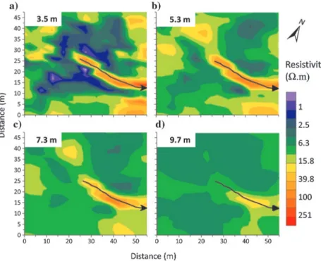
Figure 5. First recirculation experiment: background electrical resistivity distribution (influenced by a preliminary test of the pump). The electrical resistivity distribution is presented for several depth slices: (a) 3.5, (b) 5.3, (c) 7.3, and (d) 9.7 m. The black curve indicates the injection drain location; rms error = 5.3%.
section (30°C and15;600 μS∕cm at 5 m depth), this resistivity drop corresponds to an increase of water content from 25%–30% (dry waste) to 45%–65% (saturated waste). The additional water content resulting from the pump test is500−1500 m3, which is smaller than the estimated injected volume during the pump testing (7 h a day for seven days, the pump maximum flow rate being approximately 100 m3∕h). A proportion of the water injected during the injection
test is thought to have escaped from the monitored area.
2D temperature monitoring during the first injection event
The first monitored injection occurred in March 2013. Because the injected fluid is colder than the waste material, a temperature decrease is noticed between the 2 and 6 m depth at the borehole K1 location (Figure6), confirming a mainly horizontal water flow in the waste material. Because borehole K1 is located close to the drain position, the temperature drops from 30°C to 20°C as a result of cold fluid injection. However, the temperature decrease in the entire test zone was not investigated.
Pseudo 3D ERT monitoring of the one-year recirculation experiment
For the long-term variation of electrical resistivity, a pseudo 3D data set was acquired every month. The temperature vertical profile was measured in borehole K1 (Figure7a). The average air-temper-ature data were provided by the Chastre meteorological station (5 km from the site) (Figure7a).
The electrical resistivity changes between the background acquis-ition and the following months are presented in Figure7b. Inverted resistivity data at 3.5 m depth are averaged over a35 × 30 m area for the“inside plume” values and a 5 m wide perimeter around the plume for the“outside plume” values. Outside the leachate plume influence (Figure7b), the resistivity slightly changes in accordance with the outside temperature. Inside the waste plume volume (Fig-ure7b), two antagonist effects take place. The injected fluid (leach-ate mixed with fresh w(leach-ater) is less conductive and colder than the waste material. Given that the waste material is initially highly sa-turated, a new arrival of colder and diluted leachate induces a pore-fluid resistivity increase, without effectively increasing the water content. This was observed after the longest injection period for data sets 2, 4, and 6 (Figure7b). After one year of monitoring, data set 8 (March 2014) is characterized by a similar electrical resistivity distribution to the background data set (March 2013).
Between March 2012 and March 2013, more than10;000 m3of water was recirculated through the injection drain. However, from our results, the total leachate plume extension did not significantly vary with time. The amount of additional water contained in this plume is estimated at approximately500−1500 m3, and it was pro-vided by the pump test. The remaining amount of water apparently reached the saturated zone and then the landfill leachate collection system.
We use data set 2 (June 2013) to illustrate the role of gas wells in the recirculated water flow. The electrical resistivity distribution from 3.5 to 9 m depth is presented in Figure8. At the drain level (3.5 m depth slice), the leachate plume extends horizontally over a 30 × 30 m area and is limited by three gas wells (screened at less than a 5 m depth) located around the monitored area. The new bore-hole (K1) does not influence the leachate flow because it is screened
only at less than a 8 m depth (Figure8a). At a greater depth (5.3 m), the resistivity is higher and the saturation is probably lower. In the northern area, the leachate seems to infiltrate slowly at the greater depth. In the southern area, the vertical infiltration is directly corre-lated to the presence of gas wells (Figure 8b). We make the assumption that these gas wells are affecting the vertical flow be-cause they are surrounded by draining material. These act as vertical preferential flow paths where the leachate“sinks” toward the satu-rated zone of the landfill, as confirmed by the 7.3 and 9 m electrical resistivity depth slices (Figure8cand8d). A small part of this leach-ate is redistributed around the gas well in deeper waste layers, as illustrated by a northwest to southeast vertical resistivity profile in-tersecting with the most eastern gas well of the site (this well is not equipped with a metal casing; Figure8e). However, a large propor-tion of the recirculated liquid directly reaches the saturated zone, as confirmed by leachate analysis from a piezometer located at 70 m southwest of K1 (Figure8), where leachate samples from the satu-rated zone appear very diluted after several months of recirculation.
Figure 6. First recirculation experiment: changes in the vertical temperature distribution, measured in borehole K1, during the first monitored injection event.
Figure 7. First recirculation experiment: one-year monitoring sum-mary. (a) Temperature variation in borehole K1 (3.5 m depth) mea-sured with the DTS and air temperature data from the nearby Chastre meteorological station. (b) Average electrical resistivity at 3.5 m depth inside and outside the area influenced by the injected water. The black crosses indicate DTS and ERT acquisition days.
RESULTS FOR THE SECOND EXPERIMENT
The implementation of the second recirculation drain intended to avoid injection pitfalls encountered in the first experiment (the ac-cumulation of water at the first drain lowest point and preferential flow paths through the gas wells). The second drain was divided
into four horizontal 50 m long sections. Only the ERT results for drain section 1 are presented in the study.
Background electrical resistivity distribution (section 1)
The background resistivity distribution is heterogeneous (Figure 9). The cover layer ap-pears more resistive in the northwest zone, prob-ably due to the higher vegetation density and related root water uptake. The drain location is clearly depicted by a resistive spot on west and east profiles because the drainage material is desaturated. Resistivity decreases with depth as the pore-fluid conductivity and temperature increase, which is the characteristic vertical elec-trical resistivity profile in waste deposits. Given the electrical resistivity distribution, and using the temperature and leachate conductivity distri-butions described in the“Materials and methods” section, the initial water content in the unsatu-rated zone is 27.5% on average (6.5% standard deviation).
Drain temperature monitoring
During every injection phase, the temperature inside the horizontal drain is monitored with a DTS system. This procedure allows us to esti-mate the horizontality of the recirculation drain to detect possible lower points where water would preferentially accumulate and infiltrate (Figure 10). The results are presented for the 60 m3injection for drain section 1. The injection
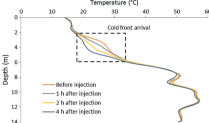
rate is approximately 100−120 m3∕h. The in-jected liquid arrival is always characterized by a temperature decrease. The results for the drain section 1 are illustrated in Figure10. The initial temperature varies between 30°C and 35°C. The peak in tempera-ture at the middle of the drain section corresponds to the location of a gas extraction well with a high yield. During the injection phase, the temperature rapidly decreases over the entire length of the drain, giving indications to the horizontality of the drain and its effec-tiveness.
2D ERT monitoring of liquid recirculation dynamics (section 1)
During the water recirculation experiment in drain section 1, we monitored the electrical resistivity every hour. A total of four 2D ERT profiles were acquired for each time frame. Given the dynam-ics of the observed experiment, a 2D inversion of each individual profile was favored to 3D inversion of the full data set. The southern tomography, along the drain, certified that the drain was used on its entire length. The other profiles were used to assess the recirculated liquid flow behavior and the added moisture residence time as a function of the injected volume.
The 60 m³ injection test was monitored for one week. Data are presented for several time periods after the injection time: 1, 2, 3, 12, 18, and 48 h (Figure11). To ease the visualization, values lower Figure 8. First recirculation experiment: electrical resistivity distribution after a large
injection period (ERT data set number 2; see Figure4). The electrical resistivity dis-tribution is presented for several depth slices: (a) 3.5, (b) 5.3, (c) 7.3, and (d) 9.7 m. The black curve indicates the injection drain location, the red line indicates the vertical ERT section location, the black dots indicate gas wells, and the red dot in-dicates the piezometer K1. (e) Vertical transect intersecting the most eastern gas well of the site; rms error = 8.1%.
Figure 9. Second recirculation experiment: background electrical resistivity distribution around the first section of the second drain. Profiles are named according to the intermediate cardinal directions, coordinates are“Belgian Lambert 1972”; χ2¼ 1.
than 10% are depicted as blank in Figures11and12. This corre-sponds to a water-content change less than 2%. Resistivity changes below this limit are likely related to the smoothing effect inherent to the ERT data inversion, or to noise. The black line indicates the “70% of local maximum” threshold defined in the material and methods section. The southeast profile, located along the drain, shows that the injection drain is used over almost its entire length, except from the most southwestern area (the 45 m large plume, whereas the drain is 50 m long). Then, the leachate plume extension changes during the first 3 h following the injection. It at first has a smaller horizontal extent (Figure11a). Then, the horizontal extent increases along the field slope, while the thickness and the maxi-mum change value decreases. For the first time frame, the plume extent is approximately2000 m3when using the 70% threshold de-scribed in the “Materials and methods” section. The observed changes are extremely high (<−40%) and are focused on the in-jection drain (Figure11a). This is partially accounted for by the initially poorly saturated media surrounding the drain (resistivity change from 25 to15 Ωm). The leachate plume extent is approx-imately2000 m3, which corresponds to an average water-content increase of 3% (volumetric water content; 60∕2000 m3). Then, as the injected liquid flows from the drain toward the northwest di-rection, the resistivity change magnitude decreases (−25%, from 24 to 18 Ωm) close to the drain location and increases down-slope (Figure 11c). The leachate plume extent is now approximately 2500 m3, which corresponds to an average water-content increase
of 2.4% (60∕2500 m3). Three hours after the injection, water
ar-rives at the bottom part of the test field, close to the peripheral drain (Figure11c, profile southwest). This was observed in the field, but it is not visible on the tomography because the resistivity changes re-main less than 10%. The water-flow velocity along the horizontal direction is approximately10 m∕h. During the following two days, the magnitude of the resistivity progressively decreases. After 48 h, only a small fraction of the waste mass has its water content in-creased by a few percent (Figure11f). The water retention time is small, probably due to the high horizontal permeability of the waste material and the slope of the field test.
The275 m3injection experiment occurred 12 days after the first injection test. The injected volume is deliberately large to highlight the anisotropy and the heterogeneity of the ground-water flow.
Because the injection time lasted for 2.5 h, the electrical resistivity data are recorded before, during, and after the injection period. Data ac-quired during the injection (Figure 12a–12c) need to be handled with care because the dynam-ics of the water injection and flow are not neg-ligible in comparison with the acquisition time needed for a full data set. During the first hour of injection (Figure12a), it can be seen that less liquid has been recirculated before the acquisi-tion of the southwest profile than before the ac-quisition of the northeast profile. At the end of the injection period (Figure12c), the southeast profile shows that the drain is saturated along its entire length, even in the most western area. The anisotropic behavior is clearly depicted on the two perpendicular tomographies. The vertical
infiltration is very slow, whereas the horizontal flow is quick and follows the topographic profile of the surface (Figure12d–12f), as a result of the waste material anisotropy. Looking at the water-flow velocity, the water plume front is located 8, 20, 25, and 33 m down the drain in Figure12a–12d, respectively. This represents a horizon-tal average water-flow velocity of8 m∕h when a large volume of water is injected. No vertical flow of the plume was observed using ERT. Two hours after the end of the injection (Figure 12e), the plume volume is approximately 8000 m3 and the water content has been increased by only 3.5% (275∕8000 m3) on average, which
is slightly larger than for the 60 m³ injection experiment. The larger the injected volume, the larger the impacted waste volume, but the water content increases are similar. In the two perpendicular tomog-raphies, the velocity of the injected water and the retention times differ, confirming very heterogeneous flow properties in the waste material. On the southwest profile, the water plume does not extend very fast. When the injection is stopped (Figure12d), the resistivity changes magnitude slowly decreases and the injected water stays in the ground for a few days. This could be accounted for by a rather low permeability and/or a rather high water retention capacity, whose effects can hardly be differentiated with this single experi-ment. In the meantime, on the northeast profile, the water flows toward the border of the landfill and emerges at the surface only
Figure 10. Temperature monitoring along the second injection drain: Temperature data were recorded before the recirculation ex-periment (red line), 2 min after injection started (green line), and 4 min after injection started (blue line).
Figure 11. Second recirculation experiment: ERT monitoring during the injection of 60 m³ of water. The following time frames are presented: (a-f), respectively, 1, 2, 3, 12, 18, and 48 h after the injection. The black line indicates the“70% of local maxi-mum” threshold. The orientation and dimensions are identical to Figure9;χ2¼ 1.
2 h after the injection was stopped (Figure12e). Two days after the recirculation (Figure 12i), no clear evidence of water addition is seen on this tomography. The water recirculation is rather not very efficient at this location and has to be regularly repeated to maintain the water content increase.
CONCLUSION
We used ERT and DTS to assess large horizontal recirculation drain efficiency for superficial waste humidification in a large retrofit engineered landfill. We were particularly interested in the injected liquid plume extent, preferential flow paths, flow aniso-tropy, and persistence of the moisture increase. The first experiment was monitored with a pseudo 3D data set and provides a detailed resistivity distribution around the injection point with a monthly temporal frequency. On the one hand, these results highlight the water flow horizontal anisotropy and the role of gas wells on the vertical transfer of water. On the other hand, the monthly acquisition failed to capture the water-flow dynamics. The measurement of the vertical temperature in K1 detected the water-plume arrival during the injection phase between 2 and 6 m depth, at the same depth as the drain, confirming the horizontal water-flow anisotropy due to waste compaction. The monthly temperature recordings showed a temperature difference of 20°C during the year at shallow depths (3–4 m) that explain electrical resistivity variations outside the re-circulated water-plume influence.
The second experiment was monitored with temperature measurements along the drain and a set of four 2D ERT lines. The temperature hori-zontal profile confirmed that for both injected volumes (60 and 275 m3), the drain sections were used on their entire length. The ERT mon-itoring offered a less detailed electrical resistivity distribution than the pseudo 3D acquisition, but a much higher (hourly) acquisition frequency that successfully captured the water-flow dynam-ics. For our field case, characterized by the heterogeneous initial water-content distribution and water-content changes, the resistivity relative change distributions should be interpreted with care. Based on numerical simulation, we proposed the use of a resistivity change threshold equal to 70% of the local maximum that fairly delimited the water-plume extension. For the 60 and275 m3 injection experiments, the water-plume extension and evolution through time is clearly depicted. This observation offered valuable information on flow anisotropy, heterogeneity, and water-plume persistence over time.
The two recirculation experiments together in-form us on the suitability of a large horizontal drain for water recirculation on a large retrofit landfill. Multiple short drain sections (site 2), for which the horizontality is better controlled, should be favored compared with a single long drain (site 1) to distribute the injected fluid equally over the entire site surface. The waste compaction results in mainly horizontal leachate flow. Therefore, the fluid recirculation mainly impacts superficial unsaturated waste layers. Although the occurrence of short vertical drains may favor water distribution over a larger waste volume, deep vertical gas wells (extending from the bottom leachate collec-tion system to the surface) create direct flow paths between the sur-face and the saturated zone, hampering the unsaturated waste mass humidification because they connect the recirculation drain directly to the leachate drainage system. The water-content persistence through time is extremely variable, from a few hours to a few days on test 2, where the slope is steep, to several weeks on site 1, where the slope is low. These factors need to be considered for future hori-zontal drain implementation and to set up the injection volume and frequency.
ACKNOWLEDGMENTS
This research is part of the MINERVE project (Plan Marshall2. vert, pôle GreenWin). We would like to thank SHANKS, the leader of the research program for technical support and access to the site, the CWBI (Industrial Biochemistry and Microbiology Unit) for leachate sample analysis, and the Royal Observatory of Belgium for logistical support.
REFERENCES
Archie, G. E., 1942, The electrical resistivity log as an aid in determining some reservoir characteristics: Transactions of the American Institute of Mining and Metallurgical Engineers, 146, 54–67, doi:10.2118/942054-G.
Figure 12. Second recirculation experiment: ERT monitoring during the injection of 275 m3of water. The following time frames are presented: (a-c), during the injection,
respectively, 1, 2, and 3 h after the injection started; (d-i), respectively, 1, 2, 3, 12, 24, and 48 h after the injection ended. The black line indicates the 70% of local maximum threshold. The orientation and dimensions are identical to Figure9;χ2¼ 1.
Audebert, M., R. Clément, S. Moreau, C. Duquennoi, S. Loisel, and N. Touze-Foltz, 2016a, Understanding leachate flow in municipal solid waste landfills by combining time-lapse ERT and subsurface flow modelling— Part I: Analysis of infiltration shape on two different waste deposit cells: Waste Management, 55, 165–175, doi:10.1016/j.wasman.2016.04.006. Audebert, M., R. Clément, N. Touze-Foltz, T. Günther, S. Moreau, and C.
Duquennoi, 2014, Time-lapse ERT interpretation methodology for leach-ate injection monitoring based on multiple inversions and a clustering strategy (MICS): Journal of Applied Geophysics, 111, 320–333, doi:
10.1016/j.jappgeo.2014.09.024.
Audebert, M., L. Oxarango, C. Duquennoi, N. Touze-Foltz, N. Forquet, and R. Clément, 2016b, Understanding leachate flow in municipal solid waste landfills by combining time-lapse ERT and subsurface flow modelling— Part II: Constraint methodology of hydrodynamic models: Waste Man-agement, 55, 176–190, doi:10.1016/j.wasman.2016.04.005.
Benbelkacem, H., R. Bayard, A. Abdelhay, Y. Zhang, and R. Gourdon, 2010, Effect of leachate injection modes on municipal solid waste degradation in anaerobic bioreactor: Bioresource Technology, 101, 5206–5212, doi:10
.1016/j.biortech.2010.02.049.
Campbell, R., C. Bower, and L. Richards, 1948, Change of electrical con-ductivity with temperature and the relation of osmotic pressure to elec-trical conductivity and ion concentration in soil extracts: Soil Science Society of America Proceedings, 13, 66–69, doi: 10.2136/sssaj1949
.036159950013000C0010x.
Clément, R., M. Descloitres, T. Günther, L. Oxarango, C. Morra, J.-P. Laurent, and J.-P. Gourc, 2010, Improvement of electrical resistivity tomography for leachate injection monitoring: Waste Management, 30, 452–464, doi:10.1016/j.wasman.2009.10.002.
Clément, R., L. Oxarango, and M. Descloitres, 2011, Contribution of 3-D time-lapse ERT to the study of leachate recirculation in a landfill: Waste Management, 31, 457–467, doi:10.1016/j.wasman.2010.09.005. Dahlin, T., and B. Zhou, 2006, Multiple-gradient array measurements for
multichannel 2D resistivity imaging: Near Surface Geophysics, 4, 113–123. Dakin, J. P., D. J. Pratt, G. W. Bibby, and J. N. Ross, 1985, Distributed op-tical fibre Raman temperature sensor using a semiconductor light source and detector: Electronics Letters, 21, 569–570, doi:10.1049/el:19850402. Dumont, G., T. Pilawski, P. Dzaomuho-Lenieregue, S. Hiligsmann, F. Delv-igne, P. Thonart, T. Robert, F. Nguyen, and T. Hermans, 2016, Gravimet-ric water distribution assessment from geoelectGravimet-rical methods (ERT and EMI) in municipal solid waste landfill: Waste Management, 55, 129– 140, doi:10.1016/j.wasman.2016.02.013.
Geotomo Software, 2011, RES3DINV ver. 2.22, 3D resistivity and I.P. In-version using the least-squares method: Geotomo Software.
Grellier, S., R. Guérin, H. Robain, A. Bobachev, F. Vermeersch, and A. Tab-bagh, 2008, Monitoring of leachate recirculation in a bioreactor landfill by 2-D electrical resistivity imaging: Journal of Environmental and Engineer-ing Geophysics, 13, 351–359, doi:10.2113/JEEG13.4.351.
Grellier, S., K. Reddy, J. Gangathulasi, R. Adib, and A. Peters, 2006a, Elec-trical resistivity tomography imaging of leachate recirculation in Orchard Hills landfill: Presented at the SWANA Conference.
Grellier, S., K. Reddy, J. Gangathulasi, R. Adib, and C. Peters, 2007, Cor-relation between electrical resistivity and moisture content of municipal solid waste in bioreactor landfill: Geotechnical Special Publication, 163, 1–14.
Grellier, S., H. Robain, G. Bellier, and N. Skhiri, 2006b, Influence of tem-perature on the electrical conductivity of leachate from municipal solid waste: Journal of Hazardous Materials, 137, 612–617, doi:10.1016/j.
jhazmat.2006.02.049.
Guérin, R., M. L. Munoz, C. Aran, C. Laperrelle, M. Hidra, E. Drouart, and S. Grellier, 2004, Leachate recirculation: Moisture content assessment by means of a geophysical technique: Waste Management, 24, 785–794, doi:
10.1016/j.wasman.2004.03.010.
Hermans, T., A. Kemna, and F. Nguyen, 2016a, Covariance-constrained dif-ference inversion of time-lapse electrical resistivity tomography data: Geophysics, 81, no. 3, E311–E322, doi:10.1190/geo2015-0491.1. Hermans, T., F. Nguyen, T. Robert, and A. Revil, 2014, Geophysical
meth-ods for monitoring temperature changes in shallow low enthalpy geother-mal systems: Energies, 7, 5083–5118, doi:10.3390/en7085083. Hermans, T., E. Oware, and J. Caers, 2016b, Direct prediction of spatially
and temporally varying physical properties from time-lapse electrical re-sistance data: Water Resources Research, 52, 7262–7283, doi:10.1002/
2016WR019126.
Hermans, T., A. Vandenbohede, L. Lebbe, and F. Nguyen, 2012, A shallow geothermal experiment in a sandy aquifer monitored using electric resis-tivity tomography: Geophysics, 77, no. 1, B11–B21, doi: 10.1190/
geo2011-0199.1.
Hurtig, E., S. Großwig, M. Jobmann, K. Kühn, and P. Marschall, 1994, Fi-bre-optic temperature measurements in shallow boreholes: Experimental application for fluid logging: Geothermics, 23, 355–364, doi:10.1016/
0375-6505(94)90030-2.
Imhoff, P., D. Reinhart, M. Englund, R. Guérin, N. Gawande, B. Han, S. Jonnalagadda, T. Townsend, and R. Yazdani, 2007, Review of state of the art methods for measuring water in landfills: Waste Management, 27, 729–745, doi:10.1016/j.wasman.2006.03.024.
Kemna, A., 2000, Tomographic inversion of complex resistivity-theory and application: Ph.D. thesis, Ruhr-Universität of Bochum.
Kumar, S., C. Chiemchaisri, and A. Mudhoo, 2011, Bioreactor landfill tech-nology in municipal solid waste treatment: An overview: Critical Reviews in Biotechnology, 31, 77–97, doi:10.3109/07388551.2010.492206. LaBrecque, D. J., M. Miletto, W. Daily, A. Ramirez, and E. Owen, 1996,
The effects of noise on Occam’s inversion of resistivity tomography data: Geophysics, 61, 538–548, doi:10.1190/1.1443980.
Loke, M. H., I. Acworth, and T. Dahlin, 2003, A comparison of smooth and blocky inversion methods in 2D electrical imaging surveys: Exploration Geophysics, 34, 182–187, doi:10.1071/EG03182.
Loke, M. H., J. E. Chambers, D. F. Rucker, O. Kuras, and P. B. Wilkinson, 2013, Recent developments in the direct-current geoelectrical imaging method: Journal of Applied Geophysics, 95, 135–156, doi: 10.1016/j.
jappgeo.2013.02.017.
Moreau, S., F. Ripaud, F. Saidi, and J.-M. Bouyé, 2010, Laboratory test to study waste moisture from resistivity: Proceedings of ICE-Waste and Re-source Management, 164, 17–30, doi:10.1680/warm.900025. Morris, J. W. F., N. C. Vasuki, J. A. Baker, and C. Pendleton, 2003, Findings
from long-term monitoring studies at MSW landfill facilities with leachate recirculation: Waste Management, 23, 653–666, doi: 10.1016/
S0956-053X(03)00098-9.
Nguyen, F., A. Kemna, T. Robert, and T. Hermans, 2016, Data-driven se-lection of the minimum-gradient support parameter in time-lapse focused electric imaging: Geophysics, 81, no. 1, A1–A5, doi:
10.1190/geo2015-0226.1.
Oldenburg, D. W., and Y. Li, 1994, Subspace linear inverse method: Inverse Problems, 10, 915–935, doi:10.1088/0266-5611/10/4/011.
Pohland, F. G., 1995, Landfill bioreactors: Historical perspective, fundamen-tal principles, and new horizons in design and operation: U.S. EPA Seminar — Landfill Bioreactor Design and Operation, 9–24. Reinhart, D. R., and A. B. Al-Yousfi, 1996, The impact of leachate
recirculation on municipal solid waste landfill operating characteristics: Waste Management and Research, 14, 337–346, doi: 10.1177/
0734242X9601400402.
Reinhart, D. R., P. T. McCreanor, and T. Townsend, 2002, The bioreactor landfill: Its status and future: Waste Management and Research, 20, 172–186, doi:10.1177/0734242X0202000209.
Reinhart, D. R., and T. G. Townsend, 1997, Landfill bioreactor design and operation: Lewis Publishers.
Robert, T., D. Caterina, J. Deceuster, O. Kaufmann, and F. Nguyen, 2012, A salt tracer test monitored with surface ERT to detect preferential flow and transport paths in fractured/karstified limestones: Geophysics, 77, no. 2, B55–B67, doi:10.1190/geo2011-0313.1.
Šan, I., and T. T. Onay, 2001, Impact of various leachate recirculation regimes on municipal solid waste degradation: Journal of Hazardous Materials, 87, 259–271, doi:10.1016/S0304-3894(01)00290-4. Singha, K., F. D. Day-Lewis, T. Johnson, and L. Slater, 2015, Advances in
interpretation of subsurface processes with time-lapse electrical imaging: Hydrological Processes, 29, 1549–1576, doi:10.1002/hyp.v29.6. Slater, L., A. Binley, W. Daily, and R. Johnson, 2000, Cross-hole electrical
imaging of a controlled saline tracer injection: Journal of Applied Geophysics, 44, 85–102, doi:10.1016/S0926-9851(00)00002-1. Tikhonov, A. N., and V. I. Arsenin, 1977, Solutions of ill-posed problems:
Winston and Sons.
Wyllie, M. R. J., and A. R. Gregory, 1953, Formation factors of unconsoli-dated porous media: Influence of particle shape and effect of cementation: Journal of Petroleum Technology, 5, 103–110, doi:10.2118/223-G.