HAL Id: hal-00726365
https://hal.archives-ouvertes.fr/hal-00726365
Submitted on 31 Aug 2012
HAL is a multi-disciplinary open access
archive for the deposit and dissemination of
sci-entific research documents, whether they are
pub-lished or not. The documents may come from
teaching and research institutions in France or
abroad, or from public or private research centers.
L’archive ouverte pluridisciplinaire HAL, est
destinée au dépôt et à la diffusion de documents
scientifiques de niveau recherche, publiés ou non,
émanant des établissements d’enseignement et de
recherche français ou étrangers, des laboratoires
publics ou privés.
Characterizing end-host application performance across
multiple networking environments
Diana Zeaiter Joumblatt, Oana Goga, Renata Teixeira, Jaideep
Chandrashekar, Nina Taft
To cite this version:
Diana Zeaiter Joumblatt, Oana Goga, Renata Teixeira, Jaideep Chandrashekar, Nina Taft.
Charac-terizing end-host application performance across multiple networking environments. Infocom 2012,
Mar 2012, Orlando, FL, United States. pp.2536-2540. �hal-00726365�
Characterizing end-host application performance
across multiple networking environments
Diana Joumblatt
∗, Oana Goga
∗, Renata Teixeira
∗, Jaideep Chandrashekar
†and Nina Taft
†∗CNRS and UPMC Sorbonne Universites †Technicolor Research
Abstract—Users today connect to the Internet everywhere
-from home, work, airports, friend’s homes, and more. This paper characterizes how the performance of networked applications varies across networking environments. Using data from a few dozen end-hosts, we compare the distributions of RTTs and download rates across pairs of environments. We illustrate that for most users the performance difference is statistically significant. We contrast the influence of the application mix and environmental factors on these performance differences.
I. INTRODUCTION
Users connect to the Internet via their laptops or notebooks (which we generically refer to as ‘end-host’) in a number of different contexts or networking environments, such as at home, work, coffee shops, or airports. The network per-formance of one single end-host can potentially vary across different networking environments. The goal of this paper is twofold. First, we quantify and characterize the multiple networking environments that users employ. Second we seek to understand if the performance of the end-host varies sig-nificantly in different environments. These steps are critical to subsequent tasks such as application performance diagnosis and network performance management.
We carry out our study using data, from dozens on end-hosts, that was collected via the HostView end-host monitoring tool [1]. HostView logs network packet traces as well as appli-cation and loappli-cation information. Given that users ran HostView on their end-hosts for weeks or months, HostView was able to witness use of multiple environments for individuals; hence this unusual dataset with an end-host perspective is well suited for our goals.
Using this data from an admittedly small set of end-hosts, enables us to explore the following questions. First, how many environments does a single user employ and what are the different characteristics of these environments? (Sec. III) Environment factors such as source ISP, network interface, country, and others, define different networking environments. Overall, we observe a fair amount of diversity in the number and types of environments individuals use (e.g., 75% of users connect to multiple environments), as well as in the application mix across different environments. Second, does network performance vary across environments? (Sec. IV). We compare the performance in pairs of environments using two metrics, the distributions of round-trip times (RTTs) and download rates, in each environment. We use the Hellinger distance [2] to identify statistically significant differences. We
also find that the application mix has a stronger influencer on data rates than environment factors, whereas the reverse is true for round trip time behaviors.
II. END-HOST DATA
The data used in this paper was collected directly on end-hosts using the HostView tool [1], [3]. We briefly describe the data collected by HostView, how we define a network environment, and the metrics of network performance that we extract from this dataset. For a longer description of HostView, please refer to our previous work [1].
A. HostView tool and data
HostView runs on MacOS and Linux and logs network traffic, application context, and information about the network the end-host is connected to. Then, it uploads the traces to a central repository every four hours.
Network traces: Packet traces are collected with the libpcap
library. HostView collects the first 100 bytes of every packet (the first 96 bytes are usually header); for DNS packets, it stores the entire packet so as to enable recreating the hostname to IP address mappings offline. It also parses HTTP header to extract the HTTP content type (common content types are text, image, or video).
Application context: We complement packet traces with the
application responsible for each flow. We define a network flow as a five-tuple of source and destination IP, source and desti-nation port, and protocol; a connection refers to two network flows in opposite directions. By application, we mean any entity that is communicating on the Internet. In some cases, the application is interchangeable with the process executable: e.g., Skype. We collect process executable information with the gt tool [4]. In other cases, however, applications are delivered as web services. If a user spends time interacting with facebook.com, this is not captured by simply using the name of the browser executable (Firefox). To deal with this subtlety, we resort to the following rule: if the process executable is not a web browser, the application is simply the same as the process executable (e.g.,iTunes, Skype, Mail.app); otherwise, the application is the top-level domain name of the destination (e.g., facebook.com, google.com, yahoo.com). This definition allows for a better accounting of a user’s online activity, but it will also consider third-party sites as an application (for instance, akamai.net is one of the top applications in our data).
2
tag ID
network interface ISP
type interface country
key
SSID1 − en1 − Comcast_Cale − US − Wireless − Home MAC1 − en0 − Technicolor − FR − Ethernet − Work
user
Figure 1. Example of environments
Although these third-party services are not an application directly initiated by users, they do generate traffic and can influence the network performance in a given environment.
Location and machine context: HostView generates a new
trace file either when it detects changes in the network interface or the IP address, or if four hours have elapsed. Every trace file is annotated with a label describing the environment it was collected in: we record the specific network interface, a hash of the wireless network SSID and of the BSSID (when the interface is wireless), or the MAC of the first network device (when the interface is wired). We also record the country, city, and ISP to which the user is connected. We obtain this information at the collection server by mapping the public IP of the host (or the public IP of the router in case the host is be-hind a NAT) using the MaxMind GeoIP commercial database from March 2011. In addition to these automatically-generated environment descriptors, whenever HostView observes a new SSID, it asks users to label this SSID with one of the following tags: home, work, airport, hotel, conference meeting, friend’s home, public place, coffee shop or other. We call this label the user tag.
The data used in this paper was collected between Novem-ber 2010 and February 2011 from 40 users, who ran HostView for at least two weeks. We have 22 users from Europe, 12 from the United States, 2 from Asia, 2 from Australia, 1 from Africa and 1 from Brazil. Due to the nature of our deployment (where we recruit users to install the tool on their systems), there is a lot of variation on how long each user ran the the tool (from two weeks to three months).
We recruited users mainly through advertisements in com-puter science mailing lists and conferences. Even though our user population is mainly of computer scientists and admit-tedly small, we see a great deal of diversity in application us-age and network environments as shown in Sec. III. Moreover, a minimum of two weeks of data from each end-host ensures that we have a large number of network-performance samples taken at different environments.We believe that the results discussed in this paper have useful lessons in understanding network performance as seen from end-hosts “in the wild”.
B. Definition of environment
We describe an environment with six features as illustrated in Fig. 1. The first tag captures the network identifier, which encodes the MAC (i.e. the MAC of the first network device) if the trace was collected when the wired interface was active and the hashed SSID when on wireless; the second tag encodes the name of network interface used; the third tag encodes the name of the local ISP (or the ISP the user connects to); the forth tag reflects the local country; the fifth tag captures the
0 2 4 6 8 10 12 14 16 18 20 22 24 26 # environments 0 2 4 6 8 10
# use
rs
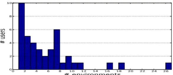
Figure 2. Histogram of the number of environments per user
type of the interface(wireless or wired); and the last tag is the
user tag.
We use a four-tuple composed of the network ID, the network interface, the local ISP, and the local country to identify an environment. In most cases, a pair with the network ID and the network interface is a good identifier for an environment, but there are some exceptions. First, an SSID can be identical across different locations (e.g. coffee shops or hotel chains). Although the BSSID could disambiguate the environments in this case, we do not include it to define an environment because it would also artificially split some unique environments (for instance, when an enterprise or university deploys multiple access points to implement a single network). Second, we observe one user who always use the same device to access the Internet from many different places (i.e. we observe a single MAC address for traces uploaded from different ISPs and countries). Adding the local ISP and country ensures that environments in our dataset are uniquely identified.
III. ENVIRONMENTS AND APPLICATIONS
The first characteristic we looked into was how many environments an individual uses. Fig. 2 shows the histogram of the number of distinct environments per HostView user. We see, that among our users, 25% only use a single environment, while 50% use 5 or more. We even observe a number of individuals with very many environments, 12% use 10 or more and one individual actually used 26 environments. Since our goal is to contrast network performance across environments per end-host, we exclude those users, only connecting via one environment, from the remaining analysis.
Next we examined how much time users spend in each of their environments, and the proportion of traffic generated per environment. Our analysis shows that the fraction of time spent per environment varies significantly from one user to another (plots not shown for conciseness), but nevertheless we observed some general trends. First, users have a small set of dominant environments: 24 users spend 80% of their time in less than three environments. Often a user’s "most-used" environment accounts for more than 50% of their time. Second, there is a strong correlation between the time spent per environment and the number of bytes sent and received in that environment (Pearson’s coefficient is above 0.9 for 90% of the users).
We now investigate where the diversity in environments come from; in other words, is this behavior due to users
Table I
EXAMP LE AP P LI CATI ONS
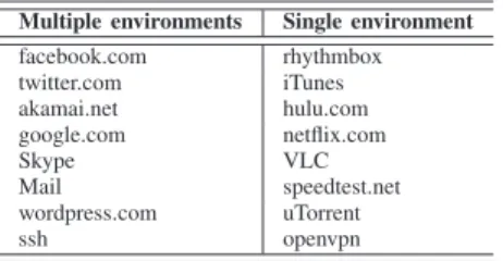
Multiple environments Single environment
facebook.com rhythmbox twitter.com iTunes akamai.net hulu.com google.com netflix.com Skype VLC Mail speedtest.net wordpress.com uTorrent ssh openvpn
employing multiple interfaces or protocols, or due to high mobility such as lot of travel, etc. This can be useful for understanding diversity in network performance; for example, knowing that a user always uses the same network interface, but use numerous source ISPs (or vice versa) might help explain performance differences a user experiences across environments. We found that most of our users connect from only one country, yet up to 75% of the users employee between 2 and 4 ISPs regularly. We do have a few users that connected to 3 or more countries. Most individuals connected to the Internet with ethernet and wireless, but a handful also use ppp, bluetooth, and phone-tethered. Overall, although for roughly 10% of our users, their environment diversity comes from their travel, the main source of diversity for most users is their use of multiple ISPs, and the pairing of a given ISP with either ethernet or wireless.
Another key component influencing the performance in a given environment is the mix of applications used within that environment. Thus we next examine the set of applications used across environments. We use the term single-environment
app to refer to applications that are only used in one envi-ronment, and similarly we use multi-environment app to refer to applications used in multiple environments. Table I lists examples of single-environment and multi-environment appli-cations. The applications included are those that are popular across many users, or else frequently used by some individuals. Many of the popular applications (such as facebook.com and google.com) appear in multiple environments, as expected. There are intuitive hypotheses as to why some of the single-environment applications only occur in one single-environment. For example, video-on-demand and TV applications occur in environments users tag as ’home’; users typically only need openvpn when they are accessing their work network from outside; and speedtest.net is an application users run mainly when they are experiencing problems (which may only occur regularly in one of their environments). Overall, we found that the majority of users (26 out of 30) employ at least 50% of their applications in a single environment. In addition to the reasons cited above (why some applications make sense in a single environment), we note that a number of applications are only used once (such as a web service).
IV. PERFORMANCEACROSSENVIRONMENTS It is interesting to ask whether the same application, or the same set of applications, appearing in two different environ-ments experiences the same or different performance in each
environment. We contrast the performance of a given end-host in two environments by examining both the RTTs and download data rates in each environment. More specifically, we compare the distribution of RTTs in one environment with their distribution in the second environment, and then do the same for download rates. These two metrics capture impor-tant aspects of application performance, including interactive applications (i.e. that need low delay) and bandwidth hungry applications (i.e. that need high data rates). We do this for many pairs of environments using the following methodology.
A. Methodology
We extract RTTs and data rates from network traces using the tcptrace tool. An RTT sample is the time elapsed be-tween the data packet and its corresponding acknowledgment (only for TCP connections). tcptrace does not compute RTTs for retransmitted packets or for delayed or reordered acknowledgments. In our analysis, RTT refers to the average value of RTT samples of a TCP connection over a second.
Download data rate is computed as the total number of unique bytes received by the end-host in one second (i.e., data bytes received excluding retransmitted bytes). We modify tcptrace to generate the data rate per connection in one second bins instead of an average goodput every ten packets or an instantaneous goodput. This yields two time series per network flow, one for RTTs and the other for download rates. We want to compare the distribution of RTTs in two environmentsi and j. Let fiRT T −all(x) denote the empirical
probability distribution that an RTT will take value x in environment i. The superscript RTT-all indicates that the set of RTTs considered are those coming from all applica-tions. Hence our task is to compare the two distributions fRT T −all
i (x) and f
RT T −all
j (x). Similarly we also seek to
compare download rates in 2 environments (i.e.fdown−all i (x)
andfdown−all
j (x)).
To ensure sufficient statistics, we only compare distributions for a given metric if both environments have at least 5000 samples points of the given metric. Hence, this section uses 21 rather than all 30 users, because some users had insufficient data from some environments. If one user has E environments, then we can perform E(E − 1)/2 pairwise comparisons for that user. In total, the number of pairs of environments is 164 for download rates and 112 pairs for RTTs. The reason that we have different numbers of pairs of environments for each metric is because in a single environment we can have an unequal number of samples for download rates and RTTs, depending on what the user is doing.
The statistics literature offers a number of metrics that can be used to compare two distributions, such as the Kol-mogorov–Smirnov (KS), Kullback–Leibler (KL) divergence, and the Hellinger distance. These are typically used as part of a hypothesis test to determine whether or not two distributions are similar. We decided not to use a KS test because it returns the maximum vertical distance between two distributions; this is not suitable for our data since we can have gaps in some ranges of the performance metric for an environment. (This
4
1 Kbit/s 100 Kbit/s 1 Mbit/s 30 Mbit/s
Downlink data rates
0.0 0.2 0.4 0.6 0.8 1.0
CDF
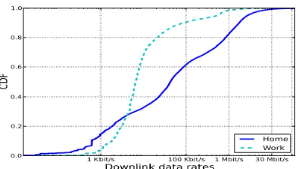
Home WorkFigure 3. Download rates for two environments: HDijdown= 0.38.
occurs since some environments are more used than others and because the mix of applications can be environment dependent.) Moreover the KS test assumes the underlying distributions are continuous. We also decided not to use the KL distance since it is asymmetric (i.e., the results betweeni andj are different than j and i) and because it is unbounded thus making it harder to interpret. Instead we elected to use the a discrete version of the Hellinger distance (HD) [2] that captures the area between two distributions and the difference in shape of two probability mass functions. The HD is computed from two empirical densitiesp(x) and q(x) as follows: HD(p, q) = s 1 − X x∈X pp(x)q(x). (1)
When we apply this to RTT distributions in environments i and j, we have p(x) = fRT T −all
i (x) and q(x) =
fRT T −all
j (x). Let HD RT T −all
ij denote the Hellinger distance
between fiRT T −all(x) and f
RT T −all
j (x). The HD is
sym-metric and bounded in [0,1] where HD = 0 means the distributions are the same and HD = 1 is the maximum divergence between two distributions.
It is always challenging to select a threshold for rejecting the null hypothesis that two distributions are similar. We followed a classical bootstrapping procedure [5] to identify a threshold that would correspond to a value of 0.05 and 0.1 (typical P-values for rejecting the null hypothesis). Our bootstrapping procedure revealed that comparisons across data partitions coming from the same distribution have HD values less than 0.05. However we found that using this procedure we almost always rejected the hypothesis and thus this isn’t useful for our task at hand. (As is well known, statistics is mainly an art form.) We seek to understand when the performance across environments is different and our subsequent work is based on these cases. In order not to exaggerate, we are conservative in our reporting if we underestimate the number of environments that are deemed different. Hence we slightly increase the threshold value used (0.1) to decide if two environments are deemed different. Thus if HDij > 0.1 we consider fi and
fj different. We performed visual inspection of hundreds of
pairs of histograms and found that with a threshold of 0.3, the two distributions were clearly vastly different. In these cases the distributions are "significantly" different because
either the mass of one distribution is largely shifted or the shape of the distribution is completely different. We provide a single illustrative example in Fig. 3. We thus identify three ranges to quantitatively describe the difference between two histogramsfiandfj(we omit the superscript when the context
is clear). If HDij ≤ 0.1 we consider fi and fj similar;
when 0.1 < HDi,j ≤0.3, then fi and fj are different, and
if HDi,j > 0.3, then fi and fj are significantly different.
Although 0.3 is a heuristic, we consider it safe because it is conservative based upon our bootstrapping experiments.
B. Results
We computed HDRT T −allij and HD
down−all
ij for all pairs
i, j for all users. We plot the cumulative distribution of all these values (with one curve per performance metric) in Fig. 4(a). We see that approximately 60% of all environment pairs have a Hellinger distance greater than 0.3 for both RTTs and data rates. This result means that in most cases the distribution of delays and data rates that a host experiences dif-fers significantly across environments. These large differences happen for the vast majority of users: 17 out of 21 users have at least one pair of environments with HDijdown−all > 0.3;
this number is 20 out of 21 for RTTs.
The RTT and download data in Fig. 4(a) comes from all the applications in a given environment, however we observed in Sec. 3 that the mix of applications across environments often differs as there are a number of single-environment ap-plications. The different application mix would explain at least some of the performance differences across environments. In order to understand whether or not performance differences are dominated by environment factors (i.e., the ISP, network interface, country, etc.) rather than the application mix, we extract the set of common applications for all environment pairs. We can then contrast the performance of a pair of environments using performance data (RTTs and download rates) generated only by these common applications. The HDs for RTTs in a pair of environments that includes only the RTTs generated by the common applications are denoted by HDRT T −com
ij . (Similarly we computeHD
down−com ij .)
These modified HD scores are shown in Fig. 4(b). We see that the difference between environments is less pronounced for download data rates when considering only common applications. For example we saw that 64% of environment pairs differed significantly (Fig. 4(a)) when considering all applications, whereas we only 27% of environment pairs exhibit significant difference when considering only common applications. Since the only difference between the experiment in Fig. 4(a) and that in Fig. 4(b) is the inclusion/exclusion (respectively) of single-environment apps, these graphs sug-gest that the application mix (including the single-environment apps) has a stronger influence on the data rates than the environmental factors. However the results are different for RTT behavior. In comparing these two experiments, we find that 64% of environment pairs differ significantly when all applications are considered, and similarly 63% of environment pairs differ significantly when considering common
applica-0.0 0.1 0.2 0.3 0.4 0.5 0.6 0.7 0.8 0.9 Hellinger distance 0.0 0.1 0.2 0.3 0.4 0.5 0.6 0.7 0.8 0.9
CDF
of
env
iron
me
nt p
airs
RTTDownlink data rates
(a) All apps
0.0 0.1 0.2 0.3 0.4 0.5 0.6 0.7 0.8 0.9 Hellinger distance 0.0 0.1 0.2 0.3 0.4 0.5 0.6 0.7 0.8 0.9
CDF
of
env
iron
me
nt p
airs
RTTDownlink data rates
(b) Common apps Figure 4. Distribution of Hellinger distance scores between pairs of network environments.
tions. Thus the application mix is less influential in explaining the significant difference in RTT behaviors across pairs of environments. It thus appears that the environmental factors have a stronger influence on delays than the application mix.
V. RELATEDWORK
We focus our discussion on studies based on passive mea-surements of network traffic and structure it according to the measurement vantage point.
In-network measurements. Zhang et al. [6] developed
a tool T-RAT to breakdown the factors (e.g. congestion, receiver/sender window, bandwidth, short transfers) that limit the data rates achieved by individual TCP connections. A more recent analysis of network traces collected in an ISP network found that TCP data rates are often limited by the application itself, and not the network [7]. Our analysis of data collected on end-hosts confirms that applications often limit achieved data rates, but we also identify a considerable number of instances when the environment limits data rates.
End-host measurements. Before HostView [1], there have
been few efforts to collect data on end-hosts [8]–[10]. A characterization study of enterprise traces [11] analyzed the lifetime of environments (where environment is defined as inside and outside the enterprise) and some network behavior (e.g number of TCP/UDP connections). This study does not analyze the performance metrics we study here and how they vary across environments. Our initial analysis of HostView data studied seven performance metrics only on few instances when users report that performance is poor [12]. Here, we focus on two performance metrics, but we perform a longi-tudinal study of how these metrics vary across environments and applications.
VI. CONCLUSION
In this paper we look at the characteristics and performance of the numerous environments users employ to connect to the Internet. Factors such as the network interface, source ISP, country and user tags differentiate particular environments. We found that users connect to the Internet via many environments (with many people using 4 to 10, and some even higher). We then examined how groups of applications perform, in terms of delay and data rates, in pairs of environments. We observed
that the end-host as a whole (including all applications) typically experiences statistically significant performance dif-ferences in two environments employed a single user. Based on our initial experiments, it appears that the application mix has a stronger influencer on data rates than environmental factors, whereas the reverse is true for round trip time behaviors.
Acknowledgements. This work was supported by the
European Community’s Seventh Framework Programme (FP7/2007-2013) grant no. 258378 (FIGARO) and the Agence National de la Recherche grant C’MON.
REFERENCES
[1] D. Joumblatt, R. Teixeira, J. Chandrashekar, and N. Taft, “Hostview: Annotating end-host performance measurements with user feedback,” in
Hotmetrics, 2010.
[2] G. L. Yang and L. M. L. Cam, Asymptotics in Statistics: Some Basic
Concepts. Berlin: Springer, 2000. [3] D. Joumblatt. http://cmon.lip6.fr/EMD.
[4] F. Gringoli, L. Salgarelli, M. Dusi, N. Cascarano, F. Risso, and K. Claffy, “Gt: picking up the truth from the ground for internet traffic,” in ACM
SIGCOMM CCR, 2009.
[5] M. M. B. Tariq, A. Dhamdhere, C. Dovrolis, and M. Ammar, “Poisson versus periodic path probing (or, does pasta matter,” in In Proc. of
Internet Measurements Conference, 2005.
[6] Y. Zhang, L. Breslau, V. Paxson, and S. Shenker, “On the characteristics and origins of internet flow rates,” in In ACM SIGCOMM, pp. 309–322, 2002.
[7] M. Siekkinen, G. Urvoy-keller, E. W. Biersack, and D. Collange, “A root cause analysis toolkit for tcp,” Computer Networks and Isdn Systems, vol. 52, pp. 1846–1858, 2008.
[8] C. R. Simpson, Jr, D. Reddy, and G. F. Riley, “Empirical models of end-user network behavior from neti@home data analysis,” Simulation, vol. 84, pp. 557–571, October 2008.
[9] E. Cooke, R. Mortier, A. Donnelly, P. Barham, and R. Isaacs, “Reclaim-ing Network-wide Visibility Us“Reclaim-ing Ubiquitous Endsystem Monitors,” in
Usenix Technical Conference, 2006.
[10] S. Guha, J. Chandrashekar, N. Taft, and D. Papagiannaki, “How Healthy are Todayís Enterprise Networks?,” in Proc. f the Internet Measurement
Conference, October 2008.
[11] F. Giroire, J. Chandrashekar, G. Iannaccone, K. Papagiannaki, E. Schooler, and N. Taft, “The cubicle vs. the coffee shop: Behavioral modes in enterprise end-users,” Passive and Active Measurement (PAM)
Conference, 2008.
[12] D. Joumblatt, R. Teixeira, J. Chandrashekar, and N. Taft, “Performance of Networked Applications: The Challenges in Capturing the User’s Perception,” in ACM SIGCOMM Workshop on Measurements Up the