Lagrangian relaxation based heuristic for an integrated production and maintenance planning problem

HAL Id: hal-02111855

https://hal.archives-ouvertes.fr/hal-02111855

HAL is a multi-disciplinary open access archive for the deposit and dissemination of sci-entific research documents, whether they are pub-lished or not. The documents may come from teaching and research institutions in France or abroad, or from public or private research centers.

L’archive ouverte pluridisciplinaire HAL, est destinée au dépôt et à la diffusion de documents scientifiques de niveau recherche, publiés ou non, émanant des établissements d’enseignement et de recherche français ou étrangers, des laboratoires publics ou privés.

Lagrangian relaxation based heuristic for an integrated

production and maintenance planning problem

Marouane Alaoui-Selsouli, Abdelmoula Mohafid, Najib Najid

To cite this version:

Marouane Alaoui-Selsouli, Abdelmoula Mohafid, Najib Najid. Lagrangian relaxation based heuris-tic for an integrated production and maintenance planning problem. International Journal of Pro-duction Research, Taylor & Francis, 2012, 50 (13), pp.3630-3642. �10.1080/00207543.2012.671586�. �hal-02111855�

Lagrangian Relaxation based Heuristic for an Integrated Production

and Maintenance planning Problem.

M. Alaoui-Selsouli, A. Mohafid*, N.M. Najib

Marouane Alaoui-Selsouli

IRCCyN\ Ecole des Mines de Nantes

4, rue Alfred Kastler, B.P. 20722F-44307 Nantes cedex France. Email : malaou07@mines-nantes.fr

Tel. 00 33 2 28 09 21 17, Fax. 00 33 2 28 09 20 21

*Abdelmoula Mohafid

Université de Nantes, Nantes Atlantique, IRCCyN

IUT de Nantes, Dep. QLIO. 2, avenue du Prof Jean Rouxel, B.P. 539- 44475 Carquefou, France.

Email: abdelmoula.mohafid@univ-nantes.fr Tel: +33 2 28 09 21 06, Fax: +33 2 28 09 20 21

Najib .M. Najid

Université de Nantes, Nantes Atlantique, IRCCyN

IUT de Nantes, Dep. GMP.2, avenue du Prof Jean Rouxel, B.P. 539- 44475 Carquefou, France.

Email : najib.najid@univ-nantes.fr

Tel : +33 2 28 09 20 94, Fax. +33 2 28 09 20 21

Abstract: In this paper, an approach is developed to solve the joint production planning and maintenance problem. Moreover, some propositions and mathematical properties were suggested and applied in the proposed heuristic to solve this integrated problem. It is based on Lagrangian relaxation (Fisher 1981) of the capacity constraints and sub-gradient optimization. At every step of sub-gradient method, a smoothing procedure is applied to the solution of the Lagrangian problem to ensure the feasibility of solution and to improve it. Computational experiments are carried out to show the results obtained by our approaches and are compared to those of a commercial solver.

Keywords: Production, Maintenance, Integer Programming, Time Windows, Shortage, Heuristics.

1.

Introduction

Maintenance is a task closely related to production scheduling in industrial settings. It is the

function that allows maintaining or restoring equipment to a specific state and guaranteeing a

given service. Production and maintenance activities conflict since maintenance is generally

considered as a secondary process in companies that have production as their core business.

Indeed, preventive maintenance activities are often carried out in hours or days out of service.

Therefore, the number of breakdowns increases and the availability of production equipment

is reduced. We can notice then that production planning and maintenance are addressed

separately in the literature and also in the industry. As a remedy to this problem, the

maintenance planning should be an integral part of the overall business strategy and should be

coordinated and scheduled with manufacturing activities. So, maintenance should be

considered as integral parts of the production plan rather than as interruptions to that plan and

any violation of the maintenance schedule will induce a violation of the production plan

integrity.

In this paper, a new integrated production and maintenance planning problem is studied

considering a single production line at the tactical level. For production planning, the single

stage multi item capacitated lot sizing problem with demand shortages is proposed. The

objective is to determine the schedules and lot sizes of multiple items that share capacity

constraint resources. The problems deals with tight capacities and when the capacity is

insufficient to produce the total demand, it is spread among the items by minimizing the total

amount of demand shortages. The maintenance planning problem is to determine the dates of

preventive maintenance in time windows according to reliability of production equipment and

demand. When preventive maintenance actions are carried out the production line is restored

to as good as new (AGAN) state, i.e. the system has the same lifetime distribution and failure

performed to restore the system to the failure rate it had when it failed (as bad as old (ABAO)

state). The resulting problem is modeled as a linear mixed-integer program to minimize

production, inventory, setup, demand shortage, preventive and corrective maintenance costs.

To our knowledge, there are only few works dealing with this issue. An integrated aggregate

production planning and maintenance problem was tackled initially by Weinstein and Chung

(Weinstein and Chung, 1999). The authors presented a three part-model to solve the

conflicting objectives of system reliability and profit maximization. An aggregate production

plan is first generated, and then a master production schedule is developed to minimize the

weighted deviations from the specified aggregate production goals. Finally, work-center

loading requirements, determined through rough cut capacity planning, are used to simulate

equipment failures during the aggregate planning horizon. Unlike Weinstein and Chung,

Aghezzaf et al (Aghezzaf et al. 2007) proposed an integrated aggregate production planning

and maintenance model for a system that is periodically renewed and minimally repaired at

failure. They assumed that any maintenance action carried out on the system in a given period reduces the system’s available production capacity during that period. The objective was to find an integrated lot-sizing and preventive maintenance strategy of the system that satisfies

the demand for all items over the entire horizon without backlogging, and which minimizes

the expected sum of production and maintenance costs. An extension of the above work is

treated by Aghezzaf and Najid (Aghezzaf and Najid, 2008) by considering parallel production

lines. Recently, we treated the problem of integrating production and maintenance for small

instances in (Najid et al. 2010). The integrated model and the separate model (where

production and maintenance are planned separately) were solved and a comparison between

integrated and separate models was studied and showed the effectiveness of the integrated

one. Nourelfath et al. (Nourelfath et al. 2010) integrated preventive maintenance with tactical

lot-sizing and preventive maintenance strategy of the system that will minimize the sum of

maintenance, setup, holding, backorder, and production costs, while satisfying the demand for

all products over the entire horizon.

While all above mentioned papers consider that preventive maintenance activities should be

planned at a fixed date, the present work provides more flexibility to preventive maintenance

tasks with time windows to better optimize the overall cost of production and maintenance.

The remainder of the paper is organized as follows. In the second section, the description and

mathematical formulation of the problem are presented. The heuristics to solve the integrated

problem are developed in the third section and some computational results are showed in the

fourth section. Finally, we end up with conclusion and prospects in the last section.

2.

Mathematical model

2.1 Preventive Maintenance Policy

Our preventive maintenance (PM) policy is planned in time windows and based on the

periodic PM policy, see e.g. (Barlow and Hunter, 1960), Nakagawa (Nakagawa 1981a, b),

Wang and Pham (Wang and Pham, 1999). In the classical periodic PM policy, the equipment

is maintained at fixed time intervals (k=1, 2…) where ( is the

optimal number of PM period and is the length of each period t H) is the optimal length of PM period. Therefore, PM tasks will be performed periodically in the beginning of period’s t =1, +1, 2 +1, 3 +1, +1 etc. In our study, The PM actions are planned in time

windows where and is the number of

preventive maintenance activities during the horizon, and is defined as:

Thus, a preventive maintenance task will be carried out at the earliest in the beginning of the

complete within the period in which it started. The parameter k which determines the width of

the time windows is chosen to avoid their overlapping:

Moreover, we assume that each preventive or corrective maintenance action carried out on the

production line consumes capacity units and at the beginning of the planning horizon the

production line is considered as new. When a preventive maintenance is planned, the

production line is restored to AGAN state and when a production line fails, a minimal repair is performed to restore it to “as bad as old” (ABAO) state. The production line is considered here as a complex system and the failure rate is an overall rate of the whole line. It is also

assumed that the failure distribution of the production line is known. Let and denote

its corresponding probability density and cumulative distribution functions, respectively. Let

denotes the failure rate function of the production line at time .

Finally, we assume that expected failures increase with elapsed time since the last preventive

maintenance.

The objective of the maintenance problem is to decide when performing preventive

maintenance activities in predetermined time windows and reducing the number of failures.

The expected maintenance cost during the horizon is defined as the sum of preventive and

corrective maintenance costs.

2.2 Planning Time windows

To determine time windows, we need to estimate, for each period t of the horizon, the

expected number of failures, denoted essential to compute the expected maintenance

The optimal length of preventive maintenance period corresponds to the period

t which minimizes the expected maintenance cost per unit time, denoted CM(t), and given by :

Where and are respectively preventive and corrective maintenance costs, and is the

expected maintenance cost during [0, t] and given by:

Example:

If we consider an horizon with 9 periods and an optimal length of preventive maintenance

period ( ), the maintenance planning, without considering production

constraints, is shown in figure 1. By using equation (2), k is equal to 1 and then time windows

in the whole of horizon are defined as shown in figure 2

[Figures 1, 2]

2.3 Integrated production and maintenance planning model

The studied problem is an integrated production and maintenance planning model where

preventive maintenance activities are carried out in time windows. The production planning

considers a planning horizon H of length covering N periods of fixed length ,

and a set of items to be produced on a single capacitated production line. During each

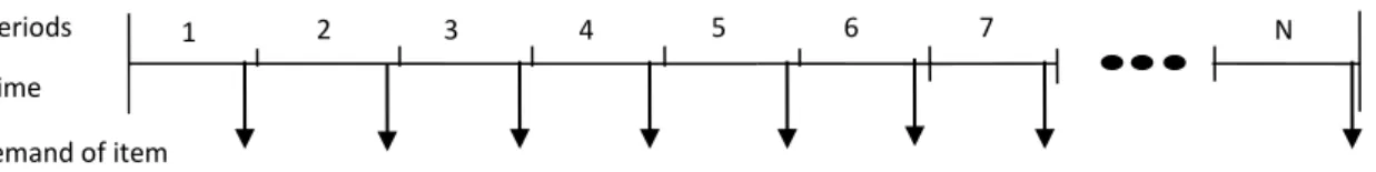
period , a demand of the item should be satisfied (figure 3). Items are produced

on a production line with known capacities given in unit time, and processing time is

expressed in unit time per item. Furthermore, the demand shortage is allowed to be unfulfilled

due to insufficient capacity and using a high unit cost for each item lost.

[Figure 3]

Index:

i: Items. t: Periods.

Parameters:

: Demand of item i to satisfy during period t. K (t) : Available capacity in period t.

: Set-up cost of producing one unit of item i in period t. : Fixed cost of producing one unit of item i period t.

: Variable cost of holding one unit of item i by the end of period t. : Unit cost for demand shortage of item i in period t.

: Expected maintenance cost when preventive maintenance task is carried out in period t.

: Processing time for each item i.

) : Expected capacity consumed by each preventive maintenance action in period t. (t) : Expected capacity consumed by each corrective maintenance action in period t.

: Expected capacity consumed by maintenance when preventive maintenance task is carried out in period t.

: Vector of N elements contains the expected number of failures in each period t, when no preventive maintenance task is performed.

= [NB(1), NB(2), NB(3)… NB(T)]

Decision variables:

: Binary set-up variable of item i in period t. : Quantity of item i produced in period t. : Inventory of item i at the end of period t. : Demand shortage for item i in period t.

: Binary preventive maintenance variable (1 if preventive maintenance is carried out in the beginning of period t, 0 otherwise).

: Binary variable (1 if in period t the last preventive maintenance ended in period j, 0 otherwise).

Subject to:

The objective function (7) minimizes the sum of the set-up, holding, production, demand

shortage, and maintenance (preventive and corrective) costs over the whole N-periods

capacity constraints that consider preventive and corrective maintenance. Indeed, if a

preventive or corrective maintenance activity is carried out, a part of the available capacity is

consumed. Constraint (10) relates the continuous production variables to the binary setup

variables. Constraint (11) expresses that quantity lost of item i in period t must be less than or

equal to demand of item in period t. Constraint (12) ensures that one maintenance must

be carried out in the interval . Constraint (13) ensures that two

preventive maintenance actions cannot be carried out in successive time periods. Constraints

(14)-(16) force variable to 1 if, in period t, the last preventive maintenance ended in period

j, 0 otherwise. Those constraints are equivalent to .

Constraints (17)-(20) express non-negativity and integrality constraints.

2.3 Evaluation of and

When preventive maintenance activities are performed in period t, the expected cost generated

and the capacity consumed by maintenance, are, respectively, and . The

maintenance cost in this period t is the sum of preventive and corrective maintenance costs.

The corrective maintenance cost in period t is the product of the expected number of failures

and the corrective maintenance action cost in the same period. Thus, the expected

maintenance cost in each preventive maintenance period t is:

The same reasoning can be applied for the capacity consumed by maintenance task in a

Notice that if no preventive maintenance action is performed, the expected maintenance cost

and the capacity consumed in period t are, respectively, the expected cost generated and the

capacity consumed by corrective maintenance:

With j is the period where the last preventive maintenance activity was performed.

3.

Heuristic for ULSP-TW-SC

In our decomposition method, the integrated production and maintenance problem is divided

into a set of sub-problems. Each sub-problem is a single item uncapacitated lot sizing problem

with time windows and shortage cost called ULSP-TW-SC. This sub-problem is a combination

of the single item capacitated lot sizing problem with shortage cost (ULSP-SC) treated by

Aksen et al (Aksen et al, 2003) solved in and a maintenance problem where preventive

maintenance tasks are planned in time windows.

Subject to:

(8) - (24) excepting capacity constraints (9.1) and (9.2).

The solution of the problem (ULSP-TW-SC) was carried out by using the optimization solver

"XpressMP" and the results showed that the computation time increases exponentially when

The numerical tests were performed on a computer with an Intel Core Duo 2.13 GHz and 4

GB of memory. For each planning horizon length such that 0 ≤ N ≤ 150, we

generated 10 problems randomly. The demand shortage costs are selected between 30 and 100

and the demand in each period of the horizon is chosen in the interval [20.100]. The

average computation time needed to solve these problems is given in Table 1. These results

are also shown graphically in Figure 4. Note the exponential growth of computing time from

N = 70.

[Table 1] and [Figure 4]

To solve the problem (ULSP-TW-SC), a heuristic based on a dynamic programming

algorithm proposed by Aksen et al. (Aksen et al. 2003) is developed. The expected gap

between the optimal solution (or a lower bound) obtained by the solver and the one provided

by the heuristic is equal to 0.113%. The main steps of this heuristic are described below:

Step 1: Solve the single item Uncapacitated Lot Sizing Problem with Shortage Cost

(ULSP-SC) to optimality using the dynamic algorithm addressed by Aksen et al (Aksen et al, 2003)

and based on the structural characteristics stated in lemmas 1 to 3.

Lemma 1:

Under assumption that , the first lemma suggests that there is an optimal solution such

that demand in a given period will be fully satisfied if procurement is made in that period.

Lemma 2:

The second lemma suggests that there is an optimal solution such that we will procure in a

given period only if the inventory level at the end of the preceding period drops to zero. This

(Wagner et Whitin, 1958), according to which beginning inventory in a period of procurement

activity is always zero. In our lost demand model, it is slightly altered such that we might

have both and if the demand is not met.

Lemma 3:

The third lemma suggests that there is an optimal solution such that if we lose any demand in

a given period, then we should lose the entire demand in that period. In other words, it

prohibits partial loss of demand. If , then must equal .

The proofs of the lemmas 1 to 3 can be found in (Aksen et al. 2003).

Step 2: Select the first time window, plan a preventive maintenance task in the period when

the total cost of production and Maintenance is minimal.

Step 3: Update the total cost of production and maintenance, select the next time window and

plan a preventive maintenance task in the period when the total cost is minimal.

4.

Heuristic based on Lagrangian relaxation (LH)

Our heuristic is based on the Lagrangian relaxation approach. The general idea is to

decompose our integrated production planning and maintenance problem to N sub-problems

easy to solve by relaxing the resource capacity constraints (10) and by using a set of Lagrange

multipliers in the objective function of the MCLSP-TW-SC model.

Let the Lagrangian function, the mathematical formulation of relaxed

problem (MULSP-SC-TW) is stated below:

Subject to:

(27)

(8) - (24) excepting capacity constraints (9.1) and (9.2).

The Lagrangian relaxation of the capacity constraints of the MCLSP-TW-SC decomposes the

model into n single-item uncapacitated lot-sizing problems with shortage cost and time

windows, denoted ULSP-TW-SC and solved in section 3.

From Lagrangian relaxation theory (Fisher, 1981), is a lower bound of the

optimal solution of MCLSP-TW-SC. The greatest lower bound attainable with the Lagrangian

relaxation is provided by multipliers obtained by solving the following Lagrangian dual

problem (LD) which can be solved efficiently by a sub-gradient optimization procedure

(Fisher, 1981).

Subject to:

The main advantage of using a Lagrangian relaxation is that it usually preserves most of the

original problem structure. This makes it easier to use the relaxed problem solution to

generate a feasible solution for the original problem. Therefore, a very efficient heuristic

procedure and by checking, at each iteration, if the solution provided by the primal sub

problem is a feasible solution of MCLSP-TW-SC, i.e. if

, then this solution is optimal. Otherwise, this solution can

be modified by using a perturbation procedure (smoothing procedure) to generate a feasible

solution for MCLSP- TW-SC. A detailed heuristic based on this idea is presented in the

following subsection.

4.1 Lagrangian heuristic algorithm

Our overall solution method to solve MCLSP-TW-SC is a modified sub-gradient optimization

procedure. At a given iteration, if the Lagrangian solution is not feasible for MCLSP-SC-TW,

this solution is modified using the heuristic described in following sub-section 4.2 to find a

new feasible solution for MCLSP-TW-SC, if its value is better than the current upper bound,

it becomes the new one. The Lagrangian multipliers are initially set to zero and updated on

each iteration to maximize the objective function of dual relaxed problem (LD) according to

the formula:

:= max (0, + ),

Where is the sub-gradient of given by:

.

is the norm of the sub-gradient vector and is the sub-gradient step size:

, we start with and divide by 2 if any improvement of is seen

after some iterations. Finally, the stopping criterion is based on maximum number of

iterations or when the Gap between upper and lower bounds is smaller than a value . A

detailed description of the Lagrangian heuristic is found below:

1. Initialization:

t= 1, 2…T. (Lagrange multipliers) k =1 (Iteration counter)

(Multipliers)

(Lower bound value)

(Upper bound value where M is a large number)

2. For a given iteration k:

(a) Solving the Lagrangian problem with .

If Lagrangian solution is feasible then

Stop the algorithm.

(b) Compute the new lower bound:

If > then

(c) Perturbation procedure: a heuristic is used to find a feasible solution using a

smoothing procedure as described in the following sub-section 4.2.

If < then

(d) Compute sub-gradient of .

(e) Compute sub-gradient step size .

(f) Updating Lagrange multipliers .

If (no improvement after more than K iterations) then : = 2 Else : =

(g) Stopping criteria:

- Maximum number of iterations is reached. - Or when Gap is less than a value ( > 0).

4.2 Smoothing Procedure

In order to find a feasible solution at each step of the Lagrangian relaxation, we propose a

procedure to provide an upper bound, denoted NAM. It is based on the Lagrangian solution

obtained at each step of the Lagrangian heuristic algorithm. Since the capacity constraints

(9.1) and (9.2) are relaxed, the Lagrangian solution violates them. The NAM heuristic is

mainly based on a smoothing procedure to lower shortages by reusing missing resource

capacities. The heuristic is based on the work of Trigeiro et al. (Trigeiro et al., 1989) who

proposed an efficient Lagrangian relaxation heuristic for the classical multi-item capacitated

lot sizing problem with setup times. Recently, Brahimi et al (Brahimi et al. 2006) proposed a

generalization of Trigeiro et al (Trigeiro et al, 1989) smoothing heuristic to solve the

multi-item capacitated lot sizing problem with time windows. Notice that the NAM procedure uses

the Propositions 5 and 6 and the formula below, that computes the overtimes in each period,

to find a feasible solution and to improve it.

Proposition 5: From the solution obtained by solving the Lagrangian problem, if in period t

and for l = {1 ... j-1}, then a set-up of production has been performed in

period t and the next setup was planned in period t + j, therefore:

and for

Proof

At each iteration of the algorithm 2, the relaxed problem of (MCLSP-TW-SC) is solved. If we

notice that and for then there was unavoidably the setup of

one or several items in the period t.

According to lemma 2, we never produce in a period when the inventory level of a previous

period is non-zero, i.e. In our case, an amount of one or several

references was produced in the period t ( ) as the overtimes are greater than zero

( ). Moreover, since for we can deduce that one or several items have not been produced between period’s t+1 and t+j-1 and that their demands were met by the inventory built in the period t, so .

and for

and for

Our NAM procedure is described as follows:

Step1: After solving the relaxed problem, several cases arise. According to Proposition 5, the

surplus amounts produced are shifted from period t to period t+1 using Proposition 2 (see

section 4.1.2).

Step2: in some periods, if and the quantity of one or several items is lost, then the

demand shortage should be shifted to a quantity produced in the current period according to

Proposition 3 (see section 4.1.2).

Step 3: From the solution obtained by steps 1 and 2, if, at a given period, and

, a quantity of one or several items produced in period t+1 is shifted to the previous

Step4: After the step 3, we must verify that, in each period, the available capacity is not

exceeded. Otherwise, if at a given period, and such , a quantity of one or

several items is selected to be lost in the same period according to Proposition 4 (section

4.1.2). Else if and such , the quantity lost of one or several items in period t+1 will be a quantity produced in period t according to Proposition 4.

5.

Computational results

In this section, we present different tests resulting from the application of the Lagrangian

heuristic, denoted (LH). Our algorithms were implemented in the Java programming

language. The computations were tested on an Intel Core 2 CPU 2.2GHz PC with 4GB RAM.

Computational tests are performed on a series of extended instances from the lot-sizing library

LOTSIZELIB, initially described in (Trigeiro et al. 1989). These instances are denoted by

trn−N, where n = 6, 12, 24 is the number of items and N = 15, 30 is the number of periods.

These instances are characterized by variable resource consumption equal to one, and enough

capacity to satisfy all demands over the planning horizon. They are also characterized by

important setup costs, small setup times. Since these instances have enough capacity to satisfy

all demands over the planning horizon, some modifications were made to induce shortages.

A planning horizon composed of N production periods of fixed length is considered to

produce a set of items on the production line with an available capacity. The production,

set-up, and holding costs are, respectively, 10, 30, and 5. Four parameters are considered for the

analysis:

Problem dimension: The problem dimensions represented by the number of items n

and the number of periods N = 15 and 30.

Production capacity: The capacity required, in each period, is initially computed as

the target average utilization of capacity . The factor is set to 0.95 and 1.1 corresponding

respectively to situations with tight and too tight capacity constraints.

Demand pattern: The demand for each item in each period is generated randomly on the

interval [20,100].

Shortage cost: the shortage cost is considered as penalty cost and its value for each item is

generated from the follows intervals [I1], [I2] and [I3].

 [I1]: [0.5*(Production cost+ setup cost), 1.5*(Production cost+ setup cost) ]  [I2]: [0.5*(Production cost+ setup cost), 2.5*(Production cost+ setup cost) ]  [I3]: [0.5*(Production cost+ setup cost), 3.5*(Production cost+ setup cost) ] Six classes of instances are created:

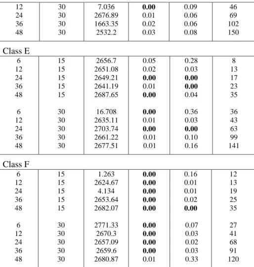
 Class A, Class B and Class C: Too tight capacity and shortage cost for each item is generated from [I1], [I2] and [I3], respectively.

 Class D, Class E and Class F: Tight capacity and shortage cost for each item is generated from [I1], [I2] and [I3], respectively.

All problem tests are generated with Weibull distribution of production line. The shape and

scale parameters are respectively , and . The cost of preventive maintenance action

is set to , and the cost of minimal repair action is given by . The capacity lost

when a preventive maintenance task and minimal repair action are carried out, is

respectively and . Table 2 shows the expected number of

failures in each period NB(t) as a function of system’s age.

We assume that the system lifetime is distributed according to weibull distribution with

[Table 2]

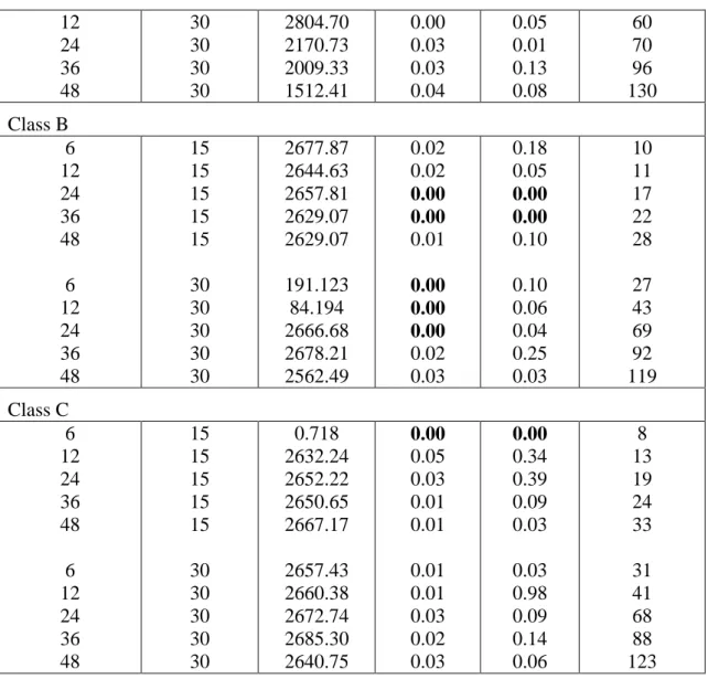
To have a meaningful comparison, we compare the results of the lagrangian heuristic to those

obtained by XpressMP solver. The computational results of the heuristic (LH) and the solver

are shown in Tables 3 and 4. The gaps between the best lower bounds or optimal solution

obtained and the upper bounds provided by the heuristics and by the solver are computed

respectively by the given formula suggested by Millar and Yang (1994): The different gaps

are expressed using equations (28) and (29).

The stopping criterion of the XpressMP computation is a time limit equal to 3600 seconds or

when the gap reaches a minimal value ( ). For the Lagrangian heuristic, it is when a

number of sub-gradient iteration reaches a maximum of iteration and also if the gap is

small than .

[Table 3]

Tables 3 and 4 summarize the computational behavior of the Lagrangian heuristic and the

computational results given by the solver. The gaps and CPU time are computed for each

instance with the following parameters: the number of items (n), the number of periods (N),

shortage cost for each item and capacity tightness.

The results obtained with solver are very interesting. Indeed, most of instances are solved to

optimality or are very close to optimal solution, but also require a significant amount of CPU

quality solution. Then, a heuristic based on lagrangian relaxation (LH) is implemented. The

results provided by (LH) are shown in Table 3 when capacity is too tight and in Table 4 when

capacity is larger (tight capacity).

[Table 4]

We notice from Tables 3 and 4 that the heuristic LH can solve some instances to optimality.

Others instances, which are not solved to optimality, have very small gaps and the upper

bounds of the Lagrangian heuristic are very close to the upper bounds obtained by the solver and the deviation from the solver doesn’t exceed 0.97%. Also, we can observe that the CPU time of the Lagrangian heuristic enhance partially when we increase the number of items and

considerably when we increase the number of periods. Finally, the computation time of the

heuristic is much smaller than that of the solver for the same or a close result.

6.

Conclusion and perspectives

We have formulated a mixed-integer linear programming model to plan jointly production

and maintenance activities. The model takes into account the reliability (expected number of

failures) production and maintenance costs, and demand shortage. Preventive maintenance is

carried out in pre-determined time windows, and corrective maintenance is performed to

restore the system to an operating state without changing the failure rate function.

Computation results show that the Lagrangian heuristic (LH) seems a good trade-off between

the solution quality and time execution. Therefore, for a decision maker who is interested in a

good solution quality and a short execution time, our Lagrangian heuristic can be an

appropriate approach to solve the problem.

A Sensitivity Analysis would be a good perspective of this work to study how a change in the

An extension of our model to the concept of imperfect maintenance can be very useful to

model a more realistic and accurate maintenance operations, which are in reality neither

perfect nor minimal.

Finally, other heuristics can be developed and compared to solve our integrated problem in a

reasonable time.

References

Aghezzaf, E.H., Jamali, M.A., and Ait-Kadi, D. (2007). An integrated production and

preventive maintenance planning model. European journal of operational research, 181,

676-685.

Aghezzaf, E.H., and Najid, N.M. (2008). Integrated production and preventive maintenance in

production systems subject to random failures. Information science, 178, 3382-3392.

Barlow, R.E., and Hunter, L.C. (1960). Optimum preventive maintenance policies. Operations

research, 8, 90-100.

Aksen, D., Altinkemer, K., and Chand, S. (2003). The single-item lot-sizing problem with

immediate lost sales. European Journal of Operational Research, 147 (3), 558–566.

Brahimi, N., Dauzère-Pérès, S., and Najid, M.N. (2006). Capacitated multi-item lot-sizing

problems with time windows. Operations Research, 54, 951–967.

Dantzig, G.B., and Wolfe, P. (1960). Decomposition principle for linear programs. Operations

Research, 8, 101–111.

Degraeve, Z., and Jans, R. (2007). A New Dantzig- Wolfe Reformulation and

Branch-and-Price Algorithm for the Capacitated Lot-Sizing Problem with Setup Times. Operations

Dzielinski, B.P., and Gomory, R.E. (1965). Optimal programming of lot sizes, inventory, and

labor allocations. Management Science. 11(9), 874–890.

Jans R., and Degraeve, Z. (2007). Meta-heuristics for dynamic lot sizing: A review and

comparison of solution approaches. European Journal of Operational Research, 177,

1855-1875.

Manne, A.S. (1958). Programming of economic lot-sizes, Management Science, 4, 115–135.

Millar, H.H., and Yang, M. (1994). Lagrangean heuristics for the capacitated multi-item

lot-sizing problem with backordering. International Journal of Production Economics, 34, 1–15.

Najid, M.N, Alaoui-selsouli, M., and Mohafid, A. (2010). An Integrated Production and

Maintenance Planning Model with time windows and shortage cost. International Journal of

Production Research, DOI: 10.1080/00207541003620386.

Nakagawa, T. (1981a). A summary of periodic replacement with minimal repair at failure.

Journal of the Operations Research Society of Japan, 24, 213–228.

Nakagawa, T., (1981b). Modified periodic replacement with minimal repair at failure. IEEE

Transactions on Reliability, 30, 165–168.

Nourelfath, M., Fitouhi, M., and Machani, M. (2010). A genetic algorithm for integrated

production and preventive maintenance planning in multi state systems. IEEE Transactions on

Reliability, 59(3), 496 – 506.

Trigeiro, W., Thomas, L.J., and McLain, J.O. (1989). Capacitated lot sizing with setup time.

Management science, 35, 353-366.

Wagner, H.M., and Whitin, T.M. (1985). A dynamic version of the economic lot size model,

Wang, H. (2002). A survey of maintenance policies of deteriorating systems. European

Journal of Operational Research, 139, 469-489.

Wang H., and Pham, H. (1999). Some maintenance models and availability with imperfect

maintenance in production systems. Annals of Operations Research, 91, 305–318.

Weinstein, L., and Chung, C., (1999). Integrating maintenance and production decisions in a

hierarchical production planning environment. Computers & operations research, 26,

1059-1074.

1 2 3 4 5 6 7 8 Time windows

Figure 2: Time windows of preventive maintenance in integrated case 1 2 3 4 5 6 7 8

Figure 1: Maintenance plan without considering production cost (

Horizon Length Computation time (s) 10 0.031 20 0.125 40 1.123 60 6.97 70 19 80 169 0 500 1000 1500 2000 2500 10 20 30 40 50 60 70 80 100

CPU time (s)

Figure 3 : Production planning

100 442

150 *2238

Solver LH

Items Periods Time (s) Gap1(%) Gap2(%) Time (s) Class A 6 12 24 36 48 6 15 15 15 15 15 30 49.52 226.3 2677.44 2693.89 2641.43 2723.36 0.00 0.00 0.00 0.00 0.00 0.01 0.07 0.09 0.00 0.00 0.01 0.10 9 11 16 25 30 35 Periods Expected number of failures Periods Expected number of failures 1 2 3 4 5 6 7 8 9 10 11 12 13 14 15 0.0157 0.1095 0.2970 0.5782 0.9532 1.4220 1.9845 2.6407 3.3907 4.2345 5.1720 6.2032 7.3282 8.5470 9.8595 16 17 18 19 20 21 22 23 24 25 26 27 28 29 30 11.2657 12.7657 14.3595 16.0470 17.8282 19.7032 21.6720 23.7345 25.8907 28.1407 30.4845 32.9220 35.4532 38.0782 40.7970

Table 2: Expected number of failures

* : Over flow of the solver without obtaining an optimal solution

12 24 36 48 30 30 30 30 2804.70 2170.73 2009.33 1512.41 0.00 0.03 0.03 0.04 0.05 0.01 0.13 0.08 60 70 96 130 Class B 6 12 24 36 48 6 12 24 36 48 15 15 15 15 15 30 30 30 30 30 2677.87 2644.63 2657.81 2629.07 2629.07 191.123 84.194 2666.68 2678.21 2562.49 0.02 0.02 0.00 0.00 0.01 0.00 0.00 0.00 0.02 0.03 0.18 0.05 0.00 0.00 0.10 0.10 0.06 0.04 0.25 0.03 10 11 17 22 28 27 43 69 92 119 Class C 6 12 24 36 48 6 12 24 36 48 15 15 15 15 15 30 30 30 30 30 0.718 2632.24 2652.22 2650.65 2667.17 2657.43 2660.38 2672.74 2685.30 2640.75 0.00 0.05 0.03 0.01 0.01 0.01 0.01 0.03 0.02 0.03 0.00 0.34 0.39 0.09 0.03 0.03 0.98 0.09 0.14 0.06 8 13 19 24 33 31 41 68 88 123 Solver LH

Items Periods Time (s) Gap1(%) Gap2(%) Time (s)

Class D 6 12 24 36 48 6 15 15 15 15 15 30 2666.58 2642.53 2679.54 2658.76 2677.53 1662.35 0.01 0.01 0.00 0.00 0.01 0.00 0.16 0.02 0.00 0.09 0.10 0.10 11 13 18 27 36 27

12 24 36 48 30 30 30 30 7.036 2676.89 1663.35 2532.2 0.00 0.01 0.02 0.03 0.09 0.06 0.06 0.08 46 69 102 150 Class E 6 12 24 36 48 6 12 24 36 48 15 15 15 15 15 30 30 30 30 30 2656.7 2651.08 2649.21 2641.19 2687.65 16.708 2635.11 2703.74 2661.22 2677.51 0.05 0.02 0.00 0.01 0.00 0.00 0.01 0.00 0.01 0.01 0.28 0.03 0.00 0.00 0.04 0.36 0.03 0.00 0.10 0.16 8 13 17 23 35 36 43 63 99 141 Class F 6 12 24 36 48 6 12 24 36 48 15 15 15 15 15 30 30 30 30 30 1.263 2624.67 4.134 2653.64 2682.07 2771.33 2670.3 2657.09 2659.6 2680.87 0.00 0.00 0.00 0.00 0.00 0.00 0.00 0.00 0.00 0.01 0.16 0.01 0.01 0.02 0.00 0.07 0.03 0.02 0.03 0.33 12 13 19 25 35 27 41 68 91 120