HAL Id: hal-02387002
https://hal.archives-ouvertes.fr/hal-02387002
Submitted on 29 Nov 2019
HAL is a multi-disciplinary open access
archive for the deposit and dissemination of
sci-entific research documents, whether they are
pub-lished or not. The documents may come from
teaching and research institutions in France or
abroad, or from public or private research centers.
L’archive ouverte pluridisciplinaire HAL, est
destinée au dépôt et à la diffusion de documents
scientifiques de niveau recherche, publiés ou non,
émanant des établissements d’enseignement et de
recherche français ou étrangers, des laboratoires
publics ou privés.
Comparing the modeling powers of RNN and HMM
Achille Salaün, Yohan Petetin, François Desbouvries
To cite this version:
Achille Salaün, Yohan Petetin, François Desbouvries. Comparing the modeling powers of RNN and
HMM. ICMLA 2019: 18th International Conference on Machine Learning and Applications, Dec 2019,
Boca Raton, FL, United States. pp.1496-1499. �hal-02387002�
Comparing the modeling powers of RNN and HMM
Achille Salaün
∗†, Yohan Petetin
∗, François Desbouvries
∗∗Samovar, CNRS, Telecom SudParis, Institut Polytechnique de Paris (Evry, France)
{yohan.petetin, francois.desbouvries}@telecom-sudparis.eu
†Nokia Bell Labs(Nozay, France)
Abstract—Recurrent Neural Networks (RNN) and Hidden Markov Models (HMM) are popular models for processing sequential data and have found many applications such as speech recognition, time series prediction or machine translation. Although both models have been extended in several ways (eg. Long Short Term Memory and Gated Recurrent Unit architec-tures, Variational RNN, partially observed Markov models. . . ), their theoretical understanding remains partially open. In this context, our approach consists in classifying both models from an information geometry point of view. More precisely, both models can be used for modeling the distribution of a sequence of random observations from a set of latent variables; however, in RNN, the latent variable is deterministically deduced from the current observation and the previous latent variable, while, in HMM, the set of (random) latent variables is a Markov chain. In this paper, we first embed these two generative models into a generative unified model (GUM). We next consider the subclass of GUM models which yield a stationary Gaussian observations probability distribution function (pdf). Such pdf are characterized by their covariance sequence; we show that the GUM model can produce any stationary Gaussian distribution with geometrical covariance structure. We finally discuss about the modeling power of the HMM and RNN submodels, via their associated observations pdf: some observations pdf can be modeled by a RNN, but not by an HMM, and vice versa; some can be produced by both structures, up to a re-parameterization. Index Terms—Recurrent neural networks, Hidden Markov Models
I. INTRODUCTION
Let us consider the general time series prediction prob-lem, which consists in predicting random future observations {Xt+1, · · · , Xt+j} = Xt+1:j from a realization of the past
ones, {x0, · · · , xt} = x0:t∈ Rt+1.
This problem has many applications such as speech recogni-tion [6] [12], time series predicrecogni-tion [8], or machine translarecogni-tion [3]. Various tools have been proposed to address this problem [14]. In particular, a solution to such a prediction problem is brought by generative models. Such models aim at modeling the observation sequence with a probability distribution pθ(x0:t),
where θ describes the set of parameters of the corresponding generative model. Once the model is known (i.e. θ has been estimated), the prediction of the future observations is computed from pθ(xt+1:j|x0:t).
In this paper, we focus on two popular generative models : Recurrent Neural Networks (RNN) on the one hand [10] [7], and Hidden Markov Models (HMM) [12] [5] on the other hand.
Both models build a distribution pθ(x0:T) via some latent and
possibly random variables H0:T:
• In the RNN, each latent variable is deduced deterministi-cally from the past one and from the previous observation;
• By contrast, the distribution of the sequence of obser-vations produced by an HMM is a marginal of a joint distribution which now involves random hidden variables. In the common vision, these hidden variables are discrete [12]; however, the general definition of such a model (see e.g. [5]) also encompasses the case where these variables are continuous. And indeed, such (continuous states) HMM have been widely used in many engineering applications such as econometric or tracking problems [5], [13]. Due to their proximity with RNN, we will only focus here on continuous states HMM.
So RNN and HMM share similarities since they both involve latent variables, but they differ from the way that those variables are built. Consequently, a natural question is to compare both models in terms of modeling power. More precisely, we wonder what kind of distributions pθ(x0:T) can be modeled by each
model, and what are the consequences induced by the different construction of the latent variables. As we shall see, there is no trivial inclusion of RNN into HMM or the converse but the modeling power of HMM is wider than that of RNN, even if there exists some distributions which can be only reached by the RNN structure.
II. GENERATIVE MODELS
In this section we first recall the principle of RNN and of HMM. We next show that both models can be seen as particular cases of a common probabilistic model called Generative Unified Model (GUM). Finally, we discuss the assumptions underlying our comparative study of these generative models.
A. RNN
RNN are particular neural networks which take into account the temporal structure of the data and are described by a set of parameters θ = (θ0, θ1, θ2). The distribution of the
observations is obtained by managing hidden units ht ∈ R
that are sequentially and deterministically computed through a given activation function f (.) and additional parameters θ1= (Whh, Wxh, k):
Next, the distribution of the observations is directly deduced from the hidden units,
pθ(x0:T) = pθ(x0) T Y t=1 pθ(xt|x0:t−1) = pθ0(x0) T Y t=1 pθ 2(xt|ht−1), (2) where pθ
0(x0) and pθ2(xt|ht−1) are given parametrized
dis-tributions. Since by construction the likelihood pθ(x0:T) is
computable, the parameters θ which define (2) can be estimated by applying a gradient ascent method. In particular, the popular backpropagation algorithm [11] provides a solution to compute this gradient.
B. HMM
Continuous states HMM models are graphical statistical models which have found many applications in signal pro-cessing, in particular in contexts where the objective is to estimate a sequence of hidden states from a sequence of observations (e.g., estimating the kinematics of a target from noisy radar measurements). However, such models can also be used to model a sequence of observations. Here, the distribution pθ˜(x0:T) is the marginal of the joint distribution of the latent
and observed variables (H0:T, X0:T),
pθ˜(h0:T, x0:T) = pθ˜0(h0) T Y t=1 pθ˜1(ht|ht−1) T Y t=0 pθ˜2(xt|ht). (3)
This factorization describes the fact that H0:T is a Markov
chain characterized by an initial distribution pθ˜
0(h0) and a
transition distribution pθ˜
1(ht|ht−1) and that given the latent
variables h0:t, the observations X0:T are independent, and
Xt only depends on the hidden state at the same instant t
via the likelihood pθ˜2(xt|ht). Here, the computation of the
predictive likelihood pθ˜(xt+1|x0:t) relies on the Bayes filter
and its associated approximations [2]. C. GUM
As we have seen, both HMM and RNN rely on a sequence of hidden variables to model a distribution pθ(x0:t). Moreover,
by translating the temporal indexes of the hidden units of the RNN, i.e. by setting ht= ht−1, we observe that both models
share a different but close structure in terms of conditional dependencies. Indeed, in both cases, the pair {Ht, Xt}t≥0 is
Markovian. In the HMM case, Ht is a random variable and
its distribution is deduced from pθ˜1(ht|ht−1),
pθ˜(ht, xt|ht−1, xt−1) = pθ˜1(ht|ht−1)pθ˜2(xt|ht); (4)
while in the RNN, htis deterministic given ht−1 and xt−1,
pθ(ht, xt|ht−1, xt−1) = δfθ1(ht−1,xt−1)(ht)×pθ2(xt|ht), (5)
where δa(x) stands for the Dirac delta function at point a.
Finally, the observation xtis generated from the hidden state ht
whatever the considered model. From (4) and (5), both models can be seen as particular cases of a GUM parametrized by θ, in which the pair {HT, XT} is Markovian and the associated
transition distribution reads
pθ(ht, xt|ht−1, xt−1) = pθ1(ht|ht−1, xt−1)pθ2(xt|ht). (6)
The graphical structures of the three models are summarized in Fig. 1.
D. Scope of the study
As we have explained above, RNN and HMM can now be seen as two particular cases of the GUM and only differ from the distribution of the latent variable Ht, given ht−1and
xt−1. We now exploit this unified framework to compare the
modeling power of each model by characterizing and comparing the distributions pθ(x0:T) and pθ˜(x0:T) in function of θ and of
˜
θ. In order to address such a theoretical comparison between RNN and HMM with feasible computations, we focus on the case where the objective is to model a sequence of observations X0:T in which each observation Xtfollows a known Gaussian
distribution p(xt) which does not depend on t. Thus, the models
can now be directly compared via the joint distribution pθ(x0:T)
in the GUM. We assume that
pθ0(h0) = N (h0; m0; η), (7)
pθ1(ht|ht−1, xt−1) = N (ht; aht−1+ cxt−1; α), (8)
pθ2(xt|ht) = N (xt; bht; β). (9)
Note that the linear characteristic of the model (equations (8) and (9)) ensures that the distributions p(xt) of each observation
Xt is Gaussian (and indeed that p(x0:t) is Gaussian too). Let
us now comment on these assumptions. Setting c = 0 we get linear and Gaussian HMM, which actually are ubiquitous in many applications such as navigation and tracking (see e.g. [9]); however setting α = 0 we get RNN with linear activation functions, whereas activation functions are generally nonlinear and are a key of the modeling power of that model. Note however that we address a fair comparison in the sense that non linear activation function / transition distribution can be used in practice in both models.
Our comparison study is next led in three steps. First, in the linear and Gaussian GUM framework, we identify the class of models parametrized by θ = (a, b, c, η, α, β) which satisfy p(xt) = N (xt; 0; 1) for all t; we thus obtain a class
of joint Gaussian distributions pθ(x0:t) which only differ by
their associated covariance matrix. We next study the modeling power of this family of distributions and we show that the linear and Gaussian GUM can model any multivariate stationary Gaussian distribution in which, for all τ , the covariance function has the form cov(Xt, Xt+τ) = Aτ −1B, for appropriate
constants A and B. Finally, we discuss the modeling power of the RNN (2) and of the HMM (3) w.r.t. the GUM, by drawing a cartography of the three models.
III. MODELING POWER OF THEGUM A. Structure of the covariance sequence
From now on, we study the modeling power of the GUM with assumptions (7)-(9) and m0= 0. By using the Markovianity
of (Ht, Xt), we build pθ(h0:T, x0:T), and next pθ(x0:T) by
marginalizing out the hidden states h0:T. Due to the linear and
Gaussian assumption (see section II-D), it is easy to check that pθ(x0:T) is Gaussian, and is thus described by a mean
Ht−1 Ht Xt−1 Xt (a) HMM Ht−1 Ht Xt−1 Xt (b) RNN Ht−1 Ht Xt−1 Xt (c) GUM
Fig. 1: Conditional dependencies in RNN, HMM, and GUM. Dashed arrows represent deterministic dependencies. Plain ones are probabilistic dependencies. The HMM and the RNN are particular instances of the GUM. In the first case, Htis conditionally
independent of Xt−1; in the second one, Htis no longer random given Ht−1 and Xt−1.
vector and a covariance matrix. In this paper, we focus on the dependency structure induced by the three models. For that reason, we assume without loss of generality that p(xt) does
not depend on t, and indeed without loss of generality that (?) : ∀t ∈ N, pθ(xt) = N (xt; 0; 1)
(In practice, choosing standard marginals can be seen as a renormalization of the data; releasing (?) would introduce translations and dilatations in the computations). The fact that
varXt= 1 for all t implies that:
β = 1 − b2η (10) α = (1 − a2− 2abc)η − c2 (11)
The first equation is obtained from the computation of p(x0);
the second one comes from the computation of p(x1). As α
and β are functions of a, b, c, η, any linear Gaussian GUM under constraint (?) is fully described by these last four parameters. Nonetheless, they cannot be chosen freely since α and β have to be positive. Finally, for all T ∈ N∗, p(x0:T) =
N (x0:T; 0T; ΣT), where the covariance matrix ΣT has ones
on its diagonal and is defined elsewhere by the covariances:
∀t ∈ N, ∀τ ∈ N∗, cov(X
t, Xt+τ) = (a + bc)τ −1(ab2η + bc)
(12) B. Positivity constraints on the covariance parameters
As we have just seen, for any linear and Gaussian GUM under constraint (?), cov(Xt, Xt+τ) is geometrical ie.
cov(Xt, Xt+τ) = Aτ −1B for some A and B. Conversely, for
any A and B, the Toeplitz symmetric matrix RT(A, B) with
first row [1, B, AB, ..., AT −2B] is not necessarily a covariance matrix, since at this point we do not know whether RT(A, B)
is indeed positive semi-definite. We thus characterize the (A, B) domain for which RT(A, B) is a covariance matrix for all
T ∈ N∗. We have the following result (the proof is omitted
due to lack of space but relies on the Carathéodory-Toeplitz theorem [1]):
Theorem 1: Let RT(A, B) be a Toeplitz symmetric matrix
with first row [1, B, AB, ..., AT −2B]. RT(A, B) is a
covari-ance matrix for all T ∈ N∗if and only if (A, B) belongs to the
parallelogram P defined by A ∈ [−1, 1] and A−12 ≤ B ≤ A+1 2 ;
or to the line D defined by B = 0. We set S def= P ∪ D. IV. GUMEQUIVALENCE CLASSES
At this point we know that the observations distribution of any linear and Gaussian GUM under constraint (?) is Gaussian stationary with geometrical covariance structure Aτ −1B, with
(A, B) ∈ S. Conversely, we now wonder whether any such pdf can be modeled by some GUM. In other words, we study the inverse mapping of:
φ : (a, b, c, η) 7→ (A = a + bc, B = ab2η + bc) (13) One can easily show that φ is surjective, i.e. for any (A, B) ∈ S, there exists at least one GUM providing pA,B(x0:t) and we
can characterize this GUM. However it is not injective since two different GUM can model a same observation distribution. A. Modeling power of RNN and HMM
We now study whether some distribution pA,B(x0:T) for
(A, B) ∈ S, can be produced either by an RNN, or by an HMM, or both, or neither of them.
• HMM: In the HMM case, c = 0, which implies A = a and B = ab2η. Taking into account this constraint yields
the exact set of HMM models φ−1(A, B) described by |B| ≤ |A| and AB ≥ 0.
• RNN: In the standard RNN (2) with constraint (?), α = 0 and c2= η. This second constraint comes from the way we usually initialize the RNN which is opposite to that of the GUM (the standard RNN starts by modeling the initial distribution of x0from which is computed the distribution
of ˜h0 via the deterministic transition). These contraints
yield to the exact set of standard RNN models φ−1(A, B) described by (B = A(2A2−1) and −1 ≤ A ≤ 1)∪(A =
B and − 1 ≤ A ≤ 1) ∪ (A ∈ R, B = 0). B. Discussion
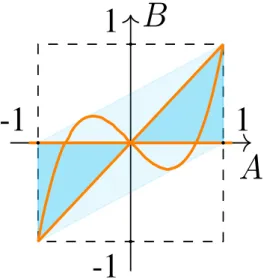
Fig. 2 shows whether a distribution can be modeled by an RNN (orange), an HMM (blue), a GUM (light blue) or none of them. For example, there is at least one instance of GUM modeling the distribution described by (A = 12, B =
1
distribution, some are actually HMM but none are RNN. In that example, the set of parameters (a = 13, b = 12, c = 13, η = 1) provides a proper solution (among others). As we see from the figure, any pdf in S can be obtained by at least one GUM; furthermore some can be produced by an HMM, but not by a RNN, and vice versa; finally some points can be reached by both.
Note that the expression of cov(Xt, Xt+τ) given in (12)
displays a behavior of the GUM already known in HMM and RNN; unless |a + bc| = 1, the current output is geometrically uncorrelated from the past outputs; in the case where |a+bc| = 1, (10) and (11) yield α = 0 and βc2 = 0. In other words,
to have long term dependencies, determinism through time is required. This phenomenon has already been observed in [4]. Let us now comment on the dimensionality of the models, which is related to the associated set of points in Figure 2. The RNN model is parameterized only by two parameters, η and the product bc (this product bc comes from the initialization constraint c2= η), whence the curve. By contrast the HMM
is parameterized by three parameters a, b and η, whence the two triangles.
A
B
-1
1
-1
1
Fig. 2: Modeling powers of RNN, HMM and GUM with regards to A and B. The parallelogram (light blue) coincides with all the multivariate centered Gaussian distributions with a covariance matrix which satisfy Cov(Xt, Xt+τ) = Aτ −1B.
Such distributions can be modeled by a GUM. The blue (resp. orange) areas (resp. curves) coincide with the value of A and B which can be taken by the HMM (resp. the RNN). This results shows that the modeling power of the GUM is larger than that of the HMM, which is larger than that of the RNN. However, let us note that in the context of this study, the RNN is finally defined by only 2 free parameters, the HMM relies on 3 parameters and the GUM on 4 parameters.
V. CONCLUDING REMARKS
In this paper we compared two popular models for pro-cessing time series, the HMM and the RNN. First, we have
encompassed both models in a common probabilistic model: both models can be seen as a particular instance of a GUM (whatever the activation function for the RNN, or the transition and likelihood distributions for the HMM). In order to address an exact comparison of the expressivity power of both models, we have focussed on the linear and Gaussian case. We have thus shown that the linear and Gaussian GUM can model a large class of stationary multivariate Gaussian distributions with geometrical covariance sequence. We also showed that none of the RNN or HMM sets is included into the other one, but that the modeling power of each model could easily be extended to the GUM framework, at the price of an augmentation of the number of parameters which characterize the model. However by considering deterministic transitions this price augmentation can be overcome. This highlights a more general trade-off between expressivity and practicability.
REFERENCES
[1] N. I. Akhiezer and N. Kemmer. The classical moment problem and some related questions in analysis, volume 5. Oliver & Boyd Edinburgh, 1965.
[2] M. Arulampalam, S. Maskell, N. Gordon, and T. Clapp. A tutorial on particle filters for online nonlinear / non-Gaussian Bayesian tracking. IEEE Transactions on Signal Processing, 50(2):174–188, February 2002. [3] D. Bahdanau, K. Cho, and Y. Bengio. Neural machine translation by
jointly learning to align and translate. ICLR, 2015.
[4] Y. Bengio and P. Frasconi. Diffusion of credit in markovian models. In Advances in Neural Information Processing Systems, pages 553–560, 1995.
[5] O. Cappé, É. Moulines, and T. Rydén. Inference in Hidden Markov Models. Springer Series in Statistics. Springer-Verlag, 2005.
[6] C.-C. Chiu, T. N. Sainath, Y. Wu, R. Prabhavalkar, P. Nguyen, Z. Chen, A. Kannan, R. J. Weiss, K. Rao, E. Gonina, et al. State-of-the-art speech recognition with sequence-to-sequence models. In 2018 IEEE International Conference on Acoustics, Speech and Signal Processing (ICASSP), pages 4774–4778. IEEE, 2018.
[7] J. Chung, C. Gulcehre, K. Cho, and Y. Bengio. Empirical evaluation of gated recurrent neural networks on sequence modeling. NeurIPS, 2014. [8] J. T. Connor, R. D. Martin, and L. E. Atlas. Recurrent neural networks and robust time series prediction. IEEE transactions on neural networks, 5(2):240–254, 1994.
[9] A. C. Harvey. Forecasting, structural time series models and the Kalman filter. Cambridge university press, 1990.
[10] J. J. Hopfield. Neural networks and physical systems with emergent collective computational abilities. Proceedings of the national academy of sciences, 79(8):2554–2558, 1982.
[11] R. Pascanu, T. Mikolov, and Y. Bengio. On the difficulty of training recurrent neural networks. In International conference on machine learning, pages 1310–1318, 2013.
[12] L. R. Rabiner. A tutorial on hidden Markov models and selected applications in speech recognition. Proceedings of the IEEE, 77(2):257– 286, 1989.
[13] B. Ristic, S. Arulampalam, and N. Gordon. Beyond the Kalman Filter: Particle Filters for Tracking Applications. Artec House, 2004. [14] R. H. Shumway and D. S. Stoffer. Time Series Analysis and Its
Applications (Springer Texts in Statistics). Springer-Verlag, Berlin, Heidelberg, 2005.