Identification of Robot Dynamic Parameters Using Jacobi Differentiator

HAL Id: hal-01164109

https://hal.archives-ouvertes.fr/hal-01164109

Submitted on 16 Jun 2015

HAL is a multi-disciplinary open access

archive for the deposit and dissemination of

sci-entific research documents, whether they are

pub-lished or not. The documents may come from

teaching and research institutions in France or

abroad, or from public or private research centers.

L’archive ouverte pluridisciplinaire HAL, est

destinée au dépôt et à la diffusion de documents

scientifiques de niveau recherche, publiés ou non,

émanant des établissements d’enseignement et de

recherche français ou étrangers, des laboratoires

publics ou privés.

Identification of Robot Dynamic Parameters Using

Jacobi Differentiator

Qi Guo, Maxime Gautier, Da-Yan Liu, Wilfrid Perruquetti

To cite this version:

Qi Guo, Maxime Gautier, Da-Yan Liu, Wilfrid Perruquetti. Identification of Robot Dynamic

Parame-ters Using Jacobi Differentiator. 2015 IEEE/ASME International Conference on Advanced Intelligent

Mechatronics (AIM), IEEE/ASME, Jul 2015, Busan, South Korea. �hal-01164109�

Identification of Robot Dynamic Parameters Using Jacobi Differentiator

Qi GUO

, Maxime GAUTIER

, Da-Yan LIU

and Wilfrid PERRUQUETTI

Abstract— This paper investigates the behavior of central Jacobi differentiator in robot identification applications. Jacobi differentiator is a Jacobi orthogonal based algebraic differen-tiator. It is applied to compute acceleration from noisy position measurements. Moreover, its frequency domain property is analyzed via a finite impulse response (FIR) filter point of view, indicating clearly the differentiators performance. In the end, a two revolute joints planar robot identification application is presented and comparisons between the Jacobi differentiator and the Euler differentiation combined with Butterworth filter are drawn.

I. INTRODUCTION

The topic on identification of robot dynamic parameters has been widely studied in the past decades, but there still exist several open questions. One of them is numerical dif-ferentiation, which concerns with estimating the derivatives of an unknown signal using its noisy measurement. This is an ill-posed problem in the sense that a small error in the measurement can produce a large error in the estimated derivatives, specially in the case of high order derivatives. Therefore, various numerical methods have been developed to obtain stable algorithms which are robust against corrupt-ing noises. They mainly fall into the followcorrupt-ing categories:

• finite difference methods [1],

• Savitzky Golay methods [2],

• wavelet differentiation methods [3],

• Fourier transform methods [4],

• mollification methods [5],

• Tikhonov regularization methods [6],

• algebraic methods [7], [8]

• differentiator observer [9], [10]

The recent algebraic differentiators are rooted in a recent algebraic parametric method introduced by Fliess and Sira-Ram´ırez [8], [11]. These algebraic differentiators are divided into two classes: model-based differentiators and model-free differentiators. The formers were obtained by applying the algebraic method to a differential equation which defines a class of linear systems [12], [13], [14]. Hence, they are mainly used for linear systems. However, the model-free 1_{Qi GUO, PhD student in CRIStAL (UMR CNRS 9189), ´Ecole Centrale}

de Lille, Villeneuve d’Ascq, 59650, France,qi.guo@ec-lille.fr

2_{Maxime GAUTIER, full professor in robotic group, Institut de}

Recherche en Communications et Cybern´etique de Nantes (IRCCyN), CNRS UMR 6597, ´Ecole Centrale de Nantes, Nantes, 44321, France,

Maxime.Gautier@irccyn.ec-nantes.fr

3 _{Da-Yan LIU, assistant professor in INSA Centre Val de Loire,}

Universit´e d’Orl´eans, PRISME EA 4229, Bourges Cedex 18020, France

dayan.liu@insa-cvl.fr

4_{Wilfrid PERRUQUETTI, full professor in Non-A INRIA-Lille Nord}

Europe & CRIStAL (UMR CNRS 9189) ´Ecole Centrale de Lille, Villeneuve d’Ascq, 59650, France,Wilfrid.Perruquetti@inria.fr

differentiators can be used for nonlinear systems. The first model-free differentiator was introduced in [15] by applying the algebraic method to the truncated Taylor series expansion of the signal to be differentiated. Then, two model-free differentiators were proposed in [16], where the causal Jacobi differentiator is presented. Moreover, it was shown that the causal Jacobi differentiator can also be obtained by taking the truncated Jacobi orthogonal series expansion of the signal to be differentiated. In [17], central Jacobi differentiator was proposed, which is devoted to off-line applications.

The algebraic differentiators have the following advan-tages. Firstly, they are given by exact integral formula. Thus, estimations at different instants can be obtained using a sliding integration window of finite length. Secondly, the integral formula can be considered as low-pass filters, which show robust properties with respect to corrupting noises [18]. The Jacobi differentiators contain some design parameters. Some error analysis has been done to study the influence of the design parameters [19], [20], [17], [21], where the study was based on some proposed error bounds. In this paper, the influence of the design parameters will be studied in a FIR filter point of view. For this purpose, their frequency domain properties are studied.

In order to identify robot dynamic parameters, a huge variety of methods have been proposed mainly using least-square techniques. The most widely applied approach is based on the robot explicit dynamic model, requiring joint acceleration data which are usually estimated from noisy measurement [22]. The other approaches are based on the robot energy model [23] or the robot power model [24], which require only joint velocity data, but instead they need a derivation operation on an implicit part of velocity. Besides, some authors utilize a parallel scheme to identify robot dynamic parameters by minimizing the output error from a closed loop simulation [25]. In this paper, the robot explicit dynamic model is considered under the condition that velocity and acceleration are well estimated using position data.

The paper is organized as follows: Section II introduces the robot dynamic model and discusses the identification process. Section III presents the central Jacobi differentiator and analyzes its frequency domain properties. Section IV obtains the identification results on a 2 joints planar direct drive prototype robot, respectively by means of the central Jacobi differentiator and the central Euler differentiation combined with the Butterworth filter. Finally, conclusions are given in Section V.

II. IDENTIFICATION

A. Explicit Dynamic Model

The explicit dynamic model of a rigid robot composed of

n moving links calculates the motor torque vector Γm as a

function of the state variables and their derivatives. It can be deduced from the following Lagrangian formulation:

Γm= d dt( ∂L ∂ ˙q)− ∂L ∂q+ Γf, (1)

where q, ˙q are the n×1 vectors of generalized joint position

and velocity, L is the Lagrangian of the system defined

as the difference between the kinetic energy E(q, ˙q) and

the potential energy U(q), with E = 1

2q˙

T_{M(q) ˙q, where} M(q) is the (n× n) robot inertia matrix. Γf is the friction

torque which is usually modelled at non zero velocity as:

Γfj = Fsjsign( ˙qj) + Fvj˙qj+ Γoffj, where ˙qj is the velocity

of joint j, sign(x) denotes the sign function. Fvj, Fsj are the

viscous and Coulomb friction coefficients of joint j, Γoffj

is an offset parameter which is the dis-symmetry of the Coulomb friction with respect to the sign of the velocity and is due to the current amplifier offset which supplies the motor [26] . Notice that the Coulomb friction contains

the non-linear term sign( ˙qj) which causes discontinuities on

Γf during the crossing of 0 velocity ˙qj. To avoid this, it is

replaced by a continuous 2_πarctan(αjq˙j) function, where αj

is a ratio of maximum joint velocity ˙qjmax

Develop Eq. (1) by replacing L with E− U, then it becomes

the explicit inverse dynamic model which depends on the joint acceleration:

Γm= M(q)¨q + C(q, ˙q) ˙q + Q(q) + Γf, (2)

where ¨q is the n× 1 vector of joint acceleration, M(q)

is the n× n symmetric and positive definite inertia matrix,

C(q, ˙q) ˙q is the n× 1 vector of Coriolis and centrifugal

torques, Q(q) is the n× 1 vector of gravity torques. The

dynamic model is linear with respect to a set of standard

dynamic parameters Xdyn. From (2) it can be rewritten as:

Γm= Ds(q, ˙q, ¨q)Xdyn. (3)

The vector Xdynis of dimension 14n×1, and for each link

there are 6 components of the inertia tensor, 3 components of the first moment, 1 mass parameter, 1 total inertia moment for rotor actuator and gears, 2 viscous and Coulomb friction parameters. According to [27], the set of standard dynamic parameters can be simplified into a set of base inertial parameters containing the minimum parameters that can describe the robot dynamics. They are obtained from the standard inertial dynamic parameters by eliminating those that have no effect on the dynamic model and by regrouping those in linear relations. In [28], symbolic and numerical solutions are presented for any open or closed chain robot manipulator to get a minimal dynamic model:

Γm= D(q, ˙q, ¨q)X, (4)

where X is the vector of base parameters.

B. Identification Process

Least squares (LS) technique is commonly used in robot dynamic parameters identification process by solving an

overdetermined linear system from ns sampling points of

the dynamic models (4) along a trajectory:

Y = W(q, ˙q, ¨q)X + ρ, (5) where ρ is a noise, Y and W are the vector of torques and the observation matrix, respectively, which are defined as follows: Y =    Γm(1) .. . Γm(ns)    , W =    D(1) .. . D(ns)    . (6)

The traditional method to estimate joint velocity ˙q and

acceleration ¨q is to apply central Euler difference of joint

position q. However, this method can amplify the noise effect

in the estimations of ˙q, ¨q. To avoid the noise distribution,

(q, ˙q, ¨q) must be filtered by a low-pass filter Fq(s), with

derivative operator s. The filter Fq(s) should have a flat

amplitude without phase shift in the range [0 ωcq], with

the rule of thumb ωcq > (10 × ωdyn), and ωdyn is the

bandwidth of the joint position closed loop [24]. Meanwhile,

the torque Γm is perturbed by high frequency torque ripple

from joint drive chain in the closed loop control. Hence, it

has to be filtered. Then, Γm and D(qfq, ˙qfq, ¨qfq) are both

filtered and downsampled through a decimate filter composed

of a low-pass filter Fp(s), where its cutoff frequency ωfp is

approximated by 5× ωdyn, in order to get a new filtered

linear system:

Yfp= Wfp(qfq, ˙qfq, ¨qfq)X + ρfp. (7)

Finally, we solve the LS problem via:

ˆ

X = W+_fp(qfq, ˙qfq, ¨qfq)Yfp, (8)

where W+_fp is the pseudo-inverse matrix of Wfp and ˆX is

the unique LS solution using the QR factorization or SVD

decomposition. ˆX minimizes the Euclidean norm∥ρ∥2of the

vector of errors ρ. The unicity of ˆX depends on the rank of

the observation matrix Wfp. The numerical rank deficiency

can come from Wfpstructural rank deficiency or

dissatisfac-tion of excitadissatisfac-tion condidissatisfac-tion due to a bad choice of samples. In order to decrease the sensitivity of LS solution with respect to errors, the condition number of the observation matrix must be close to 1. Some approaches used to calculate the exciting trajectory for identification are proposed in [29].

While in some cases the contribution of certain base parameters is too small that they cannot be experimentally identified even with optimized trajectories. Then, the base parameters should be replaced by a set of essential param-eters by eliminating certain insignificant paramparam-eters. There

are two approaches: the QR factorization of Wfpdiag( ˆX)

with column pivoting [30] or assuming that parameters with

relative standard deviation σ_Xˆ_j larger than 10% will be

essential parameters allows to improve the noise immunity of the robot identification process and reduce the computation burden for the model based control application.

III. CENTRALJACOBIDIFFERENTIATOR

Consider a noisy measurement xϖ _{: I → R, x}ϖ_{(t) =}

x(t) + ϖ(t), where I is a finite time open interval of R+,

x ∈ Cn(I) with n ∈ N, and ϖ is an additive corrupting

noise. The objective is to estimate the nth order derivative

of x using xϖ. First, for any t0 ∈ I, the set Dt0 =

{

t∈ R∗+; [t0− t, t0+ t]∈ I

}

is introduced.

A. Algebraic differentiator involving Jacobi polynomials

For any t0∈ I, x can be locally expressed on [t0−h, t0+

h] with h∈ Dt0 by the following Jacobi orthogonal series

expansion: ∀ ξ ∈ [−1, 1], x(t0+ hξ) = ∑ i≥0 ⟨ P_i(µ,κ)(·), x(t0+ h·) ⟩ µ,κ ∥P(µ,κ) i ∥2µ,κ P_i(µ,κ)(ξ), (9) where ⟨ P_i(µ,κ)(·), x(t0+ h·) ⟩ µ,κ= ∫1 −1wµ,κ(τ )P (µ,κ) i (τ )x(t0+ hτ )dτ , P (µ,κ) i is the ith order

Jacobi orthogonal polynomial defined on [−1, 1] as follows

(see [31]): P_i(µ,κ)(τ ) = i ∑ j=0 ( i + µ j )( i + κ i− j ) ( τ− 1 2 )i−j( τ + 1 2 )j , with µ, κ ∈] − 1, +∞[, ⟨·, ·⟩_µ,κ is a L2_{([−1, 1]) scalar}

product with the associated weight function wµ,κ(τ ) =

(1− τ)µ(1 + τ )κ, and the associated norm ∥P_i(µ,κ)∥2_µ,κ =

2µ+κ+1

2i+µ+κ+1

Γ(µ+i+1)Γ(κ+i+1)

Γ(µ+κ+i+1)Γ(i+1), where Γ(·) is the classical

Gamma function (see [31] p. 255).

In order to approximate x, the N + 1 first terms in the Jacobi series expansion given in (9) are taken, i.e. we locally

approximate x by a Nth_{order polynomial on [t}

0−h, t0+h].

Thus, by denoting the obtained Nth _{order polynomial by}

D_κ,µ,h,N(0) x(t0+ hξ), we have: ∀ ξ ∈ [−1, 1], D(0) κ,µ,h,Nx(t0+ hξ) := N ∑ i=0 ⟨ P_i(µ,κ)(·), x(t0+ h·) ⟩ µ,κ ∥P(µ,κ) i ∥2µ,κ P_i(µ,κ)(ξ). (10)

Hence, the value of x at t0 can be approximated by

D_κ,µ,h,N(0) x(t0) by taking ξ = 0. Inspired by this idea, the

central Jacobi differentiator is defined by taking the q + 1

(q = N− n ∈ N) first terms in the Jacobi series expansion

of x(n) _{with ξ = 0:} D_κ,µ,h,q(n) x(t0) = q ∑ i=0 ⟨ P_i(µ+n,κ+n)(·), x(n)_(t 0+ h·) ⟩ µ+n,κ+n ∥P(µ+n,κ+n) i ∥2µ+n,κ+n P_i(µ+n,κ+n)(0). (11)

This differentiator can be given by the following integral formula [17]: D_κ,µ,h,q(n) x(t0) = 1 hn ∫ 1 −1 Qκ,µ,n,q(τ ) x(t0+ hτ )dτ, (12) where ρn,κ,µ(τ ) =2 −(n+κ+µ+1)_{n!Γ(2n+κ+µ+2)} Γ(n+κ+1)Γ(n+µ+1) , Qκ,µ,n,q(τ ) = q ∑ i=0 P_iµ+n,κ+n(0) i ∑ j=0 (−1)i+j ( i j ) × 2i + κ + µ + 2n + 1 i + κ + µ + 2n + 1ρn,κ+i−j,µ+j(τ ).

Finally, x is substituted in (12) by xϖ in order to obtain

the Jacobi differentiator D(n)_κ,µ,h,qxϖ_(t

0) in noisy case.

It is clear that for each t0 ∈ I, the central Jacobi

differentiator D_{κ,µ,T ,q}(n) xϖ_(t

0) depends on a set of design

parameters, except for the order of the desired derivative n:

•κ, µ∈] − 1, +∞[: the parameters of Jacobi polynomials,

•q∈ N: the order of truncated Jacobi series expansion,

•T = 2h: the length of the sliding integration window. B. Error Analysis in Time Domain

The estimation error of the central Jacobi differentiator can be decomposed in continuous case as follows:

D(n)_κ,µ,h,qxϖ(t0)− x(n)(t0) = ( D(n)_κ,µ,h,qx− x(n)(t0) ) + ( D(n)_κ,µ,h,qxϖ(t0)− D (n) κ,µ,h,qx(t0) ) = eϖ(t0; n, κ, µ, h, q) + eRn(t0; κ, µ, h, q). (13)

where eϖ(t0; n, κ, µ, h, q) and eRn(t0; κ, µ, h, q) refer to the

noise error contribution and the truncated term error, respec-tively. Corresponding error bounds have been provided in

[17]. Finally, by numerically1_{calculating these error bounds,}

their behaviors with respect to different design parameters can be known. Then, the influence of these design parameters on each source of errors can be deduced. The obtained results are summarized in Table I (see [17], [32] for more details),

where the notations a ↑, b ↗ and c ↘ mean that if we

increase the value for the parameter a, then the error b can be increased and the error c can be decreased. According to Table I, the design parameters’ influence on different errors is not the same. Consequently, a compromise among these parameters should be taken.

Noise error contribution Truncated term error

κ↑ ↗ ↘

µ↑ ↗ ↘

q↑ ↗ ↘

T ↑ ↘ ↗

TABLE I: Influence of design parameters on D_κ,µ,h,q(n) x(t0)

in continuous case.

1_{It is very difficult to analytically study the behavior of each error bound}

In discrete case, the integral formula should be approx-imated by applying a numerical integration method, which produces a numerical error.

C. Error Analysis in Frequency Domain

As shown in Eq. (12), the Jacobi differentiator is a

com-bination of integrals with measurements on [t0−T₂, t0+T₂].

In real computation, the numerical integration is actually a

discrete operation, with a sampling time Tsin the

measure-ments by calculating the sum of discrete values in the time interval. The discrete version of the Jacobi differentiator is actually a discrete convolution of measurements and a list of weighted coefficients. In this sense, the Jacobi differentiator can be regarded as a FIR filter applied on a discrete system

with sampling time Ts. After extracting the weighted

coef-ficients, we can draw the bode magnitude plot of the Jacobi

differentiator, as a digital filter with sampling time Ts, in

order to express the magnitude of the frequency response. While in the bode phase plot, the phase frequency response

is always π or −π, which means that there is no delay.

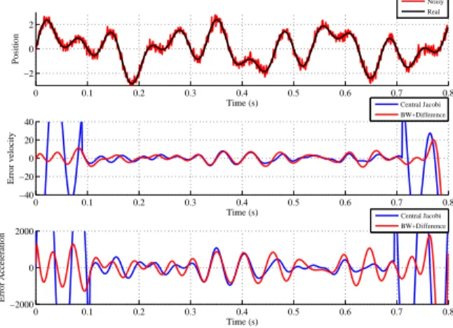
Given a signal that is the sum of three sinusoidal waves with amplitude 1 and frequency 4 Hz, 9 Hz, 15 Hz respec-tively. To get the second order derivative, the central Jacobi differentiator and the Euler central differentiation combined with a central Butterworth filter are applied. The central Butterworth filter is a zero phase forward-backward IIR filter and is referred as a maximally flat magnitude filter. It is widely used in various applications. Hence, this motivates the comparisons values.

The study is done in noise case, where the measurement of the signal is simulated by superimposing together on the signal a normally distributed random noise of amplitude 0.2, a 200 Hz high frequency sinusoidal wave of amplitude 0.2 and a Poisson distributed random noise with mean parameter

λ = 0.1 of amplitude 0.2. The sampling frequency is

1 millisecond. In order to estimate the derivatives of the original signal , the central Jacobi differentiator is applied by taking κ = µ = 12, q = 6 and the sliding integration window T = 0.21 second. A well tuned forward Butterworth filter configuration is of order 6 with cutoff frequency at 25 Hz. The forward-backward process is done by adding poles in the denominator of transfer function with negative values. The estimation errors in velocity and acceleration are shown in Fig. 1. The result shows that central Jacobi differentiator can be accurate and robust as Euler central differentiation with a well tuned Butterworth filter. It can be seen that the estimation errors for the central Jacobi differentiator is larger at the beginning and the end. This is because there is not enough data for the estimation.

In frequency domain, the magnitude bode plots of second order derivative are shown in Fig. 2. The red line presents the

ideal case with transfer function H(s) = s2 _{in continuous}

time. The Jacobi differentiator and Euler differentiation with Butterworth filter are in discrete case. Under 15 Hz, the magnitude frequency response follows quite well the ideal curve for both Jacobi differentiator and Butterworth method. Above 15 Hz, the magnitude frequency response cuts off

0 0.1 0.2 0.3 0.4 0.5 0.6 0.7 0.8 −2 0 2 Time (s) Position Noisy Real 0 0.1 0.2 0.3 0.4 0.5 0.6 0.7 0.8 −40 −20 0 20 40 Time (s) Error velocity Central Jacobi BW+Difference 0 0.1 0.2 0.3 0.4 0.5 0.6 0.7 0.8 −2000 0 2000 Time (s) Error Acceleration Central Jacobi BW+Difference

Fig. 1: Derivative errors in velocity and acceleration

Bode Diagram Frequency (Hz) 10−1 100 101 102 −250 −200 −150 −100 −50 0 50 100 150 200

System: Central Jacobi Frequency (Hz): 15 Magnitude (dB): 78.5 Magnitude (dB) Central Jacobi BW+Difference Real

Fig. 2: Bode magnitude plot of second order differentiators

rapidly especially for the Jacobi differentiator. This means that the Jacobi differentiator has a better cutoff property and the unexpected frequency is attenuated quickly to 0 magnitude response.

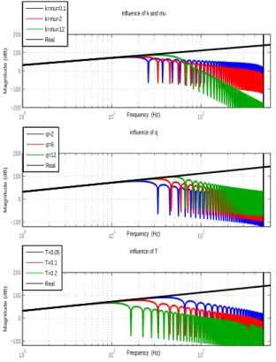
By varying the differentiator configuration, we can analyze the parameters’ influence on the central Jacobi differentiator. The obtained results are shown in Fig. 3, where the following conclusions are given:

1) κ = µ, these parameters are chosen to be identical because this configuration reduces the truncated term error [17]. As their value increases, the descending point moves to higher frequency. It means that the unwanted frequency is not filtered and the noise error contribution grows. But the descending period drops rapidly which offers better cutoff property.

2) When q increases, we utilize more terms in the Jacobi orthogonal series expansion. Hence, the truncated term error can be reduced. Similarly, as q increases, the descending point moves to higher frequency and the noise error contri-bution grows.

3) T is the sliding integration window. When the sampling

time Tsis fixed, it represents the points taken for the Jacobi

differentiator. As T increases, the descending point moves to lower frequency which cut off more noise components. Thus, the noise error contribution decreases.

100 101 102 −200 −100 0 100 200 Magnitude (dB) influence of k and mu Frequency (Hz) 100 101 102 −100 0 100 200 Magnitude (dB) influence of q Frequency (Hz) 100 101 102 −100 0 100 200 Magnitude (dB) influence of T Frequency (Hz) T=0.05 T=0.1 T=0.2 Real q=2 q=6 q=12 Real k=mu=0.1 k=mu=2 k=mu=12 Real

Fig. 3: Parameters influence on bode plot when Ts= 0.001s

From the previous analysis, the Jacobi differentiator is regarded as a low-pass differentiator. The low-pass property is inherent because it considers the signal as a certain order polynomial in a small time window and uses the truncations to estimate the derivatives. Compared to the Euler central differentiation combined with Butterworth filter, it can be more robust with respect to noise. However, it is used for off-line application, because the window in central

IV. EXPERIMENTALIDENTIFICATION WITH2R ROBOT

The experimental work is done on a two revolute joints planar prototype robot which is shown in Fig. 4. It moves in a horizontal plane and has no gravity effect. According to [33], the dynamic model depends on eight minimal base dynamic

parameters X = [ZZ1RZZ2MX2MY2FV1FC1 FV2FC2],

with the regrouped parameter ZZ1R= ZZ1+ M2L2, where

L is the length of first link, ZZ1 and ZZ2 are drive side

moment of inertial of link 1 and 2 respectively, MX2, MY2

are the first moment of link 2, FVj, FCj, are the viscous and

Coulomb friction coefficients of joint j.

The robot motion is driven by a PD controller with a reference of a successive point to point trajectories which

is obtained using a classical 5th_{order polynomial trajectory}

generator with a sampling rate fs= 100 Hz. For the central

Jacobi differentiator, set k = µ = 6, q = 2 and T = 0.6s to estimate the joint velocity, T = 1.1s to estimate the joint acceleration. For filtering method, the joint position and torque are pre-filtered using a fourth order forward-backward

Butterworth filter with a cutoff frequency fc= 0.1×(fs/2).

Fig. 4: 2R scara prototype robot

0 5 10 15 20 25 30 −4 −2 0 2 4 Time (s) Position 0 5 10 15 20 25 30 −2 0 2 Time (s) Velocity Central Jacobi Butterworth 0 5 10 15 20 25 30 −2 0 2 Time (s) Acceleration Central Jacobi Butterworth

Fig. 5: Real trajectory and estimation of velocities,

acceler-ation of q1

The estimations of velocity and acceleration are shown in Fig. 5.

The identification method is presented in section II. Then,

the estimation of base dynamic parameters ˆX is calculated

by LS method. Standard deviations σXˆi are estimated using

classical and simple results from statistics, assuming the matrix W to be a deterministic one, and ρ to be a zero mean

additive independent noise, with a standard deviation σρsuch

that Cρρ = E(ρTρ) = σ2ρIr, where E is the expectation

operator. The variance-covariance matrix of the estimation error and standard deviations can be calculated by:

C_{X ˆ}ˆ_X= E[( ˆX− ˆX)( ˆX− ˆX)T] = σ2ρ(W

T_W)−1_,

where σ2

ˆ

Xi

= C_{X ˆ}ˆ_Xii is the diagonal coefficient of C_{X ˆ}ˆ_X.

An unbiased estimation of σρ is used to get the relative

standard deviation σ_Xriˆ by the expression:

ˆ σ_ρ2= ||Y − W ˆX|| 2 r− c , %σXriˆ = 100× σXiˆ ˆ Xi,

where r is the total number of equations and c is the number of unknown parameters.

Identification results are given in table II which are quite similar for both methods. Compared to Butterworth filter

Jacobi Butterworth P Xˆ 2σ_Xˆ σ_Xrˆ Xˆ 2σ_Xˆ σ_Xrˆ % % ZZ1R 3.496 0.032 0.46 3.482 0.033 0.47 FV1 0.248 0.087 17.6 0.247 0.089 17.9 FC1 0.431 0.048 5.58 0.433 0.049 5.61 ZZ2 0.059 0.004 3.41 0.059 0.004 3.41 MX2 0.124 0.003 1.07 0.125 0.003 1.08 MY2 0.0019 0.002 65.99 0.0006 0.003 200 FV2 0.0144 0.015 52.3 0.014 0.015 54.4 FC2 0.1268 0.043 17.0 0.1272 0.043 17.1 number of equations= 522

cond(W ) = 38 for both cases

TABLE II: Comparison of experimental estimation

approach, the Jacobi differentiator method presents a better precision in identification results on error norm and relative error norm. When the trajectory is not of high frequency, the central Jacobi differentiator is a robust differentiator to get high order derivatives.

V. CONCLUSION

In this paper, the robot identification process has been reviewed by introducing the central Jacobi differentiator. By considering it as a FIR filter, its frequency domain properties have been investigated using bode plot and an insight into its differentiation performance has been given. Comparisons have been drawn between the Jacobi central differentia-tor and the Euler central differentiation combined with a well tuned forward-backward Butterworth filter. From the results, they all present good attenuation with respect to high frequency components. Especially, the Jacobi differentiator has a fast descending period, which make it resistant to high frequency noises. For future work, the causal Jacobi differentiator used for on-line applications will be studied.

REFERENCES

[1] I. Khan and R. Ohba, “New finite difference formulas for numerical differentiation,” J. Comput. Appl. Math., vol. 126, pp. 269–276, 2000. [2] A. Savitzky and M. Golay, “Smoothing and differentiation of data by simplified least squares procedures,” Anal. Chem., vol. 36, pp. 1627– 1638, 1964.

[3] X. Shao and C. Ma, “A general approach to derivative calculation using waveletnext term transform,” Chemometrics and Intelligent Laboratory

Systems, vol. 69, pp. 157–165, 2003.

[4] C. Fu, X. Feng, and Z. Qian, “Wavelets and high order numerical differentiation,” Appl. Math. Model., vol. 34, pp. 3008–3021, 2010. [5] D. H`ao, A. Schneider, and H. Reinhardt, “Regularization of a

non-characteristic cauchy problem for a parabolic equation,” Inverse Probl., vol. 11, no. 6, pp. 1247–1264, 1995.

[6] J. Cullum, “Numerical differentiation and regularization,” SIAM J.

Numer. Anal., vol. 8, pp. 254–265, 1971.

[7] C. Lanczos, Applied Analysis. Englewood Cliffs, NJ: Prentice-Hall, 1956.

[8] M. Fliess and H. Sira-Ramirez, “An algebraic framework for linear identification,” ESAIM controle optimisation et calcul des variations, vol. 9, p. 151, 2004.

[9] A. Levant, “Robust exact differentiation via sliding mode technique,”

Automatica, vol. 34, no. 3, pp. 379–384, 1998.

[10] A. Polyakov, D. Efimov, and W. Perruquetti, “Homogeneous differ-entiator design using implicit lyapunov function method,” in Control

Conference (ECC), 2014 European. IEEE, 2014, pp. 288–293.

[11] M. Fliess, M. Mboup, H. Mounier, and H. Sira-Ramirez, “Questioning some paradigms of signal processing via concrete examples,” in

Al-gebraic Methods in Flatness, Signal Processing and State Estimation.

Editorial Lagares, 2003, pp. pp–1.

[12] M. Fliess and H. Sira-Ramırez, “Reconstructeurs d’´etat,” Comptes

Rendus Mathematique, vol. 338, no. 1, pp. 91–96, 2004.

[13] Y. Tian, T. Floquet, and W. Perruquetti, “Fast state estimation in linear time-varying systems: an algebraic approach,” in Decision and

Control, 2008. CDC 2008. 47th IEEE Conference on. IEEE, 2008,

pp. 2539–2544.

[14] D.-Y. Liu, T.-M. Laleg-Kirati, W. Perruquetti, and O. Gibaru, “Non-asymptotic state estimation for a class of linear time-varying systems with unknown inputs,” in the 19th World Congress of the International

Federation of Automatic Control 2014, 2014.

[15] M. Fliess, C. Join, M. Mboup, and H. Sira-Ram´ırez, “Compression diff´erentielle de transitoires bruit´es,” Comptes Rendus Mathematique, vol. 339, no. 11, pp. 821–826, 2004.

[16] M. Mboup, C. Join, and M. Fliess, “A revised look at numerical differentiation with an application to nonlinear feedback control,” in

15th Mediterranean Conf. on Control and Automation (MED’07),

Athenes, Greece, 2007.

[17] D.-Y. Liu, O. Gibaru, and W. Perruquetti, “Differentiation by integra-tion with jacobi polynomials,” J. Comput. Appl. Math., vol. 235, pp. 3015–3032, 2011.

[18] M. Fliess, “Analyse non standard du bruit,” C.R. Acad. Sci. Paris Ser.

I, vol. 342, pp. 797–802, 2006.

[19] D.-Y. Liu, O. Gibaru, and W. Perruquetti, “Error analysis of jacobi derivative estimators for noisy signals,” Numerical Algorithms, vol. 50, no. 4, pp. 439–467, 2011.

[20] ——, “Convergence rate of the causal jacobi derivative estimator,” in

Curves and Surfaces. Springer, 2012, pp. 445–455.

[21] ——, “Synthesis on a class of algebraic differentiators and application to nonlinear observation,” in Control Conference (CCC), 2014 33rd

Chinese. IEEE, 2014, pp. 2592–2599.

[22] M. Gautier, “Identification of robots dynamics.” in IFAC/IFIP/IMACS

Symposium on Theory of Robots, 1986, pp. 125–130.

[23] M. Gautier and W. Khalil, “On the identification of the inertial parameters of robots,” in Decision and Control, 1988., Proceedings

of the 27th IEEE Conference on. IEEE, 1988, pp. 2264–2269.

[24] M. Gautier, “Dynamic identification of robots with power model,” in

Robotics and Automation, 1997. Proceedings., 1997 IEEE

Interna-tional Conference on, vol. 3. IEEE, 1997, pp. 1922–1927.

[25] M. Gautier, A. Janot, and P. O. Vandanjon, “Didim: A new method for the dynamic identification of robots from only torque data,” in Robotics

and Automation, 2008. ICRA 2008. IEEE International Conference on.

IEEE, 2008, pp. 2122–2127.

[26] M. Gautier, A. Janot, and P.-O. Vandanjon, “A new closed-loop output error method for parameter identification of robot dynamics,” Control

Systems Technology, IEEE Transactions on, vol. 21, no. 2, pp. 428–

444, 2013.

[27] H. Mayeda, K. Yoshida, and K. Osuka, “Base parameters of manipu-lator dynamic models,” Robotics and Automation, IEEE Transactions

on, vol. 6, no. 3, pp. 312–321, 1990.

[28] M. Gautier, “Numerical calculation of the base inertial parameters of robots,” Journal of Robotic Systems, vol. 8, no. 4, pp. 485–506, 1991. [29] J. Swevers, C. Ganseman, D. B. Tukel, J. De Schutter, and H. Van Brussel, “Optimal robot excitation and identification,” Robotics

and Automation, IEEE Transactions on, vol. 13, no. 5, pp. 730–740,

1997.

[30] P. Vandanjon and M. Gautier, “Reduction of robot base parameters,” CEA Centre d’Etudes de Saclay, 91-Gif-sur-Yvette (France). Dept. des Procedes et Systemes Avances, Tech. Rep., 1995.

[31] M. Abramowitz and I. Stegun, Eds., Handbook of mathematical

functions. GPO, 1965.

[32] D.-Y. Liu, “Error analysis of a class of derivative estimators for noisy signals and applications,” Ph.D. dissertation, Universit´e des Sciences et Technologie de Lille-Lille I, 2011.

[33] M. Gautier and W. Khalil, “Direct calculation of minimum set of inertial parameters of serial robots,” Robotics and Automation, IEEE