HAL Id: hal-01905469
https://hal.archives-ouvertes.fr/hal-01905469
Preprint submitted on 6 Nov 2018
HAL is a multi-disciplinary open access
archive for the deposit and dissemination of
sci-entific research documents, whether they are
pub-lished or not. The documents may come from
teaching and research institutions in France or
abroad, or from public or private research centers.
L’archive ouverte pluridisciplinaire HAL, est
destinée au dépôt et à la diffusion de documents
scientifiques de niveau recherche, publiés ou non,
émanant des établissements d’enseignement et de
recherche français ou étrangers, des laboratoires
publics ou privés.
Derivation of a polynomial equation for the boundaries
of 2-X manipulators
Matthieu Furet, Philippe Wenger
To cite this version:
Matthieu Furet, Philippe Wenger. Derivation of a polynomial equation for the boundaries of 2-X
manipulators. 2018. �hal-01905469�
boundaries of 2-X manipulators
Matthieu Furet and Philippe Wenger
Laboratoire des Sciences du Numérique de Nantes (LS2N), CNRS, Ecole Centrale de Nantes, 44321 Nantes, France
Abstract. This paper derives the boundary equations of the workspace of a manipulator made of two crossed four-bar mechanisms in series. The boundaries are determined with the discriminant of the characteristic polynomial derived for the inverse kinematics.
Keywords: Kinematics, crossed four-bar mechanism, anti-parallelogram, Workspace, Cuspidal
1
Introduction
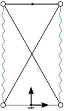
A crossed four-bar mechanism, referred to as X-mechanism, is a four-bar mech-anism assembled in a X-shape configuration, see figure 1. Because of a variable instantaneous center of rotation (ICR), this mechanism has a large range of motion. Moreover, tendon driven actuation can be easily implemented and a lightweight manipulator with remote actuation can be designed by stacking sev-eral such mechanisms [1]. Eventually, lateral springs can be added on each side of the mechanism, thus defining a X-shape Snelson tensegrity mechanism [2], suit-able for varisuit-able stiffness and natural interaction with the environment [3],[9]. This work is part of the AVINECK project involving biologists and roboticists with the main goal to model and design bird necks. Accordingly, a class of planar tensegrity manipulators made of a series assembly of several Snelson’s X-shape mechanisms has been chosen as a suitable candidate for a preliminary planar model of a bird neck. A planar two-degree-of-freedom manipulator is obtained with a series assembly of two such mechanisms. First investigations on the kine-matics of such manipulators have proven more challenging than expected, in particular for the solution of the inverse kinematics [10]. This paper derives the boundary equations of the workspace of a manipulator made of two crossed four-bar mechanisms in series. The boundaries are determined with the discriminant of the characteristic polynomial derived for the inverse kinematics. It is found that internal boundary curves may exist with cusp points [11], showing that the manipulator at hand is cuspidal ([15], [16]).
2
Manipulator modelling and Kinematic equations
The manipulators studied consist of a series assembly of two identical X-mecha-nisms as shown in figure 2. Both the base bar and the upper bar are of length
2 Matthieu Furet and Philippe Wenger
Fig. 1: Snelson’s X-shape mechanism made of a crossed four-bar mechanism with lateral springs
b and the two crossed links are of length L with L>b. Thus, each X-mechanism defines a so-called anti-parallelgramm joint. A line segment of length liis defined
that links the middle points of the top and base bars of each mechanism i (shown in red dotted line in figure 2). The angle between this line and the direction orthogonal to the base bar, referred to as θi, is used to define the configuration
of mechanism i without ambiguity, assuming that it remains always in its crossed-bar assembly mode [10]. Accordingly, the manipulator configuration can be fully defined with (θ1, θ2). To avoid any self collisions, the bars should be assembled
in different layers or suitable joint limits should be defined. The base frame is centered at the middle point of the base bar of the first X-mechanism with the x-axis aligned along this bar. The reference point (x, y) is chosen as the middle point of the top-bar of the second X-mechanism (figure 2). Since the sides of
θ1
θ2
l1
l2
(x,y)
Fig. 2: Manipulator description
each mechanism define an isosceles trapezoid, the length li of the line segment
that links the middle points of the top and base bars can be expressed as follows [10]:
li(θi) =
p
L2− b2cos2(θ
The direct kinematic equations of the 2-X manipulator can be put in the follow-ing form : ( x = −l1(θ1) sin(θ1) − l2(θ2) sin(2θ1+ θ2) y = l1(θ1) cos(θ1) + l2(θ2) cos(2θ1+ θ2) (2)
where l1 and l2 are defined in (1). Note that these equations assume that each
mechanism remains in its crossed-bar assembly-mode.
The inverse kinematics is much more challenging to establish and cannot be obtained from (2) easily. A methodology was proposed in [10], which makes it possible to derive a characteristic polynomial of degree four and it was shown that the manipulator may have up to four solutions.
3
Workspace boundary equations
The manipulator workspace is determined by means of its boundaries. These boundaries can be obtained from the discriminant of the 4th-order characteristic polynomial derived for the inverse kinematics. This characteristic polynomial in t=tan(φ1/2) was derived in [10] and is recalled below, where L has been set to
1 without loss of generality:
a4t4+ a3t3+ a2t2+ a1t + a0= 0 (3) where : a4= (b + 1)2(b2y2+ x4+ 2x2y2+ y4+ 4x3+ 4xy2+ 5x2+ y2+ 2x) (4) a3= 4y(b + 1)(2b2x + b2− 2x2− 2y2− 4x − 1) (5) a2= 2(b4y2+ b2x4+ 2b2x2y2+ b2y4+ b2x2− 10b2y2+ x4+ 2x2y2+ y4− 3x2+ 9y2) (6) a1= 4y(b − 1)(2b2x − b2+ 2x2+ 2y2− 4x + 1) (7) a0= (b − 1)2(b2y2+ x4+ 2x2y2+ y4− 4x3− 4xy2+ 5x2+ y2− 2x) (8)
The discriminant of this polynomial is derived with the help of a symbolic computing software. Accordingly, a polynomial equation of degree 16 in x and y is obtained as shown below.
4 b14y6+12 b12x4y4+28 b12x2y6+17 b12y8+12 b10x8y2+60 b10x6y4+112 b10x4y6+ 92 b10x2y8+28 b10y10+4 b8x12+36 b8x10y2+126 b8x8y4+224 b8x6y6+216 b8x4y8+ 108 b8x2y10+22 b8y12+4 b6x14+32 b6x12y2+108 b6x10y4+200 b6x8y6+220 b6x6y8+ 144 b6x4y10+ 52 b6x2y12+ 8 b6y14+ b4x16+ 8 b4x14y2+ 28 b4x12y4+ 56 b4x10y6+ 70 b4x8y8+ 56 b4x6y10+ 28 b4x4y12+ 8 b4x2y14+ b4y16− 24 b12x2y4− 36 b12y6− 48 b10x6y2 − 204 b10x4y4− 276 b10x2y6 − 120 b10y8 − 24 b8x10− 204 b8x8y2 − 612 b8x6y4−852 b8x4y6−564 b8x2y8−144 b8y10−36 b6x12−252 b6x10y2−720 b6x8y4− 1080 b6x6y6−900 b6x4y8−396 b6x2y10−72 b6y12−12 b4x14−84 b4x12y2−252 b4x10y4− 420 b4x8y6−420 b4x6y8−252 b4x4y10−84 b4x2y12−12 b4y14−8 b12y4+32 b10x4y2+
4 Matthieu Furet and Philippe Wenger 126 b10x2y4+102 b10y6+40 b8x8+332 b8x6y2+826 b8x4y4+816 b8x2y6+282 b8y8+ 110 b6x10+ 666 b6x8y2+ 1564 b6x6y4+ 1796 b6x4y6+ 1014 b6x2y8+ 226 b6y10+ 54 b4x12+ 324 b4x10y2+ 810 b4x8y4+ 1080 b4x6y6+ 810 b4x4y8+ 324 b4x2y10+ 54 b4y12− 4 b10x2y2+ 56 b10y4− 36 b8x6− 164 b8x4y2− 228 b8x2y4− 92 b8y6− 148 b6x8−716 b6x6y2−1244 b6x4y4−932 b6x2y6−256 b6y8−116 b4x10−572 b4x8y2− 1128 b4x6y4−1112 b4x4y6−548 b4x2y8−108 b4y10+4 b10y2+17 b8x4+14 b8x2y2− 143 b8y4+ 126 b6x6+ 294 b6x4y2+ 136 b6x2y4− 36 b6y6+ 141 b4x8+ 492 b4x6y2+ 622 b4x4y4+ 332 b4x2y6+ 61 b4y8+ 2 b2x10+ 6 b2x8y2+ 4 b2x6y4− 4 b2x4y6− 6 b2x2y8− 2 b2y10− 4 b8x2− 20 b8y2− 60 b6x4− 20 b6x2y2+ 172 b6y4− 132 b4x6− 200 b4x4y2+ 28 b4x2y4+ 96 b4y6− 16 b2x8− 32 b2x6y2+ 32 b2x2y6+ 16 b2y8+ 16 b6x2+40 b6y2+70 b4x4+16 b4x2y2−98 b4y4+38 b2x6+38 b2x4y2−38 b2x2y4− 38 b2y6− 24 b4x2− 40 b4y2− 28 b2x4− 8 b2x2y2+ 20 b2y4+ 16 b2x2+ 20 b2y2+ x4+ 2 y2x2+ y4− 4 x2− 4 y2= 0
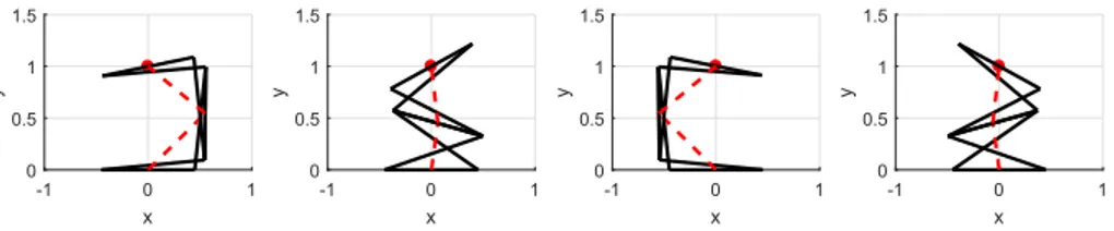
Figure 3 shows the plot of these boundary curves for three cases. In the second and third cases, they divide the workspace into three regions. In the largest one, the manipulator admits two inverse kinematic solutions. In the two smaller regions (filled in grey), there are four solutions. Figure4shows the four inverse kinematic solutions for the manipulator defined by L = 1 and b = 9/10, at x = 0, y = 1. -2 -1 0 1 2 x -2 -1 0 1 2 y -2 -1 0 1 2 x -2 -1 0 1 2 y -2 -1 0 1 2 x -2 -1 0 1 2 y
Fig. 3: Workspace boundaries when L = 1 and b = 2/5 (left), b = 2/3 (center), b = 9/10 (right) -1 0 1 x 0 0.5 1 1.5 y -1 0 1 x 0 0.5 1 1.5 y -1 0 1 x 0 0.5 1 1.5 y -1 0 1 x 0 0.5 1 1.5 y
4
Conclusion
The equation of the boundary curves of the workspace of a 2-X manipulator was derived using the discriminant of the characteristic polynomial derived for the inverse kinematics. The resulting polynomial is of degree 16 and, under some geometric conditions, reveals regions with four inverse kinematic solutions. Moreover, the boundary curves of the 4-solution regions feature two cusp points and one node.
Acknowledgement This work has been conducted in part with the support of the French National Research Agency (AVINECK Project ANR-16-CE33-0025).
References
1. K. Moored et al., Analytical predictions, optimization, and design of a tensegrity-based artificial pectoral fin, Int. J. of Solids and Structures, Vol. 48, pp3142-3159, 2011
2. K. Snelson, Continuous Tension, Discontinuous Compression Structures, US Patent No. 3,169,611, 1965
3. D. L Bakker et al., Design of an environmentally interactive continuum manipula-tor, Proc.14th World Congress in Mechanism and Machine Science, IFToMM’2015, Taipei, Taiwan, 2015
4. R. B. Fuller, Tensile-integrity structures, United States Patent 3063521,1962 5. Skelton, R. and de Oliveira, M., Tensegrity Systems. Springer, 2009
6. S. Levin, The tensegrity-truss as a model for spinal mechanics: biotensegrity, J. of Mechanics in Medicine and Biology, Vol. 2(3), 2002
7. M. Arsenault and C. M. Gosselin, Kinematic, static and dynamic analysis of a planar 2-dof tensegrity mechanism, Mech. and Mach. Theory, Vol. 41(9), 1072-1089, 2006 8. C. Crane et al., Kinematic analysis of a planar tensegrity mechanism with
pres-stressed springs, in Advances in Robot Kinematics: analysis and design, pp 419-427, J. Lenarcic and P. Wenger (Eds), Springer (2008)
9. P. Wenger and D. Chablat, Kinetostatic Analysis and Solution Classification of a Planar Tensegrity Mechanism, proc. 7th. Int. Workshop on Comp. Kinematics, Springer, ISBN 978-3-319-60867-9, pp422-431, 2017.
10. M. Furet et al., Kinematic analysis of planar 2-X tensegrity manipulators, Proc. Advances in Robot Kinematics, Bologna, Italy, June 2018.
11. M. Furet and P. Wenger, Workspace and cuspidality analysis of a 2-X planar manipulator, Proc. 4th IFToMM Symposium on Mechanism Design for Robotics, Udine, Italie, 2018.
12. Q. Boehler et al., Definition and computation of tensegrity mechanism workspace, ASME J. of Mechanisms and Robotics, Vol 7(4), 2015
13. JB Aldrich and RE Skelton, Tienergy optimal control of hyper-actuated me-chanical systems with geometric path constraints, in 44th IEEE Conference on De-cision and Control, pp 8246-8253, 2005
14. S. Chen and M. Arsenault, Analytical Computation of the Actuator and Cartesian Workspace Boundaries for a Planar 2-Degree-of-Freedom Translational Tensegrity Mechanism, Journal of Mech. and Rob., Vol. 4, 2012
15. J. El Omri and P. Wenger, How to recognize simply a non-singular posture changing manipulator, Proc. 7th Int. Conf. on Advanced Robotics, 215-222, 1995
6 Matthieu Furet and Philippe Wenger
16. P. Wenger, Cuspidal and noncuspidal robot manipulators. Special issue of Robotica on Geometry in Robotics and Sensing, Volume 25(6), pp.677-690, 2007
17. F. Thomas and P. Wenger, , On the Topological Characterization of Robot Singu-larity Loci. A Catastrophe-Theoretic Approach, IEEE International Conference on Robotics and Automation ICRA 2011, 9-13 mai 2011, Shanghai.
18. P. Wenger, D. Chablat, M. Baili, A DH parameter based condition for 3R orthog-onal manipulators to have four distinct inverse kinematic solutions, ASME Journal of Mechanical design, Vol. 127(1), pp 150-155, 2005