Factor Analysis of a Large DSGE Model

Factor Analysis of a Large DSGE Model

Alexei Onatski Francisco J. Ruge-Murciay September 27, 2010

Abstract

We study the workings of the factor analysis of high-dimensional data using arti…cial series generated from a large, multi-sector dynamic stochastic general equilibrium (DSGE) model. The objective is to use the DSGE model as a laboratory that allow us to shed some light on the practical bene…ts and limitations of using factor analysis techniques on economic data. We explain in what sense the arti…cial data can be thought of having a factor structure, study the theoretical and …nite sample properties of the principal components estimates of the factor space, investigate the substantive reason(s) for the good performance of di¤usion index forecasts, and assess the quality of the factor analysis of highly dissagregated data. In all our exercises, we explain the precise relationship between the factors and the basic macroeconomic shocks postulated by the model.

JEL Classi…cation: C3, C5, E3

Keywords:Multisector economies, principal components, forecasting, pervasiveness, FAVAR.

Faculty of Economics, University of Cambridge, Sidgwick Avenue, Cambridge, CB3 9DD, United Kingdom. E-mail: ao319@econ.cam.ac.uk

y_{Département de sciences économiques and CIREQ, Université de Montréal, C.P. 6128, succursale Centre-ville,}

1.

Introduction

Large factor models have been playing an increasingly important role in empirical macroeconomic research. Their use is often motivated by the fact that modern dynamic general equilibrium models postulate the existence of only a few common sources of ‡uctuations for all macroeconomic vari-ables. Much of the research takes this fact a step further and identi…es the factor space with the space of basic macroeconomic shocks. This interpretation is then exploited to carry out structural factor analysis.1 Although the statistical workings of large factor models and of their forecast-ing and structural applications are well understood by now, their macroeconomic content remains largely unexplored. Usually, the existence of such a macroeconomic content is simply a matter of assumption or believe. In particular, the relationship between the factor space and the space of macroeconomic shocks has never been analyzed in the context of a theoretical macroeconomic model. The reason is that few general equilibrium models describe the dynamics of a large enough number of disaggregated macroeconomic series to provide the basis for a substantive analysis of large factor models.

This paper studies the workings of the factor analysis of high-dimensional data using arti…cial series generated from a dynamic stochastic general equilibrium (DSGE) model. The intention is to use the fully-speci…ed DSGE model as a laboratory to understand the practical bene…ts and limitations of using factor analysis techniques on economic data. We pursue this approach because in contrast to actual economic data, whose generating process is unknown, the arti…cial data from a model comes from a process that is known and under the control of the econometrician. As DSGE model we use the highly disaggregated multi-sector model developed and estimated by Bouakez, Cardia and Ruge-Murcia (2009). Several features of this model make it particularly suitable for our analysis. First, it speci…es thirty heterogenous productive sectors that correspond to the two-digit level of the Standard Industrial Classi…cation (SIC) and so it can generate a large number of disaggregated series to which one can meaningfully apply factor analysis techniques. Second, the model features aggregate shocks but also sector-speci…c shocks which may be transmitted to other sectors through the input-output structure of the economy. Thus, as in the actual data, the notion of what “factors” are is not trivial. Finally, although the model is (by de…nition) a stylized representation of the economy, it is rich enough to shed some light on the application of factor analysis to actual disaggregated data.

In this project, we explain in what sense the data generated from the model can be thought of as having a factor structure, study the theoretical and …nite sample properties of the principal

1

components estimates of the factor space, investigate the performance of di¤usion index forecasts, and assess the quality of the factor analysis of highly dissagregated data. In all our exercises, we explain the precise relationship between the factors and the basic macroeconomic shocks postulated by the model.

We …nd that the three economy-wide shocks of Bouakez et al. (2009), namely the monetary policy shock, the money demand shock and the leisure preference shock, can indeed be thought of as factors because they non-trivially a¤ect most of the 156 variables generated by the model. Moreover, the remaining 30 sectoral productivity shocks signi…cantly a¤ect only a small number of the variables. However, despite the pervasiveness of the economy-wide shocks, the principal components analysis has a hard time replicating the macroeconomic factor space. We document and explain the di¢ culties that arise and assess the quality of the asymptotic approximation to the distribution of the principal components, …nd it unsatisfactory, and analyze the reasons for such a failure.

Further, we show that the di¤usion index forecasts of output growth and of aggregate in‡ation perform reasonably well on our simulated data. In particular, accurately estimating the macroeco-nomic factor space turns out to be not essential for the quality of the forecasts of our data. We decompose the di¤usion index forecast error into several components and study them in detail.

Finally, we use our data to investigate the workings of the factor augmented vector autore-gression (FAVAR) analysis of disaggregated data. We are especially interested in the question of whether the monetary policy impulse responses of the disaggregated series estimated by a FAVAR …tted to our data accurately recover the true impulse responses. Somewhat surprisingly, we …nd that the quality of the estimated impulse responses of the sectoral variables is very good.

The rest of the paper is organized as follows. Section 2, describes the data generating process. (A very detailed description of the DSGE model and parameter values used to generate the arti…cial data is also given in the Appendix.) Section 3 explains in what sense our data has a dynamic factor structure and studies the relationship between the space of dynamic factors, represented by the economy-wide shocks, and the space of dynamic principal components. Section 4 compares the spaces spanned by the lags of the dynamic factors and by the population static and generalized principal components. Section 5 studies the determination of the number of factors. Section 6 compares the population and sample principal components. Section 7, analyzes the di¤usion index forecasts. Section 8 performs a FAVAR analysis of the monetary policy e¤ects on the disaggregated variables. Finally, Section 9 concludes.

2.

Data generating process

The data generating process (DGP) is based on the large multi-sector DSGE model in Bouakez, Cardia and Ruge-Murcia (2009) (BCR in what follows). Their model features thirty sectors or industries that roughly correspond to the two-digit level of the Standard Industrial Classi…cation (SIC). Sectors are heterogenous in production functions, price rigidity, and the combination of materials and investment inputs used to produce their output. The productive structure is of the roundabout form, meaning that each sector uses output from all sectors as inputs, although in a manner consistent with the actual U.S. Input-Output and Capital-Flow Tables. In addition, sectors are subject to idiosyncratic productivity shocks. There is a representative consumer who supplies labor to all sectors, and derives utility from leisure, real money balances, and the consumption of goods produced by all sectors.

Economic ‡uctuations arise from three aggregate (or economy-wide) shocks and thirty sectoral shocks. The aggregate shocks are shocks to the representative consumer’s utility from leisure and from holding real money balances, and a monetary policy shock, which is modeled as a shock to the growth rate of the money supply. The thirty productivity shocks are sector-speci…c in that they originally disturb only the production function of their own sector. However, as a result of input-output interactions between sectors, idiosyncratic productivity shocks are transmitted to other sectors and to economic aggregates. All the thirty-three shocks of the model are assumed to follow independent univariate AR(1) processes. The model is described in more detail in the Appendix. The values of the model parameters are those estimated by Bouakez, Cardia and Ruge-Murcia (2009) using quarterly aggregate and sectoral U.S. data from 1964:Q2 to 2002:Q4 and are listed in the Appendix as well.

We solve the log-linearized equations of the BCR model using the standard Blanchard and Khan (1980) algorithm. Collecting the log-linear approximations to the equilibrium decision rules and arranging them into the state-space form, we can write the state-space representation of the data generating process:

Xt+1 = AXt+ B"t (1)

Yt = CXt+ D"t:

The meaning of the variables "t; Ytand Xtis as follows. The 33-dimensional vector "tconsists of

the 30 unit-variance innovations to the sector-speci…c productivity shocks and three unit variance innovations to the economy-wide shocks, namely the leisure preference shock, the money demand shock and the monetary policy shock. The 156-dimensional vector of simulated data Yt consists of

stacked 1 30 vectors of the percentage deviations from the steady state of the sectoral outputs, sec-toral hours worked, secsec-toral wages, secsec-toral consumptions, and secsec-toral in‡ations; scalar aggregate output, hours worked, wages, consumption, and in‡ation; and scalar rates of money growth and nominal interest. The state vector Xt is a linear combination of sectoral and aggregate variables.

The choice of the state vector is not unique and it is usually made so that the dimension of the matrix A is as small as possible. In our case, the smallest possible dimension is 101.2

For the numerical values of A; B; C and D in (1), we check that the innovations "t can be

recovered from the history of Yt; and thus, they are fundamental. Fernandez-Villaverde et al.

(2007) describe a simple criterion for checking the fundamentalness of innovations when D is a square invertible matrix. In our case, D is 156 33 so that the criterion cannot be directly applied. However, we can use the criterion for checking the fundamentalness of "tin the system

Xt+1 = AXt+ B"t

~

Yt = CX~ t+ ~D"t;

where ~Yt= R0Yt; ~C = R0C, ~D = R0D and R is any 156 33 matrix. We choose R so that it consists

of the …rst 33 columns of matrix U from the singular value decomposition of D : D = U SV:3 Then, we form the matrix M = A B ~D 1C and check numerically that all its eigenvalues are less than~ one in absolute value, which, according to Fernandez-Villaverde et al. (2007), insures that "t can

be recovered from the history of ~Yt R0Yt; and therefore, from the history of Ytitself.

Equations (1) can be used to express the simulated data as an in…nite lag polynomial of the innovations "t:

Yt=

h

CL (I AL) 1B + Di"t A(L)"t; (2)

where L is the lag operator. The i; j-th entry of the matrix coe¢ cient on the p-th power of L in the polynomial A(L) equals the impulse response of the i-th variable in the data to a one-period unit impulse in the j-th component of the innovation vector "t:

3.

The dynamic factor structure and principal components

Let ftbe the three-dimensional vector of economy-wide shocks. As was mentioned before, they are

modeled as independent AR(1) processes so that

ft= ft 1+ f"f t; 2

We used MATLAB’s Control System toolbox command minreal to obtain the minimal state-space realization in (1), which turned out to have a state vector of dimensionality 101.

3_{Such a choice maximizes the smallest eigenvalue of ~D ~D}0 _{= R}0_DD0_{R among all R with kRk = 1; where kRk}

where "f t are the standardized innovations to the economy-wide shocks, f are scaling parameters,

and is a 3 3 matrix with the autoregressive coe¢ cients along the main diagonal and zero everywhere else. We can decompose the MA(1) representation of the model (2) into a part that depends on ft j with j = 0; 1; :::; and the orthogonal part:

Yt= (L) ft+ et; (3)

where (L) = Af(L) f1(I3 L) with I3 the 3 3 identity matrix, et = Ae(L) "et; "et is the

vector of the innovations to the sector-speci…c shocks, and Af(L) and Ae(L) are the parts of A(L)

corresponding to the economy-wide and sector-speci…c shocks, respectively.

In what follows, we will always standardize Yt so that the variance of each of its components

equals unity. It is convenient to introduce new notation for such a standardized Yt: Let W be

the inverse of the diagonal matrix with the standard deviations of the components of Yt on the

diagonal: Then, the standardized version of Yt equals Yt(s) = W Yt; and it admits the following

decomposition

Y_t(s)= (s)(L) ft+ e (s) t ;

where (s)(L) = W (L) and e(s)_t = W et:

Intuitively, we would call (3) a factor decomposition if the “factors” ft had a pervasive e¤ect

on the elements of Yt whereas the “idiosyncratic” terms eit did not have pervasive e¤ects on the

elements of Yt: Such requirements are in the spirit of all high-dimensional factor models starting

from the approximate factor model of Chamberlain and Rothschild (1983). We will now examine how pervasive ft and "et are in our arti…cial data.

3.1 Pervasiveness

An intuitive measure of the pervasiveness of a given shock in a particular dataset can be obtained as follows. For each variable in the dataset, compute the percentage of the variance of this variable due to the given shock. Then, compute and plot the percentage y(z) of the variables in the dataset for which the shock explains at least z% of the variance. Note that such a measure of pervasiveness does not depend on whether we analyze Yt or its standardized version Yt(s): Pervasive shocks

non-trivially a¤ect a large number of the variables in the dataset. Therefore, for such shocks, y(z) should decrease slowly in z: In contrast, for non-pervasive shocks, we expect y(z) to be dramatically decreasing to zero as z becomes slightly larger than zero.

Figure 1 shows the pervasiveness measures y(z) for all the 33 shocks of the BCR model. As one would intuitively expect, the economy-wide shocks ft stand out as much more pervasive than the

0 20 40 60 80 100 0 10 20 30 40 50 60 70 80 90 100

Percentage of the variance explained

Per c en tag e of t he v ar iabl es

Pervasiveness of different innovations

Leisure preference

Monetary policy

Money demand

Figure 1: Pervasiveness of di¤erent shocks in BCR model.

30% of variance for about 2/3 of all the variables in our dataset. The monetary policy shock is also pervasive, explaining 30% of the variance for more than 40% of the variables. The money demand shock is the least pervasive of the three. Even so, it explains more than 10% of the variance for more than 25% of the variables. The next most pervasive shock is the productivity shock in the agricultural sector: It explains more than 10% of the variance for only about 3.8% of variables.

We can extend our measure of pervasiveness to a frequency-by-frequency measure. In principle, we can de…ne a measure of pervasiveness y(z; !) for "j as the percentage of the components of Y

for which the percentage of the variance at frequency ! explained by "j is less than z: However, it

would be di¢ cult to report such a pervasiveness measure for the 33 shocks on the same plot. We, therefore, restrict our attention to a pervasiveness measure corresponding to three frequency bands: low frequencies, business cycle frequencies and high frequencies. We de…ne the low frequency band as the set of all frequencies which correspond to cycles of more than 8 years per period, the business cycle frequencies as those corresponding to cycles in between 2 and 8 years per period, and the high frequencies as those corresponding to cycles of less than 2 years per period.

We de…ne yLF_{j (z) as the percentage of such i 2 fi = 1; 2; :::; 156g for which} Z !2LF jA ij(!)j2d! z 100 33 X j=1 Z !2LF jA ij(!)j2d!;

0 20 40 60 80 100 0 50 100 Low f requenc es 0 20 40 60 80 100 0 50 100 B u si n e ss cycl e 0 20 40 60 80 100 0 50 100 H igh fr equenc es Leisure preference Monetary policy Monetary policy Leisure preference Money demand Monetary policy Money demand Leisure preference

Figure 2: Frequency-by-frequency pervasiveness of di¤erent shocks in the BCR model.

variables for which shock j is responsible for at least z% of the variance at low frequencies. We similarly de…ne y_jBF(z) and yHF_j (z) for business cycle and high frequencies.

Figure 2 shows plots of y_jLF(z) (upper panel), y_jBF(z) (middle panel) and y_jHF(z) (lower panel). We see that for low frequencies only two shocks are pervasive: the leisure preference shock and the monetary policy shock. For business cycle frequencies all three economy-wide shocks are pervasive. However, the leisure preference shock is considerably less pervasive than the money demand shock and, especially, than the monetary policy shock. For high frequencies, the pervasiveness of the leisure preference shock almost completely disappears, whereas the monetary policy and money demand remain pervasive.

Hence, for our data, di¤erent frequencies correspond to di¤erent shocks being pervasive. More-over, the number of the pervasive shocks varies from frequency to frequency. This observation suggests that, from the empirical perspective, it may be desirable to relax the assumption of the generalized dynamic factor models that the number of the exploding eigenvalues of the spectral density matrix of the data remains the same for all frequencies.

3.2 Heterogeneity

The pervasiveness of the economy-wide shocks is a necessary but not su¢ cient condition for success-ful recovery of the space spanned by all lags and leads of such shocks by the principal components

analysis. For such a recovery, the economy-wide shocks must generate heterogeneous enough re-sponses from the observed variables. The reason is that the model Y_t(s) = (s)(L) ft + e(s)t is

equivalent to Y_t(s) = ~(s)(L) ~ft+ e (s)

t ; where ~(s)(L) = (s)(L) U (L); ~ft = U (L 1)0ft and U (L)

is a so-called Blaschke matrix (see Lippi and Reichlin, 1994), that is a matrix of polynomials in L such that det U (z) 6= 0 for z on the unit circle and U (z) U(z 1)0 = I; where the bar over a polynomial matrix denotes the polynomial matrix with complex conjugated coe¢ cients. Therefore, for the successful recovery, not only ft; but also ~ft must be pervasive. If the columns of (L)

are not heterogeneous enough so that some of their linear combinations with coe¢ cients that are polynomials in L is small (in terms of the sum of squares of all the coe¢ cients on the di¤erent powers of L), then one can choose U (L) so that at least one component of ~ft is not pervasive, and

therefore, the principal components analysis will not accurately recover the space spanned by all lags and leads of ~ft; and hence of ft.

Furthermore, for successful recovery of the space spanned by all lags and leads of the economy-wide shocks by the principal components analysis, the responses from the observed variables to the sector-speci…c shocks must be heterogeneous enough. Indeed, if such a responses were similar, then there would exist a linear combination of the sector-speci…c shocks that generate a particularly large response from the observed variables. The variance of the data explained by such a linear combination would be large, and therefore, it could be confused for a genuine factor by the principal components analysis.

A convenient tool for the joint analysis of pervasiveness and heterogeneity is the eigenvalues of the spectral density matrices of the factor and idiosyncratic components of the data. Such eigenvalues are invariant with respect to the di¤erent choices of Blaschke matrices U (L) in the above equations. Let Sf(!) be the spectral density matrix of (s)(L) ft: The largest eigenvalue of

Sf(!) measures the maximum amount of the variation of the (standardized) data at frequency !

explained by a white-noise shock ~f1t that belongs to the space spanned by the lags and leads of the

economy-wide shocks. The second largest eigenvalue of Sf(!) measures the maximum amount of

the variation of the data at frequency ! explained by a white-noise shock ~f2t which is orthogonal

to ~f1t at all lags and leads and which belongs to the space spanned by the lags and leads of the

economy-wide shocks. The third largest eigenvalue of Sf(!) is the last non-zero eigenvalue of

Sf(!) because there are only three economy-wide shocks in our model. This eigenvalue measures

the minimum amount of the variation of the data at frequency ! explained by a white-noise shock ~

f3t that belongs to the space spanned by the lags and leads of the economy-wide shocks. The three

non-zero eigenvalues of Sf(!) can be viewed as one-dimensional summaries of the pervasiveness of

10-2 10-1 100 10-2 10-1 100 101 102 103 104 Frequencies E ig env alu es

Figure 3: The three largest eigenvalues of Sf(!) (solid lines), the largest eigenvalue of Se(!) (dashed

line), and the largest eigenvalues of Sf 1(!); Sf 2(!) and Sf 3(!) (dotted lines):

Sf(!) is relatively small uniformly over ! 2 [0; 2 ); then the responses from the observed variables

to the economy-shocks ftmust be not heterogeneous. We would hope that the principal components

analysis accurately recovers the space spanned by all lags and leads of the economy-wide shocks only if the third largest eigenvalue of Sf(!) is larger than the largest eigenvalue of the spectral

density matrix Se(!) of the idiosyncratic component e(s)t uniformly over ! 2 [0; 2 ):

Figure 3 shows that only the largest eigenvalue of Sf(!) is uniformly larger than the largest

eigenvalue of Se(!) over ! 2 [0; 2 ):4 The second largest eigenvalue of Sf(!) is smaller than the

largest eigenvalue of Se(!) for relatively high frequencies ! > 1; which correspond to ‡uctuations

with periods smaller than 2 quarters. The third largest eigenvalue of Sf(!) is uniformly smaller

than the largest eigenvalue of Se(!) over ! 2 [0; 2 ): Hence, we expect (an imperfect) recovery of

at most two orthogonal linear …lters of the three-dimensional factor ftby the principal components

analysis.

The dotted lines on Figure 4 show the largest eigenvalues of the spectral densities Sf 1(!) ;

Sf 2(!) and Sf 3(!) of the components of the observables that correspond to the monetary policy

shock, to the money demand shock and to the leisure preference shock, respectively. These eigen-4_{The horizontal and the vertical scales of the graph are made logarithmic to enhance visibility.}

values are all larger than the largest eigenvalue of Se(!) at frequencies ! > 0:1; which correspond to

‡uctuations with periods smaller than 20 quarters, including business cycles, which typically are thought as having periods no larger than 8 or 10 years. Nevertheless, we expect that the business cycle components of the economy-wide shocks cannot be recovered by the principal components analysis. The reason is that the e¤ects of the economy-wide shocks on the observables are not heterogeneous enough, which is re‡ected in the fact that the third largest eigenvalue of Sf(!) is

substantially smaller than the minimum of the largest eigenvalues of Sf 1(!) ; Sf 2(!) and Sf 3(!)

for all ! 2 [0; 2 ):

We checked that the largest eigenvalue of Se(!) is very close to the maximum of the largest

eigenvalues of the spectral densities Sei(!) ; i = 1; :::; 30 of the thirty components of the data

corresponding to the sector-speci…c shocks. Therefore, the potential problem with the principal components analysis is indeed caused by the similarity in the e¤ects of the economy-wide shocks and not by a possibility that a particular linear …lter of the sector-speci…c shocks have an unusually strong e¤ect on the observables. Similarly, in actual economies di¤erent aggregate shocks may also generate similar dynamics on (a subset of) observable variables. For example, in a money-growth targeting regime, changes in monetary aggregates would have similar e¤ects on, say, output variables, regardless of whether they are the result of changes in the monetary base by the central bank or in lending behavior by commercial banks.

3.3 The content of the dynamic principal components

Estimation of the pervasive factors and the factor loadings in large factor models is often based on the sample principal components analysis. In this subsection, we perform the population principal components analysis to determine the theoretical limit to the principal-component-based extraction of the pervasive shocks for our standardized data.

As mentioned above, we expect (an imperfect) recovery of at most two orthogonal linear …lters of the three-dimensional factor ft because the dynamic e¤ects of the economy-wide shocks on the

observables are not heterogeneous enough. Speci…cally, we expect the …rst two dynamic principal components to be close to some …lters of ft; and the third dynamic principal component to have a

very large sector-speci…c part. We now check this conjecture.

Recall that the dynamic principal components of Y_t(s) are de…ned as follows.5 Let SY (!) be

the spectral density matrix of the standardized data and let j(!) and pj(!) be its j-th largest

eigenvalue and the corresponding unit-length row eigenvector, respectively, so that pj(!) SY (!) = j(!) pj(!). Consider the Fourier expansion for pj(!) : pj(!) = (1=2 )P1_{k= 1}Pjke ik!; where

Pjk =

R

pj(!) eik!d!: Let pj(L) equal (1=2 )P1_{k= 1}PjkLk: Then, the j-th dynamic principal

component of Y_t(s) is de…ned as jt pj(L) Yt(s). Or, in terms of the innovations to the economic

shocks:

jt Gj(L)"t; (4)

where Gj(L) = pj(L) W A (L) :

The relationship (4) can be easily and usefully visualized in the frequency domain. Let "t =

R

ei!tdZ"(!) be the spectral representation of the innovation process "t so that ei!tdZ"(!) can

be thought of as the !-frequency component of "t: Then, the spectral representation of jt has

form:

jt =

Z

ei!tGj(!) dZ"(!) :

Hence, the !-frequency component of jt is the linear combination of the !-frequency components

of the innovations "twith the weights equal to the entries of vector Gj(!) (Gj;1(!) ; :::; Gj;33(!)) :

The functions (1=2 ) jGj;k(!)j2 with k = 1; :::; 33 are the spectral densities of the projections of the

…rst dynamic principal component on the spaces spanned by all lags and leads of the innovations "t;k with k = 1; :::; 33; respectively.

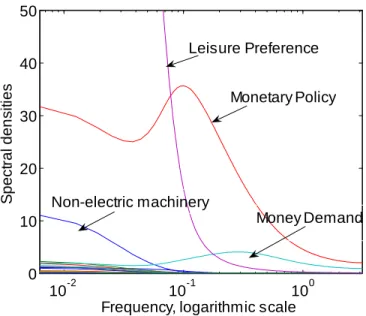
Figure 4 shows the graphs of (1=2 ) jG1;k(!)j2: For some k; the spectral densities are

particu-larly large while for others they are small. We indicate which innovation the dominating densities correspond to. For example, the low frequency component (less than one cycle per 20 quarters, which is about 15 years) of the …rst dynamic principal component of the data is strongly dominated by the leisure preference innovation. For business cycle frequencies, the monetary policy innovation becomes dominant.6

The sum of the areas under the graphs of Figure 4 corresponding to the monetary policy, the money demand and the preference innovations measure the variance of the projection of the …rst principal component on the space spanned by all lags and leads of the corresponding economy-wide shocks. Such a variance constitutes 97.6% of the overall variance of the …rst dynamic principal component.

For the second dynamic principal component, the variance of its projection on the space spanned by all lags and leads of the economy-wide shocks is still a respectable 82.6% of its overall variance. However, for the third dynamic principal component, this number is much smaller: 16.8%. In fact, most of the variance of the third dynamic principal component is explained by the innovations to 6_{The logarithmic scale of the horizontal axis of the graph creates the impression that the …rst dynamic principal}

component of the data is totally dominated by the leisure preference innovation, which is not the case. The monetary policy innovation explains a comparable portion of the variance of the …rst dynamic principal component to that explained by the preference innovation.

10-2 10-1 100 0 10 20 30 40 50

Frequency, logarithmic scale

S pect ral den sit ies Leisure Preference Monetary Policy Money Demand Non-electric machinery

Figure 4: Spectal densities of the projections of the …rst dynamic principal component on the spaces spanned by all lags and leads of the innovations "t;k with k = 1; :::; 33:

the agricultural, coal mining and textile mill productivity shocks. The variance of its projection on all lags and leads of these shocks constitutes 67.0% of its overall variance.

Hence, as we had qualitatively expected, the projection of the two …rst dynamic principal components on the space spanned by all lags and leads of the economy-wide shocks is not much di¤erent from the dynamic principal components’s themselves. However, the economy-wide content of the third dynamic principal component is very weak. It should be noted here that the …rst two dynamic principal components explain 80.6% of the variance of the data-generating process while the share of the third dynamic principal component is only 2.4%. Therefore, the agricultural, coal mining and textile mill production shocks do not really have much in‡uence on the economic dynamics as might appear from their substantial share in the dynamics of the third dynamic principal component. The point we would like to stress is simply that the space of the lags and leads of the …rst three dynamic principal components is substantially di¤erent from the space of the lags and leads of the economy-wide shocks ft:

Can we interpret the …rst dynamic principal component as a univariate index summarizing the most relevant information in the history of the economy-wide shocks? The answer to this question depends on whether the projection of the …rst dynamic principal component on the space spanned by leads only of the economy-wide innovations is reasonably small. Let G1;k(!) =

(1=2 )P1_{s= 1}G1;k;se is! be the Fourier expansion for G1;k(!) : Let us de…ne G+_1;k(!) (1=2 )X1 s=0G1;k;se is! G_1;k(!) (1=2 )X 1 s= 1G1;k;se is!_:

Then, the variance of the projection of the …rst dynamic principal component on the leads only of the economy-wide innovations equals

(1=2 ) Z

G_1;mp(!)2+ G_1;md(!)2+ G_1;lp(!)2 d!;

where k = mp; md and lp for monetary policy, money demand and leisure preference shock inno-vations, respectively. We have computed this number: It equals 33.5% of the variance in the …rst dynamic principal component which is due to both the leads and the lags of the economy-wide innovations. The largest part of this percentage (69.9% of it) comes from f_1;lp(!)2: That is, the …rst dynamic principal component has a relatively large projection on the subspace spanned by the future of the leisure preference shock. This …nding suggests that in actual applications, the …rst dynamic principal component may be an imperfect index of the information contained in history of aggregate shocks.

4.

Static factors and principal components

In practice, it is often assumed that the dependence of the observables on the factors can be captured by …nite lag polynomials. That is, it is assumed that the maximal order of the component polynomials of (s)(L) in Y_t(s) = (s)(L) ft+ e(s)t is …nite and equal to, say, h: This assumption

allows researchers to represent the dynamic factor model in static form by interpreting the h lags of the dynamic factors as additional “static factors”. Then, the static principal components or the generalized principal components (see Forni et al., 2005) can be used to recover the static factor space. One advantage of such an approach relative to the dynamic principal components method is that the obtained estimates of the factor space are guaranteed to be orthogonal to the space of the future factor innovations and hence, can be used for forecasting.

The …rst question we address in this section is whether a few lags of ft capture most of the

information about Y_t(s) contained in (s)(L) ft: One way to answer this question is to repeat the

above pervasiveness analysis with (s)(L) replaced by a …nite lag polynomial matrix ~ (L) : We de…ne ~ (L) so that the coe¢ cients of its components ~ij(L) = ~ij;0+ ~ij;1L + ::: + ~ij;hLh equal

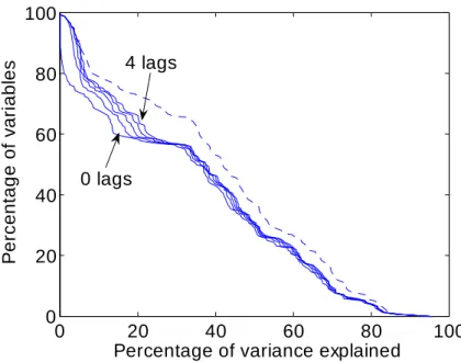
the coe¢ cients of the linear projection of Y_it(s) on fjt; fj;t 1; :::; and fj;t h. Figure 5 reports the

pervasiveness graph (dashed line) for the leisure preference shocks copied from Figure 1 superim-posed with the “…nite-lag pervasiveness graphs”for di¤erent values of h = 0; 1; 2; 3 and 4: Precisely,

0 20 40 60 80 100 0 20 40 60 80 100

Percentage of variance explained

P ercentag e of v ariabl es 0 lags 4 lags

Figure 5: Pervasiveness of the e¤ect of few lags only of the leisure preference shock on the observ-ables.

we plot the graphs of the …nite-lag pervasiveness functions ~ylp(z) de…ned as the percentage of the

components Y_it(s) of Y_t(s) for which the variance of the linear projection on the space spanned by flp;t; :::; flp;t h constitutes at least z% of the total variance of Y_it(s):

Note that the area under the graph (divided by 1002) equals the average fraction of the variance of Y_it(s)explained by ~i;lp(L) flp;t with the average taken over i = 1; 2; :::; 156: We see that, in terms

of the explanatory power, not much is lost by projecting the observables on the contemporaneous only (h = 0) leisure preference shock. To see this, compare the dashed and solid lines. As h increases, small improvements to the explanatory power take place. The largest improvement corresponds to the transition from h = 0 to h = 1:

Most of the changes to the graphs as h rises happen for y > 60: The reason is that this section of ordinates happens to correspond to sectoral in‡ations (section with y > 80) and sectoral wages (80 > y > 60). The contemporaneous leisure preference shock has essentially zero explanatory power for all the in‡ation indexes and very little explanatory power for sectoral wages. However, the one-period lagged leisure preference shock captures almost all the e¤ect (still very small) of the entire history of the leisure preference shocks on in‡ation (the one-lag graph almost coincides with the dashed line when y > 80). It also considerably helps to explain the level of wages.7

7

It is likely that one lag of the leisure preference shock would have almost as much of the explanatory power as the entire history of the leisure preference shock for the wage in‡ations (as opposed to the wage levels). We, however,

0 20 40 60 80 100 0 20 40 60 80 100

Percentage of variance explained

P ercentag e of v ariabl es 0 lags 4 lags

Figure 6: Pervasivenss of the e¤ect of few lags only of the monetary policy shock on the observables.

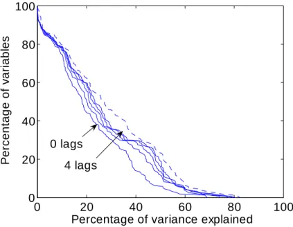
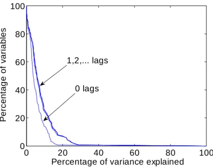
Figures 6 and 7 are the equivalents of Figure 5 for the monetary policy and the money demand shocks, respectively. The improvement in the explanatory power when h increases from 0 to 1 is more substantial than in the case of the leisure preference shock. However, further increases in h do not increase the explanatory power of the monetary policy factor much and do not increase the explanatory power of the money demand factor at all. Overall, we conclude that replacing the entries of (s)(L) with …nite lag polynomials so that the entries corresponding to the leisure preference shock become scalars and the entries corresponding to the monetary policy and money demand shock become polynomials of degree one, would not do much harm to the explanatory power of (s)(L)ft:

From the empirical perspective, our results provide support for the strategy of using a parsimo-nious number of lags to summarize the information about the observable variables that is contained in (L) ft for the purpose of factor extraction and forecasting. However, the “correct” number of

lags is an open question that requires the development of appropriate information criteria.

have included the levels rather than di¤erences of wages in our dataset. As a result, there is a large discrepancy between the solid lines and the dashed line in the 80 > y > 60 range of Figure 5.

0 20 40 60 80 100 0 20 40 60 80 100

Percentage of variance explained

P ercentag e of v ariabl es 0 lags 1,2,... lags

Figure 7: Pervasivenss of the e¤ect of few lags only of the money demand shock on the observables.

4.1 The content of the principal components

Since, as we saw above, only a very few lags of ftsubstantially add to factors’explanatory power, we

can approximate the dynamic factor decomposition (4) by the following static factor decomposition. Let mpt; mdtand lptdenote the monetary policy, money demand and leisure preference components

of ft: We de…ne a vector of static factors Ft as

Ft= (mpt; mpt 1; mdt; mdt 1; lpt)0

and write:

Y_t(s)= Ft+ t;

where ( i1; i2) is the vector of the coe¢ cients of the linear projection of Yit(s) on mpt and mpt 1;

( i3; i4) is the vector of the coe¢ cient of the linear projection of Yit(s)on mdt and mdt 1; and i5

is the coe¢ cient of the linear projection of Y_it(s)on lpt. We do not include lpt 1 into Ft because, as

can be seen from Figure 5, the lag of the leisure preference shock has very little explanatory power in our model. The lags of the monetary policy and money demand shocks have larger explanatory power and we include them into Ft:

In practice, Ft is not observed, and the space spanned by its components is estimated by the

2 4 6 8 10 12 14 0 0.2 0.4 0.6 0.8 1

Number of principal components

V ari anc e of th e proj ec ti on on the P C s pac e Leisure preference Monetary policy Money demand

Money demand lag Monetary policy lag

Figure 8: Portion of the variance of di¤erent components of the vector of static factors Ft

ex-plained by the projection on the spaces spanned by the …rst several (static, population) principal components.

the two spaces. We focus on the population principal components to see what the theoretical limit to the principal-component-based estimation of Ft is.

We would expect the principal components work well if all …ve non-zero eigenvalues of E (FtFt0) 0

are substantially above the largest eigenvalue of E _t 0_t: Unfortunately, this is not the case. Our computations show that the eigenvalues of E (FtFt0) 0 equal 64.54, 30.49, 5.45, 1.46, and 0.003.

But the largest eigenvalue of E _t 0_tequals 21.68, which is larger than three out of the …ve eigenvalues of E (FtFt0) 0:

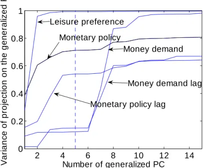
Then, what do the …rst …ve population principal components of Y_t(s) correspond to? Figure 8 reports the variances of the projections of the components of Ft(normalized to have unit variance

each) on the space spanned by the …rst r population principal components of Y_t(s) as functions of r: Had the space of the …rst …ve principal components spanned the same space as the components of Ft; the variances of the projections would each be equal to one at r = 5.

From the …gure, we see that the spaces spanned by the components of Ft and by the …rst …ve

principal components are substantially di¤erent. Only the leisure preference shock component of Ftis accurately “recovered”by the principal components. The money demand shock content of the

starts to be non-trivially present in the principal components’ space when r becomes larger than six.

A possibility remains that the …rst …ve principal components span the same space as …ve lin-ear …lters of ft; which are di¤erent from the mpt; mpt 1; mdt; mdt 1 and lpt that we (somewhat

subjectively) chose above to represent static factors. That this possibility does not realize can be seen from the following calculation. We compute the proportions of the variances of the …rst …ve principal components explained by their projections on the space spanned by the entire history of ft: The computed proportions turn out to be: 96.6%, 98.3%, 80.8%, 76.9%, and 24.6% for the …rst,

second, third, fourth, and …fth principal components, respectively.8 _{Therefore, the …fth principal}

component has very little to do with the history of the economy-wide shocks. 4.2 The content of the generalized principal components

In this section, we would like to know whether the space of the generalized principal components proposed by Forni et al. (2005) better match the space of Ft than the space of the static principal

components. Recall that the (population) generalized principal components are de…ned as follows. Let SY (!) be the spectral density matrix of the standardized data and let j(!) and pj(!) be

its j-th largest eigenvalue and the corresponding unit-length row eigenvector, respectively, so that pj(!) SY (!) = j(!) pj(!). Consider the sums

S (!) q X j=1 j(!) pj(!)0pj(!) S (!) n X j=q+1 j(!) pj(!)0pj(!)

where q is the number of dynamic factors, and compute

0 = Z S (!) d! 0 = Z S (!) d!:

We set q = 3 because there are three economy-wide shocks in the model. Then, the j-th (population) generalized principal component of Y_t(s) relative to the couple ₀; ₀ is de…ned as ZjYt(s); where

Zj are the solutions of the generalized eigenvalue equations

Zj 0 = jZj 0; (5)

8_{Compare these to the proportions of the variances of the …rst …ve principal components explained by their}

2 4 6 8 10 12 14 0 0.2 0.4 0.6 0.8 1 Number of generalized PC V ari anc e of proj ec ti on on the gen eral iz ed P C Leisure preference Monetary policy Money demand

Money demand lag Monetary policy lag

Figure 9: Portion of the variance of di¤erent components of the vector of static factors Ftexplained

by the projection on the spaces spanned by the …rst several (population) generalized principal components.

for j = 1; 2; :::; n, with the normalization constraints Zj 0Zj0 = 1 and Zi 0Zj0 = 0 for i 6= j; and

with 1 2 ::: n:

For our data generating process, the problem (5) is ill-posed in the sense that very small changes in ₀ may result in large changes in the solutions. This is so because the matrix ₀ turns out to have a large number of eigenvalues numerically close to zero. One way to proceed, which Forni et al. (2005) choose to follow, is to replace ₀ by the matrix with the same diagonal, but with zero o¤-diagonal elements. We do such a replacement in what follows.

Figure 9 is the equivalent of Figure 8 for the case of the generalized principal components. The two …gures are very similar. The proportions of the variances of the …rst …ve generalized principal components explained by their projections on the space spanned by the entire history of ftare equal

to 89.5%, 93.2%, 55.9%, 55.9% and 5.5%. These …gures suggest somewhat smaller macroeconomic content of the generalized principal components relative to the static principal components, for which the analogous …gures reported above are: 96.6%, 98.3%, 80.8%, 76.9%, and 24.6%.9

We conclude this section by summarizing its main …nding: for our data generating process, 9

The proportions of the variances of the …rst …ve generalized principal components explained by their projections on the space spanned by mpt; mpt 1; mdt; mdt 1and lptonly are: 73.3%, 91.9%, 42.1%, 38.4%, and 4.5%. Compare

the information about the space of the macroeconomic shocks and their most important lags is scattered through a relatively large number of principal components. Knowing the …rst …ve principal components is not su¢ cient to accurately recover the …ve shocks and lags. Knowing more principal components helps such a recovery. For example, in our exercises, the portion of the variance of the money demand shock and its lag explained by their projections on the space spanned by the …rst r principal components increase from below 20% for r = 5 to more than 60% for r = 7 or (in case of the generalized PC) r = 8: The principal component space of the same dimension as the number of shocks and their important lags may poorly approximate the “macroeconomic space”.

5.

Number of factors

The true number of factors may be interpreted in many di¤erent ways in the DSGE model of Bouakez et al. (2009). In this sense, the model replicates the same ambiguity that we …nd in actual applied research. Depending on the goal of the analysis, we might want to estimate di¤erent number of factors. Sometimes, the relevant goal of the analysis is to determine the number of basic macroeconomic shocks in‡uencing the dynamics of a large number of macroeconomic indicators. In this section, we therefore ask the following question. What is the relationship between the number of dynamic factors estimated from the data simulated from the model and the number of the economy-wide shocks in this model, which is three?

We use the Bai-Ng (2007) and Hallin-Liska (2007) criteria to estimate the number of factors in 1000 di¤erent simulations of our data with n = 156 and T = 120. Before applying the criteria, we demean and standardize the simulated data. First, we apply the Hallin-Liska (2007) method. The choice of the tuning parameters of the Hallin-Liska method is as follows. In Hallin and Liska’s (2007) notation, we use the information criterion IC_2;nT with penalty p1(n; T ); set the truncation

parameter MT at

h

0:7pTi and consider the subsample sizes (nj; Tj) = (n 10j; T 10j) with

j = 0; 1; 2; 3 so that the number of the subsamples is J = 4: The cross-sectional units excluded from the subsamples are determined randomly. We chose the penalty multiplier c on a grid 0:01 : 3 wiht increment 0:01 using Hallin and Liska’s second “stability interval”procedure. We applied the Hallin-Liska method to 1000 di¤erent simulations of our data, choosing the subsamples randomly each time and setting the maximum number of dynamic factors at 8. Out of 1000 times, the method …nds one dynamic factor 4 times, two dynamic factors 100 times, three dynamic factors 274 times, four dynamic factors 259 times, …ve dynamic factors 180 times, six dynamic factors 109 times, and seven dynamic factors 74 times.

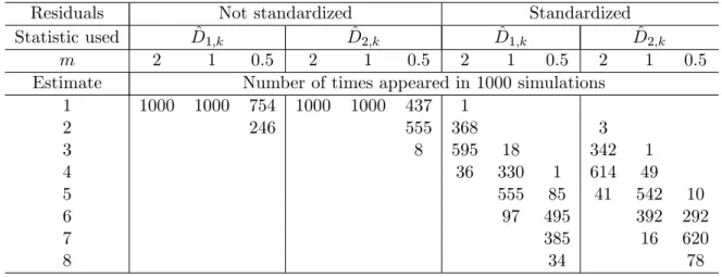
Next, we use the Bai-Ng (2007) method to determine the number of dynamic factors. We set the maximum number of static factors at 10; and, in the notation of Bai and Ng (2007), use either

^

D1;k or ^D2;k statistic for either the residuals or the standardized residuals of a VAR(4) …tted to

the estimated factors, and consider = 0:1 and m = 2; 1 and 0:5. Table 1 summarizes our …ndings for di¤erent choices of the tuning parameters.

Table 1: Number of times di¤erent estimates of the number of factors appeared in 1000 simulations

Residuals Not standardized Standardized

Statistic used D^1;k D^2;k D^1;k D^2;k

m 2 1 0.5 2 1 0.5 2 1 0.5 2 1 0.5

Estimate Number of times appeared in 1000 simulations 1 1000 1000 754 1000 1000 437 1 2 246 555 368 3 3 8 595 18 342 1 4 36 330 1 614 49 5 555 85 41 542 10 6 97 495 392 292 7 385 16 620 8 34 78

Bai and Ng estimates based on the standardized residuals are less conclusive than their estimates based on raw residuals, which suggest that there is one, or perhaps, two dynamic factors in the data. When the standardized residuals are used in the Bai and Ng procedure, the estimated number of dynamic factors depends very much on the parameter m; which regulates the scale of the threshold below which the eigenvalues of the sample correlation matrix of residuals are interpreted as small enough to conclude that the corresponding eigenvalues of the population correlation matrix of the errors of the VAR(4) equal zero. The dependence of the conclusions on the choice of the threshold was the motivation for Hallin and Liska to design their second stability interval procedure. In our Monte Carlo experiment, the Hallin-Liska estimates of the number of factors vary, the most frequent estimates being three, four and …ve dynamic factors.

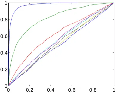
Finally, we test di¤erent hypotheses about the number of dynamic factors using Onatski’s (2009) test. Figure 10 reports the cumulative empirical distributions of the p-values computed in 1,000 Monte Carlo experiments for the test of 0 factors vs. 1 factor, 1 factor vs. 2 factors, 2 factors vs. 3 factors, and so forth. The steeply increasing cumulative distribution function (c.d.f.) corresponds to the null of zero factors, which indicates that the probability of rejection of this null is much larger than the size of the test. The next steepest c.d.f. is for the null of one factor. Note that we are still rejecting the null hypothesis with probability much larger than the size. The third steepest c.d.f. is not steep. So if we were to perform the test in a single “typical”monte Carlo simulation of the data, we would likely accepted either the hypothesis of one dynamic factor, or the hypothesis

0 0.2 0.4 0.6 0.8 1 0 0.2 0.4 0.6 0.8 1

Figure 10: The Monte Carlo cumulative empirical distributions of the p-values for Onatski’s (2009) test of 0 factors vs. 1 factor, 1 factor vs. 2 factors, 2 factors vs. 3 factors, etc.

of two dynamic factors.

All the above methods of the determination of the number of factors are based on the idea that the number of exploding eigenvalues of the spectral density matrix of the data as n ! 1 equals the true number of factors. However, as Figure 3 shows, only two of the “economy-wide eigenvalues“ are larger than the largest “idiosyncratic eigenvalue”. Hence, whenever the above criteria estimate more than two factors, the reason for such an estimate is not that the criterion is sensitive enough to detect the third macroeconomic shock from the noisy signal. The reason is simply that the criterion classi…es some sector-speci…c sources of variation as in‡uential enough to call them factors.

As was mentioned above, in practice, the dynamic factor models are often represented in the static form and then estimated by principal components. Before the estimation, the number of static factors should be determined. As in the case of the dynamic factors, the number of static factors can be interpreted in many di¤erent ways, and di¤erent loss functions imply di¤erent optimal estimates of this number. If the goal is to determine the number of macroeconomic shocks and their lags which su¢ ce to accurately describe the systematic components of the data, then, perhaps, the desired estimate is …ve as discussed above.

A basic informal method for the determination of the number of factors was proposed by Cattel (see Cattel, 1966). It uses the visual analysis of the scree plot, which is the line that connects the

1 2 3 4 5 6 7 8 9 10 11 12 13 14 15 0 0.2 0.4 0.6 0.8 1 No rm a liz e d v a lu e s Eigenvalue order

Sample distribution of the scree plot

Figure 11: Monte Carlo distribution of the scree plot for the data simulated from the BCR model.

decreasing eigenvalues of the sample covariance matrix of the data plotted against their respective order numbers. In practice, it often happens that the scree plot shows a sharp break where the true number of factors ends and “debris” corresponding to the idiosyncratic in‡uences appears.

Figure 11 shows the 15 largest eigenvalues (normalized so that the largest eigenvalue is 1) of the sample correlation for our simulated dataset. The boxplots represent the sample distribution of the 15 largest eigenvalues (based on 1000 Monte Carlo simulations). By looking at the scree, a researcher would sometimes think that there is only one static factor in the data and sometimes that there are two or three such factors.

Next, we apply Bai and Ng’s (2002) criteria P Cp1; P Cp2; P Cp3; ICp1; ICp2; ICp3; and BIC3;

and Onatski’s (2005) ED criterion to determine the number of static factors in each of the 1,000 Monte Carlo simulations of our data generating process (DGP).10 We consider three choices of the maximum number of static factors: rmax = 5; rmax = 10 and rmax = 15: For all the three choices,

the criteria P Cp1; P Cp2; P Cp3; ICp1; ICp2 and ICp3 estimate the number of static factors equal

to rmax: Criteria BIC3 and ED produce estimates which are smaller than rmax in most of the

considered cases.

The sample distributions of the estimates corresponding to BIC3 and ED (in the Monte Carlo

sample of 1,000 simulations) are shown in Figure 12. The number of factors estimated by BIC3; 1 0

0 5 10 15 0 500 ED r max=5 0 5 10 15 0 500 r max=10 0 5 10 15 0 500 r max=15 0 5 10 15 0 500 1000 B IC 3 0 5 10 15 0 500 1000 Number of factors 0 5 10 15 0 500 1000

Figure 12: The Monte Carlo distributions of the BIC3 and ED estimates of the number of static

factors.

although smaller than rmax in most of the cases, still very much depends on rmax: In contrast, the

results of ED are rather insensitive to rmax: In most of the Monte Carlo experiments, the number

of static factors estimated by ED is either 2 or 3.

Our …ndings so far can be summarized as follows. For our DGP, the economy-wide shocks do have a pervasive e¤ect on a large number of generated variables. However, the e¤ects of these shocks are not heterogeneous enough to identify the space of the macroeconomic ‡uctuations with the space of the few linear …lters of the data explaining most of its variance. Although most of the common dynamics of the data can be explained by the current economy-wide shocks and a very few of their lags, the space spanned by these shocks and lags is substantially di¤erent from the space of the population principal components of the same dimensionality. The …rst few of the principal components depend almost entirely on the macroeconomic shocks and their lags. However, the more distant principal component have a large sector-speci…c content. The information about the space of the economy-wide shocks and their lags is spread through a relatively large number of the population principal components.

6.

Sample

vs. population principal components

In practice, factors are estimated by sample principal components. Hence, even if the spaces of factors and population principal components coincided, there would be a discrepancy between the true and estimated factor space because sample and population principal components di¤er. In this section, we ask how large such a discrepancy would be for our data generating process. To answer this question, we rede…ne the true static factors of our standardized data as their population principal components. That is Fjt= (1=p 0j)v0j0 Y

(s)

t ; where 0j is the j-th largest eigenvalue and

v0j is the corresponding eigenvector of the population covariance matrix of Yt(s): As before, we

simulate 1,000 datasets Y1; :::; Y120: For each simulation, we compute matrix ₁₂₀1 P120_t=1Yt(s)Yt(s)0, its

eigenvalues j and the corresponding eigenvectors vj.11 Then the sample principal components are:

^

Fjt= (1=

p

j)vj0Y (s)

t : They estimate the “true” static factors Fjt: 6.1 Regressions of ^F on F

First, for each of ^F1t; :::; ^F6t, we compute the average R2 in the regression of ^Fjt on the constant

and F1t; :::; F6t. For j = 1; :::; 6; the corresponding numbers are: 1, 1, 0.98, 0.91, 0.73, and 0.57. We

clearly see that the more distant static factors are more poorly estimated. When we regress ^Fjt on

Fjt and a constant only, we get the following average R2 for j = 1; :::; 6: 0.89, 0.65, 0.67, 0.49, 0.22,

and 0.16. Note that the higher average R2 in the regressions of ^Fjt on F1t; :::; F6t relative to the

regressions of ^Fjt on Fjt is not a consequence of the fact that the “true”static factors are identi…ed

only up to a non-singular transformation. In our case, they are identi…ed up to a sign because we de…ne them as the population principal components. This phenomenon deserves further serious exploration, which we leave for future research.

The substantial decrease in the R2 with j in the individual regressions of ^Fjt on Fjt is consistent

with Onatski’s (2005) …nding that the coe¢ cient in the regression of a principal component estimate of a weak factor on the factor itself is substantially biased towards zero. The weaker the factor, the larger the bias and the smaller the R2:

6.2 Accuracy of the asymptotic approximation

Next, we consider the accuracy of Jushan Bai’s (2003) asymptotic approximation to the …nite sample distribution of ^Ft = F^1t; :::; ^Fkt

0

. Let X be an n by T matrix of our simulated stan-1 stan-1_{In practice, the standardized data would be obtained by using estimated standard deviations of the raw data}

series. Here, however, we abstract from this fact and use Yt(s);which are standardized by the true standard deviations.

This allows us to focus on the di¤erence between the population and sample principal components caused only by the di¤erence between the eigenstructures of EYt(s)Y

(s)0 t and 1 120 P120 t=1Y (s) t Y (s)0 t :

dardized data h

Y₁(s); :::; Y_T(s) i

. Let Ft = (F1t; :::; Fkt)0 be the true factors de…ned as the

popula-tion principal components, let F = [F1; :::; FT]0, and let 0 be the true factor loadings, that is 0 _{= [}p

01v01; :::;p 0kv0k]: Bai’s Theorem 1 says that, as long as certain asymptotic regularity

conditions are satis…ed12 and p_{n=T ! 0; for each t; we have:} p n F^t Hn;T0 Ft d ! N (0; t) ; (6) where Hn;T 00 0 n F0F^ T V 1 nT ;

VnT diag ^1; :::; ^k is the diagonal matrix of the …rst k of the largest eigenvalues of XX0= (nT ) ; t= V 1Q tQ0V 1; V is the diagonal matrix of eigenvalues of 1=2 F 1=2; F being the

probabil-ity limit of F0F=T and being the probability limit of 00 0=n; Q = V1=2 0 1=2 with having columns equal to the normalized eigenvectors of 1=2 F 1=2; t= limn!1(1=n)Pni=1

Pn j=1 0i 00j Ee (s) it e (s) jt

and e(s)_it are the idiosyncratic components in the factor model. In fact, the above asymptotics used in our setting implies that

p

n F^t Hn;T0 Ft p

! 0: (7)

This is because t = 0: Indeed, let us denote the matrix [v01; v02; :::; v0k] as V0k and the matrix

diag ( 01; 02; :::; 0k) as S0k: Then, 0 = V0kS 1=2 0k and Ft = S 1=2 0k V0k0 Y (s)

t : Since n is …xed (but

large) in our experiment, we cannot meaningfully take the limit of (1=n)Pn_i=1Pn_{j=1 i}0 00_j Ee(s)_it e(s)_jt as n ! 1: The best we can do is to set t = (1=n)Pn_i=1Pn_j=1 0i 00j Ee

(s) it e (s) jt : But Ee (s) t e(s)0t = E Y_t(s)Y_t(s)0 V0kS0kV_0k0 : Therefore, t = (1=n) 0 0h E Y_t(s)Y_t(s)0 V0kS0kV0k0 i 0 = (1=n)S_0k1=2V_0k0 hE Y_t(s)Y_t(s)0 V0kS0kV0k0 i V0kS_0k1=2 = (1=n)S_0k1=2hS_0k1=2E FtFt0 S 1=2 0k S0k i S_0k1=2 = (1=n)S0k E FtFt0 Ik S0k= 0:

We can check how accurate the asymptotic approximation (7) is in our case. Following the above Monte Carlo structure, we simulated 1,000 datasets and computed pn F^t H_n;T0 Ft for

each Monte Carlo replication. Figure 13 shows the median, and the 25 and 75 percentiles of the empirical distribution of the 1,000 Monte Carlo replications of pn F^t Hn;T0 Ft when only one

factor is estimated. We see that the approximation (7) works very poorly. Not only the interquartile 1 2

0 20 40 60 80 100 120 -3 -2 -1 0 1 2 3

MC percentiles of factor estimation error

time

Figure 13: The interquartile range and the median of the empirical distribution of the 1,000 Monte Carlo replications of pn F^t H_n;T0 Ft :

range of the empirical distribution of the Monte Carlo replications is wide, the distribution also has very fat tails in the sense that the moments of this distribution are large. For example, the standard deviation ofpn F^t Hn;T0 Ft is more than 4 for most of t = 1; 2; :::; 120:

Of course, if a researcher only had data simulated from our model but did not know the model itself, she would not know that t= 0 and would estimate it. In his Monte Carlo experiments, Bai

(2004) estimates t by ^t= VnT1(1=n)

Pn

i=1^e2it^i^0iV 1

nT ; where ^eit= Xit ^iF^t0 and ^0 = ^F0X=T:

To assess the quality of the asymptotic approximation (6), Bai (2004) computes the standardized estimate

gt= ^t1=2

p

n F^t Hn;T0 Ft (8)

and compares the empirical distribution of gt(for a …xed t) with the standard normal distribution.

We use Bai’s strategy below. For the moment, we consider the case of only one factor. One problem with such an exercise would be a double (imperfect) cancellation of errors. The quantity p_{n F^}

t Hn;T0 Ft would not be close to zero as we saw from Figure 13, but ^t will also be far

from zero because (1=n)Pn_i=1^i^0i^e2it would not be close to (1=n)

Pn i=1 Pn j=1 0i 00jEe (s) it e (s) jt since

the cross-sectional serial correlation is ignored and since T is not much larger than n:

When we plot the median and 25% and 75% percentiles of the Monte Carlo distribution of gtas

-150 -10 -5 0 5 10 15 0.1

0.2 0.3 0.4

Standardized factor error estimate vs. N(0,1)

Figure 14: The Monte Carlo distribution of g60relative to the distribution of the standard normal

random variable.

save space, we do not report this graph. Instead, we show the histogram for the 1,000 replications of ft when t = T =2 = 60 on Figure 14. The histogram is scaled so that the sum of the areas of all

the bars equals 1 and interimposed with the standard normal density.13

When several factors are estimated, the situation remains bad. The way in which the asymptotic approximation is not accurate varies with the explanatory power of the factor. Figure 15 shows the histograms for the Monte Carlo distributions of the components of gt when four factors are

estimated. We see that the standard normal asymptotic approximation to the empirical distribution of g1t is relatively accurate, but the empirical distributions of g2t; g3t and g4t have progressively

fatter tails relative to the standard normal approximation. We link such a deterioration of the quality of Bai’s asymptotic approximation to the decreasing explanatory power of more distant factors.14

We conclude that the asymptotic theory of the principal components estimates available to date does not provide a good approximation to the distribution of the estimates for our data

1 3_{The range of the horizontal axis is truncated at [-15,15] to improve visibility.} 1 4

Onatski (2005) describes a di¤erent asymptotic approximation designed speci…cally for the case when the factors are weak, as seems to be the case in our present exercise. However, Onatski’s formulas are derived for the case of neither cross-sectional nor serial correlation in the idiosyncratic terms and cannot be used here. In our opinion, derivation of the alternative weak factor asymptotics for the case of correlated idiosyncratic terms is an important task. We leave it for future research.

-50 0 5 0.2 0.4 Factor 1 -100 0 10 0.2 0.4 Factor 2 -100 0 10 0.2 0.4 Factor 3 -100 0 10 0.2 0.4 Factor 4

Figure 15: Monte Carlo distributions of g1;60; g2;60; g3;60; and g4;60 relative to the theoretically

derived standard normal distribution.

generating process. To the extent that the data generating process we consider is similar to actual macroeconomic datasets, this …nding calls for a new asymptotic theory, perhaps, based on the assumptions which better correspond to the …nite sample situation.

7.

Di¤usion Index Forecasting

Large factor models are often used as statistical devices which motivate and explain di¤usion index forecasting. Stock and Watson (2002) propose the following factor model framework for forecasting variable yt+1 using a high-dimensional vector Yt of predictor variables:

yt+1 = (L) ft+ (L) yt+ "t+1 (9)

Yit = i(L) ft+ eit; (10)

where (L) ; (L) and i(L) are lag polynomials in non-negative powers of L, ftare a few

economy-wide shocks in‡uencing a economy-wide range of variables Yit, and E ("t+1jft; yt; Yt; ft 1; yt 1; Yt 1; :::) = 0:

It turns out that equations (9)-(10) …t in our theoretical model quite well. For example, if we set yt equal to output growth or to aggregate in‡ation, and if we set ft equal to the three-dimensional

vector of economy-wide shocks: the monetary policy, the money demand and the leisure prefer-ence shocks, then the linear forecasts of yt+1 based on the history of yt and ft are nearly

E (yt+1jft; yt; ft 1; yt 1; :::) 6= E (yt+1jft; yt; Yt; ft 1; yt 1; Yt 1; :::), the degree of the violation is

very small. Precisely, using the state space representation (1) for our model, we numerically com-pare the variance of the optimal forecast error "o_t+1 = yt+1 E (yt+1jft; yt; Yt; ft 1; yt 1; Yt 1; :::)

with the variance of the forecast error "t+1= yt+1 E (yt+1jft; yt; ft 1; yt 1; :::). For output growth

we …nd that

V ar (yt+1) V ar ("t+1)

V ar (yt+1) V ar "o_t+1

= 0:991; (11)

which means that the history of ytand ftalone captures 99.1% of all forecastable variance in yt+1:

For aggregate in‡ation, the corresponding …gure is 98.9%.

The reason why we use the above measure of forecast accuracy as opposed to, say, the mean squared forecast error ratio V ar ("t+1) =V ar "ot+1 is that in our model, output growth and

aggre-gate in‡ation are not easily forecastable. For example, for output growth, the ratio V ar "o

t+1 =V ar (yt+1)

equals 0.8484 (for in‡ation, the similar number is 0.8616) so that only 15.2% of the variance of output growth (and 15.8% of the variance of aggregate in‡ation) is forecastable at one quarter hori-zon. Therefore, had we used V ar ("t+1) =V ar "ot+1 as a measure of sub-optimal forecast accuracy,

any reasonable forecast would produce a number in between 1 and (0:8484) 1 = 1:179 (the latter number would correspond to zero forecast) making the measure not particularly informative.

In our model, the factors represented by the three economy-wide shocks have large forecasting power relative to other predictors. For example, the forecast of output growth based on its own history and the history of aggregate in‡ation captures 79% of the forecastable variance, whereas the forecast based on the history of ftalone captures 98.8% of the forecastable variance. For aggregate

in‡ation, its forecast based on the own history and the history of output growth captures 75.5% of the forecastable variance, whereas the forecast based on the history of ft alone captures 97.4%

of the forecastable variance. Hence, the di¤usion index forecasts substantially outperform small VAR forecasts in our model, at least theoretically. Further analysis of the predictive power of ft

shows that the forecasts based on the separate histories of the monetary policy shocks, money demand shocks and leisure preference shocks capture 47.8%, 46.6% and 4.4%, respectively, of the forecastable variance of output growth. For aggregate in‡ation, the similar numbers are 75.5%, 11.6% and 10.2%.

In practice, to implement (9)-(10), an important simplifying assumption that the lag polynomi-als (L), (L) and i(L) are of …nite order is usually made. Equation (10) is replaced by a static

factor representation: Yit= iFt+ eit; and equation (9) is replaced by

yt+1= 1+ 1(L)Ft+ 1(L) yt+ "t+1; (12)

by the sample principal components and the coe¢ cients of the above forecasting equation are estimated by ordinary least squares (OLS) of yt+1 on ^Ft; yt and a few of their lags.

We have already seen that the space of principal component is substantially di¤erent from the space of macroeconomic static factors represented by mpt; mpt 1; mdt; mdt 1 and lpt: There are

substantial di¤erences both at population and sample levels. At the population level, the macro-economic space is substantially di¤erent from the space of the population principal components. At the sample level, the sample principal components imperfectly estimate the space of the popu-lation principal components (but, as is seen from Figure 15, the discrepancy is mostly due to the estimation of the less in‡uential population principal components).

Although the di¤erence between the macroeconomic and principal component spaces may be harmful for structural analysis, it may not matter for di¤usion index forecasts. In this subsection, we explore this possibility in detail. We focus on the special case of (12):

yt+1= + 0Ft+ "t+1; (13)

with no lags of yt+1 and no lags of Ft as predictor variables. We set15

Ft= (mpt; mpt 1; mdt; mdt 1; lpt; lpt 1) : (14)

Let us denote the vector of the …rst six population principal components of vector Y_t(s)as P Ct;

and let us denote the vector of the …rst six sample principal components of Y_t(s); t = 1; :::; T; as d

P Ct: We estimate the coe¢ cients and in (13) by the OLS regression of yt+1; t = 1; :::; T 1

on a constant and dP Ct; and use the estimates to form the forecast:

^

y_{T +1jT} = ^ + ^0P CdT:

Then, we decompose the forecast error into four di¤erent parts as follows: yT +1 y^_{T +1jT} = yT +1 E (yT +1jYT; YT 1; :::) | {z } 1 + E (yT +1jYT; YT 1; :::) E (yT +1jFT) | {z } 2 + E (yT +1jFT) E (yT +1jP CT) | {z } 3 + E (yT +1jP CT) y^_{T +1jT} | {z } 4 : 1 5_{We have included lp}

t 1 in the set of static factors because, as was mentioned in the discussion of Figure 5, it