HAL Id: hal-00835023
https://hal-mines-paristech.archives-ouvertes.fr/hal-00835023
Preprint submitted on 24 Jun 2013HAL is a multi-disciplinary open access archive for the deposit and dissemination of sci-entific research documents, whether they are pub-lished or not. The documents may come from teaching and research institutions in France or abroad, or from public or private research centers.
L’archive ouverte pluridisciplinaire HAL, est destinée au dépôt et à la diffusion de documents scientifiques de niveau recherche, publiés ou non, émanant des établissements d’enseignement et de recherche français ou étrangers, des laboratoires publics ou privés.
How to simulate a volume-controlled flooding with
mathematical morphology operators?
Serge Beucher
To cite this version:
Serge Beucher. How to simulate a volume-controlled flooding with mathematical morphology opera-tors?. 2011. �hal-00835023�
How to simulate a volume-controlled flooding
with mathematical morphology operators?
Serge Beucher
CMM/Mines-ParisTech (November 2011) (Draft document, see copyright license)
Note: To follow this note and especially to get definitions of concepts as lower catchment
basin, FOZ, dual geodesic reconstruction, I STRONGLY recommend to read the following documents available on my Web page (http://cmm.ensmp.fr/~beucher/publi.html):
„ P algorithm, a dramatic enhancement of the waterfal transformation
(http://cmm.ensmp.fr/~beucher/publi/P-Algorithm_SB_BM.pdf, in particular, pages 1 to 10) [1]
„ Watersheds and waterfalls
(http://cmm.ensmp.fr/~beucher/slideshow/cours2000_fichiers/frame.htm) [2]
The problem
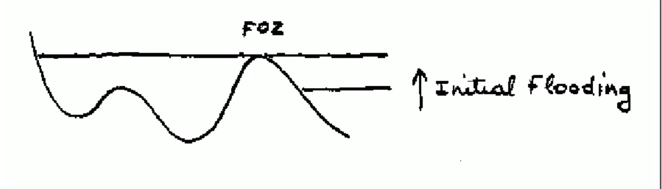
The classical tool for flooding simulation is the watershed transform. However, the flooding is simply controlled by its height. This means that, when the flooding has reached an altitude where it can flood an adjacent catchment basin (Fig 1), this catchment basin and also other catchment basins are immediately totally flooded up to the current level of water. In fact, the topography of these catchment basins has no importance since the flooding is immediate and not controlled by these catchment basins (Fig 2).
Fig 1: Flooding of the next CB is made immediately and totally. Several catchment basins may be flooded at the same time.
Fig2: The topography of the flooded catchment basins is not taken into account.
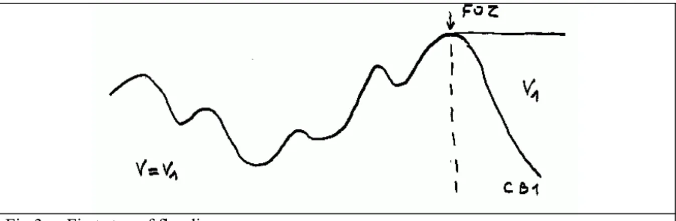
Simulating a volume-controlled flooding is not so simple as this process mixes two phenomena: a flooding phenomenon (identical to the flooding process occuring in the watershed transform) but also an overflow which occurs when the flood reaches the first
Fig 3-a: First step of flooding
At the first step, a volume V1 of water is used to flood the initial catchment basin CB1 up to
its first FOZ (Fig 3-a). The flooded region corresponds to the lower catchment basin LCB1
(see Fig 4 for a 2D illustration). Then, water pours through the FOZ and fills the adjacent catchment basin CB2 or, more precisely, the corresponding lower catchment basin LCB2. In
this case, the phenomenon which occurs is a waterfall rather than a flooding. At the end of this step, the volume of water which has been consumed is V1+V2. (Fig 3-b).
Fig 3-b: Flooding and flooded regions after step 2.
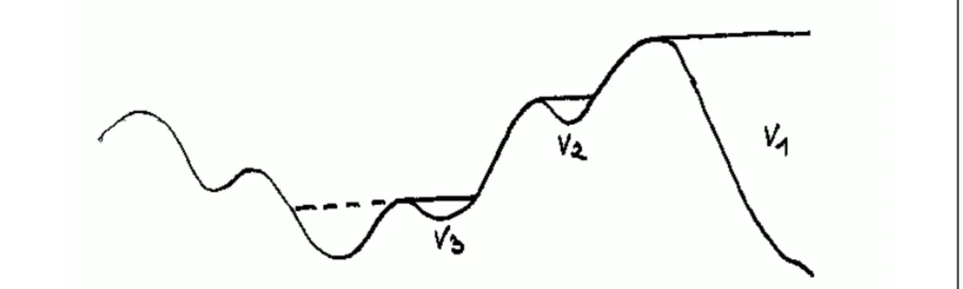
Then, the process goes on and at the third step, we obtain the result given at Fig 3-c. At the next step, the result of the flooding/waterfall process is illustrated at fig 3-d. The catchment basin CB4 is flooded from the previous one. However, the FOZ of this catchment basin sends
the flooding to the previous catchment basin CB3 which is already flooded! Therefore, the
flooding process must be continued in order to reach the FOZ connecting the already flooded regions and the first catchment basin not flooded yet (Fig 3-e).
Fig 3-d: Fourth step of flooding, intermediary result. If the next catchment basin is flooded up to its FOZ, the process is looping.
Fig 3-e: Fourth step, final result. The flooding process is continued until the next available FOZ is reached.
The next step is given at Fig 3-f.
Fig 3-f: Next step of flooding. Here again, the process must be continued after the intermediary flooding as no new FOZ is available.
Note that, when more than one catchment basin is flooded from a previous one, each new catchment basin is filled up to its own FOZ. This means that this procedure establishes, de facto, a flooding order or a hierarchy between the different catchment basins. The flooding of all the catchment basins adjacent to the previously flooded ones is synchronised. These catchment basins will not contribute to the next step of flooding until their corresponding lower catchment basins are all entirely flooded. We shall come back later to the consequences of this particular flooding scheme.
A flooding algorithm
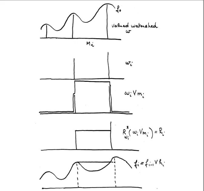
From the previous analysis, a volume-controlled flooding can be defined. Each step will be illustrated. We suppose that we have the initial valued watershed w of the DEM f0, the binary
image of all the catchment basins CB (which corresponds to the threshold at 0 of the valued watershed w). We also suppose, for the sake of simplicity, that the flooding source is unique and embedded in a single catchment basin (although there is no particular problem with this algorithm if this condition is not fulfilled).
At each step of the flooding, two objects will be built:
- the union Mi of all the catchment basins which have been involved in the flooding at step i
( involved means that these catchment basins have been reached by the flood but they are not necessarily totally flooded). Mi is, by construction, a single connected component (if
there is a single source of flooding).
- the flooded DEM fi after step i. The volume of water used at the end of this step
corresponds to the volume of (fi - f0).
The process is initialised by generating M1, made of the catchment basin containing the initial
source of flooding (Fig 4-a). Then the flooded topography f1 is built (see below how this can
be achieved). V1 = vol(f1 -f0) is the volume of water consumed in this first step. The
difference of these two functions corresponds to the lower catchment basin LCB1. It also
corresponds to the lower catchment basin of M1 (since at this step, M1 = CB1). Then, the FOZ
of this lower catchment basin is determined and the catchment basin adjacent to this FOZ in CB is added to M1 to produce M2. Note that M2 must be connected so the part of the
watershed line which separates M1 and the new catchment basin must be entirely removed.
We explain later how this is done.
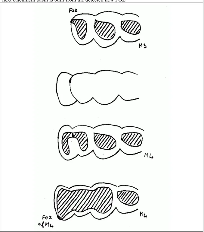
Fig 4-a: 2D representation of the process. Initial catchment basins and generation of M1
(CB1) from the flooding source. Then, the FOZ is determined by geodesic reconstruction.
The corresponding lower catchment basin is built and the next catchment basin is added (it is marked by the FOZ).
Fig 4-b: Second step. M2 is computed, the flooded corresponding region is determined, the next catchment basin is built from the detected new FOZ
Fig 4-c: Steps 3 and 4 of the process. At step 4, the intermediary result shows that there is no FOZ reached by the flood yet. Therefore, the flooding must be continued up to the FOZ belonging to the boundary of M.
The next step consists in determining the flooded topography f2. The supplementary flooded
zone is obviously contained into M2. Then, after the determination of the corresponding FOZ,
the adjacent catchment basin(s) is (are) added to M2 to produce M3. Fig 4-b and Fig 4-c
illustrate these different steps. Note the particular behaviour at step 4. In this case, as we have reached one of the lowest catchment basin, the next flood does not invade a new catchment basin but, on the contrary, it continues to spread into M4. This simply means that no waterfall
occurs anymore and that the classical watershed flooding is acting again.
At each step, the flooded volume can be calculated easily. We can then control this flooding by introducing a maximum available volume of water Vmax. If, after step i, the flooded
volume Vi is lower than Vmax, the process goes on. If not, we stop the process at the previous
step i-1. The difference of volume Vmax - Vi-1 can be managed easily since we know which
catchment basins should be partly flooded by this quantity of water (see below).
How to determine fi and the active FOZ at each step?
Determining fi and the current FOZ can be achieved with the geodesic reconstruction. In fact,
the procedure is similar to the algorithm which is used to build the hierarchical image (see page of [1] or slide in [2]). The only difference is that this procedure is not applied on the whole valued watershed but only on the part of it which corresponds to the boundary of Mi at
step i.
Let Mi be the (partly) flooded region at step i and mi its corresponding valued mask. The
operation:
w. [3(mi)− mi]= wi
gives the valued boundary of Mi.
The dual reconstruction of wi with wi-mi as marker function gives the local hierarchical
image of wi (hierarchical image limited to Mi):
hi= Rw&i(wi- mi)
fi is then equal to fi= fi−1- hi (Fig 5).
Fig 6: Successive steps of the construction of Mi+1.
Getting the FOZ of Mi is quite complicated. The procedure described in [1] is a good start but
it is not sufficient as some FOZ may be large (FOZ corresponding to triple points of the watershed).
Firstly, we determine the points for which 3(hi. mi)= wi. Let Z be this set and z the corresponding numerical mask. Then, we must iterate the following operations until
„ compute 3(wi. z)
„ generate Z= 3(wi. z) = wi and the corresponding numerical mask z. The determination of Mi+1 is obtained by:
Mi+1= R[SKIZ(Mi4 CB 4 Z),Mi]
Where SKIZ produces the zones of influence of the set (Mi4 CB 4 Z) and R is the geodesic reconstruction (Fig 6).
Algorithm description
Here are the different steps of this algorithm. Initial data:
- The DEM image f0
- The initial source of flooding, S (it is a set). - The maximum volume owater available, Vmax.
Initialisation
1. Compute w, the valued watershed of f0.
2. Generate the catchment basins image CB of w (set obtained by thresholding w at 0). 3. Compute M = build(CB, S) ; M is the set of all the (even partly) flooded catchment basins
at the end of each step.
4. Generate m (valued mask of M, obtained by a convert function). 5. Let the current flooded topography fi be equal to f0.
Process
1. fi−1= fi (fi-1 is the flooded topography at the beginning of each step).
2. M∏ = M (M indicates the partly flooded catchment basins at the beginning of each step). 3. Compute m (convert function applied to M )
4. Calculate wi= w . [3(m∏)− m∏]
5. Calculate hi= Rw&i(wi- m (dualbuild of over wi.
∏) (w
i- m∏)
6. Calculate fi= fi−1- hi
7. Calculate V = vol(fi - f0), total volume of water consumed since start.
8. Calculate Vi = vol(fi - fi-1), volume used at step i (optional).
9. Call getFOZ(m , wi, hi), result is the FOZ Z (see description of this function below).
10. Compute WRK1 = M∏4 CB 4 Z
11.WRK1= SKIZ(WRK1)
12. M = build(WRK1, M ), geodesic reconstruction.
13. If (V[ Vmax), then go to step 1 14. Else, end of flooding.
Procedure Z = getFOZ(m, w, h)
1. Determine points such that w= 3(h . m) and store them in Z. 2. Calculate z (numerical convert of Z).
3. v0 = vol(Z).
4. v1 = v0
5. Compute 3(w. z)
6. Put points such that 3(w. z) = w in Z 7. Calculate z
8. v0 = vol(Z)
9. If (v0 > v1) then go to step 4 10. End (Z contains the FOZ)
Mamba implementation
[to be done]
Comments
The above procedure requires some comments.
Firstly, it is more an ordering of the various catchment basins rather than a simulation of the flood. This procedure provides a kind of flooding graph which simply indicates which catchment basins (or unions of catchment basins) will be flooded next when a given catchment basin has been flooded. This corresponds to a hierarchy of catchment basins. However, the flooding/overflow procedure is synchronised. This means that the basins belonging to a same level of hierarchy will be flooded simultaneously only when all the catchment basins belonging to the previous level have been flooded (up to their respective FOZ). It is unlikely that a real flooding would follow this rule. We have, for instance, no control of the rate of flow in this procedure. This rate of flow will surely depend, in the real flooding process, of lots of factors: size of FOZ, dynamics of the flow (speed), etc. Moreover, when a small catchment basin is filled, neighbouring catchment basins will be flooded without waiting for the end of flooding of the other catchment basins belonging to the same hierarchy. Therefore, the calculation of the volume of water involved at each step of the above procedure may be biased and may not correspond to the real situation.
Secondly, this procedure does not simulate the flooding itself but it simply gives an idea of the result of this flooding, that is, the regions which could be affected by this flooding. Indeed, this information can be useful to establish risk maps.
Thirdly, the described procedure allows to know if the general flooding process is mainly achieved through a classical watershed-like flooding or through an overflow, by a very simple way illustrated at Fig 4-c (step 4): when at least two previously flooded regions merge, this means that the process is again a flooding process (a minimal catchment basin has been reached). On the contrary, if a new non connected flooded region appears, this region has been added through an overflow. At the end, the situation where the calculated volume of water corresponds to the real one involved is when the flooded surface is made of a single connected component as illustrated at Fig 1 (if only one flooding source is used).
It could be possible, then, to use the catchment basins hierarchy graph obtained by the above procedure to design another more realistic flooding schemes based on graph valuation and propagation. Although there exists morphological operators able to handle this kind of data structure (generalised geodesic operators), it is likely that these flooding schemes would also require the use of other mathematical and simulation tools.
This work is licensed under a Attribution-NonCommercial-NoDerivatives (CC BY-NC-ND) 3.0 Creative Commons License