independent data
C. Senten1, M. De Mazi`ere1, B. Dils1, C. Hermans1, M. Kruglanski1, E. Neefs1, F. Scolas1, A. C. Vandaele1, G. Vanhaelewyn1, C. Vigouroux1, M. Carleer2, P. F. Coheur2, S. Fally2, B. Barret3,*, J. L. Baray4, R. Delmas4, J. Leveau4, J. M. Metzger4, E. Mahieu5, C. Boone6, K. A. Walker6,7, P. F. Bernath6,8, and K. Strong7
1Belgian Institute for Space Aeronomy (BIRA-IASB), Brussels, Belgium
2Service de Chimie Quantique et Photophysique (SCQP), Universit´e Libre de Bruxelles (ULB), Brussels, Belgium 3formerly at: BIRA-IASB and SCQP/ULB
4Laboratoire de l’Atmosph`ere et des Cyclones (LACy), Universit´e de La R´eunion, France 5Institute of Astrophysics and Geophysics, University of Li`ege, Li`ege, Belgium
6Department of Chemistry, University of Waterloo, Waterloo, Ontario, Canada 7Department of Physics, University of Toronto, Toronto, Ontario, Canada 8Department of Chemistry, University of York, Heslington, York, UK *now at: Institut d’A´erologie, Toulouse, France
Received: 1 November 2007 – Published in Atmos. Chem. Phys. Discuss.: 17 January 2008 Revised: 23 April 2008 – Accepted: 20 May 2008 – Published: 2 July 2008
Abstract. Ground-based high spectral resolution
Fourier-transform infrared (FTIR) solar absorption spectroscopy is a powerful remote sensing technique to obtain information on the total column abundances and on the vertical distribution of various constituents in the atmosphere. This work presents results from two FTIR measurement campaigns in 2002 and 2004, held at Ile de La R´eunion (21◦S, 55◦E). These cam-paigns represent the first FTIR observations carried out at a southern (sub)tropical site. They serve the initiation of regu-lar, long-term FTIR monitoring at this site in the near future. To demonstrate the capabilities of the FTIR measurements at this location for tropospheric and stratospheric monitor-ing, a detailed report is given on the retrieval strategy, infor-mation content and corresponding full error budget evalua-tion for ozone (O3), methane (CH4), nitrous oxide (N2O), carbon monoxide (CO), ethane (C2H6), hydrogen chloride (HCl), hydrogen fluoride (HF) and nitric acid (HNO3)total and partial column retrievals. Moreover, we have made a thorough comparison of the capabilities at sea level altitude (St.-Denis) and at 2200 m a.s.l. (Ma¨ıdo). It is proved that the performances of the technique are such that the atmospheric variability can be observed, at both locations and in distinct
Correspondence to: C. Senten
altitude layers. Comparisons with literature and with cor-relative data from ozone sonde and satellite (i.e., ACE-FTS, HALOE and MOPITT) measurements are given to confirm the results. Despite the short time series available at present, we have been able to detect the seasonal variation of CO in the biomass burning season, as well as the impact of particu-lar biomass burning events in Africa and Madagascar on the atmospheric composition above Ile de La R´eunion. We also show that differential measurements between St.-Denis and Ma¨ıdo provide useful information about the concentrations in the boundary layer.
1 Introduction
The Network for the Detection of Atmospheric Composi-tion Change1 (NDACC, http://www.ndacc.org/) is a world-wide network of observatories, for which primary objectives are to monitor the evolution of the atmospheric composition and structure, and to provide independent data for the vali-dation of numerical models of the atmosphere and of satel-lite data. NDACC also supports field campaigns focusing on specific processes at various latitudes and seasons. Only 1This was formerly called the Network for the Detection of Stratospheric Change or NDSC.
a few stations in NDACC are situated in the tropical and subtropical belts. In particular, there are not yet any long-term Fourier transform infrared (FTIR) measurements in the Southern Hemisphere tropics. The only tropical NDACC stations at which FTIR measurements are performed are Mauna Loa (19.54◦N, 155.6◦W) and Paramaribo (5.8◦N, 55.2◦W), both in the Northern Hemisphere. The former one is at high altitude (3459 m a.s.l.), and at the latter one, the measurements are performed on a campaign basis, since September 2004 only (Petersen et al., 2008). Therefore, we have chosen the Observatoire de Physique de l’Atmosph`ere de La R´eunion (OPAR) to initiate such measurements. The OPAR is located at 21◦S, 55◦E, in the Indian Ocean, East of Madagascar, at the edge between the southern tropics and subtropics. It is a measurement station led by the Laboratoire de l’Atmosph`ere et des Cyclones (LACy) of the Universit´e de La R´eunion, that performs radio sonde observations since 1992, SAOZ measurements since 1993 and lidar measure-ments since 1994 (Baray et al., 2006). The implementation of FTIR solar absorption measurements at this site, providing information about the total column abundances and vertical distributions of a large number of atmospheric constituents (e.g., Brown et al., 1992), will therefore be a useful comple-ment to the station’s observations, and will fill the gap in the Southern Hemisphere tropical region.
In this paper, we present results from the first two FTIR campaigns that we performed at Ile de La R´eunion, in 2002 and 2004, to verify the feasibility of FTIR measurements at a tropical site and to start the long-term monitoring. Know-ing that water vapour is a strong absorber in the infrared and that there is a larger humidity at tropical sites than at mid-and high-latitude sites, especially at low altitude, it is impor-tant to characterize the capabilities of FTIR monitoring at a tropical location. During the first campaign we have made simultaneous measurements at two locations with an altitude difference of about 2.2 km, to compare the observation char-acteristics at these two altitudes. This campaign has also al-lowed us to make some differential measurements, charac-terizing the boundary layer. The second campaign was made at the lowest altitude site, to initiate the long-term measure-ments and to contribute to satellite validation, in particular of the Atmospheric Chemistry Experiment – Fourier Trans-form Spectrometer (ACE-FTS), onboard the Canadian satel-lite SCISAT-1 (http://www.ace.uwaterloo.ca).
The results presented here concern a number of species that have been selected for three main reasons: their im-portant roles in tropospheric or stratospheric chemistry, their link to current environmental problems like climate change or stratospheric ozone depletion, and the fact that they are needed for satellite validation. More specifically, our analyses focus on the primary greenhouse gases CH4, N2O and O3, on the secondary greenhouse gases CO and C2H6, and on HCl, HF and HNO3. Apart from their indirect effect on climate change, CO and C2H6play a central role in tropo-spheric chemistry through their reactions with the hydroxyl
radical OH (Brasseur and Solomon, 1984). They are emitted primarily by anthropogenic sources, and they can be used as tracers of tropospheric pollution and transport (e.g., transport of emissions from biomass burning), because they have rel-atively high tropospheric abundances and long tropospheric lifetimes.
In the stratosphere, HCl has a non-negligible impact on the ozone budget, acting as a reservoir species for chlorine. HF is a useful tracer of vertical transport, and of the anthropogenic emissions of fluorinated compounds.
HNO3is formed in the reaction of OH with NO2and plays an essential role as a reservoir molecule for both the NOx (nitrogen oxides) and HOx(hydrogen oxides) radicals, which are potentially active contributors to the ozone destruction in the stratosphere through catalytic reactions.
The results cover only short time periods, but their com-parison with literature data and with correlative measure-ments shown in the paper, demonstrate the potential of these measurements at Ile de La R´eunion. In particular, we show that the location of the site East of Africa and Madagascar of-fers interesting opportunities to observe transport of biomass burning emissions.
Sections 2, 3 and 4 describe the campaign characteristics, the retrieval method and the optimal retrieval parameters for every selected molecule individually. Section 5 presents the associated error budget calculations, together with a discus-sion of the resulting error estimations. Section 6 discusses the FTIR data as well as comparisons with correlative data. Conclusions and future plans are given in Sect. 7.
2 Specifications of the FTIR measurement campaigns
During the first FTIR solar absorption measurement cam-paign at Ile de La R´eunion, in October 2002, two almost identical instruments, i.e., mobile Bruker 120M Fourier transform spectrometers, were operated in parallel at two different locations. The one belonging to the Belgian In-stitute for Space Aeronomy (BIRA-IASB) was installed on the summit of the mount Ma¨ıdo (2203 m a.s.l., 21◦040S and 55◦230E), and the one from the Universit´e Libre de Bruxelles (ULB) at the nearby St.-Denis University campus (50 m a.s.l., 20◦540S and 55◦290E).
The BIRA-IASB instrument was placed in an air-conditioned container, and the electricity was provided with a power generator located south of the container. The so-lar tracker (purchased from Bruker) was mounted on a mast attached to the wall of the container, and the solar beam en-tered the container through a hole in that wall. The ULB instrument was installed in a laboratory of the university. Its solar tracker (also purchased from Bruker) was attached to the edge of the roof of the laboratory and the solar beam en-tered the room through a side-window.
During the second campaign, from August to Octo-ber 2004, we limited ourselves to one instrument from
automatic or remotely controlled way (Neefs et al., 2007). It has successfully been used during both campaigns with the BIRA-IASB instrument. The BARCOS system includes a meteorological station and a data logger to continuously monitor and log the local weather conditions as well as other housekeeping parameters, i.e., instrument and environment status. BARCOS executes a daily script that schedules and runs the measurements. It interrupts the observation sched-ule when the solar tracker is not capable of tracking the sun because of the presence of clouds, and it resumes the sched-ule once the sun re-appears. BARCOS automatically closes or opens the suntracker hatch when it starts or stops raining, respectively. Unfortunately, at the time of the campaigns, the automatic filling of the detector dewars with liquid nitrogen was not implemented yet, and hence it was not possible to operate the FTIR instrument without a person on site.
Both spectrometers allowed a maximum optical path dif-ference (MOPD) of 250 cm, providing a maximum spectral resolution, defined as 0.9/MOPD, of 0.0036 cm−1. Never-theless, to record the solar absorption FTIR spectra, we have not always used the maximum spectral resolution. The ac-tual resolution has been selected on the basis of the Doppler broadening of the lines and it has been lowered at high so-lar zenith angles, in order to reduce the measurement time. More specific information is given in Sect. 4. For all spectra, we have used a KBr beamsplitter in the interferometer, and one of six different optical bandpass filters in front of the de-tector, which is a nitrogen-cooled InSb (indium antimonide) or MCT (mercury cadmium telluride or HgCdTe) detector, according to the target spectral range. The optical filters are the ones used generally in the NDACC FTIR community. In particular, during the first campaign in 2002 we have used filters 1, 2, 3, 5 and 6, while during the second campaign in 2004 we have used filters 1, 2, 3, 4 and 6. So during the 2002 campaign the spectral region between 1400 and 2400 cm−1 has been covered using the MCT detector with the NDSC-5 filter (range 13NDSC-50–22NDSC-50 cm−1). To improve the signal-to-noise ratio (SNR) in this spectral domain, during the 2004 campaign this region has been recorded with the InSb de-tector and the NDSC-4 filter (range 1850–2750 cm−1). This change in measurement configuration has an impact on the quality of the CO data, as will be seen in Sect. 5.2.
The total spectral domain thus covered by our measure-ments spans the wavenumber range from 600 to 4300 cm−1, in which it is possible to detect, among many other gases,
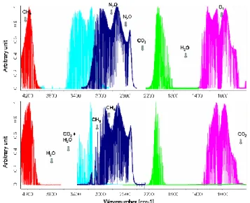
Fig. 1. Composite spectra for different bandpass filters (NDSC-1: red, NDSC-2: blue, NDSC-3: dark blue, NDSC-5: green, and NDSC-6: pink), taken at Ma¨ıdo (upper plot) and at St.-Denis (bottom plot) in 2002, for solar zenith angles between 40 and 50◦.
the target species O3, CH4, N2O, CO, C2H6, HCl, HF and HNO3. Figure 1 shows composite spectra from the first cam-paign in 2002, at Ma¨ıdo and at St.-Denis, including the dif-ferent optical bandpasses (shown in difdif-ferent colours). For this figure, we selected spectra that were recorded on corre-sponding days for both locations and at solar zenith angles between 40 and 50◦. All spectra have been standardized to improve the visibility of the figure. Note that some of the main absorbers are marked. One clearly observes the re-duced absorptions by water vapour at the high-altitude site Ma¨ıdo. For example, the spectral range between 3000 and 3550 cm−1, that is completely opaque at St.-Denis, can be exploited at Ma¨ıdo.
Whenever the sky was clear at local noon, a reference HBr cell spectrum was recorded using the NDSC-4 filter. For this purpose, a cell containing hydrogen bromide (HBr) at low pressure (2 mbar) was placed in the interferometer out-put beam in front of the InSb detector, and a spectrum was recorded using the sun as light source. When this was not possible on several consecutive days because of the noon-time weather situation, the reference HBr cell spectrum was taken the same way, but using a tungsten lamp source. The cell spectra have been analysed using Linefit version 8 (Hase et al., 1999), to monitor the alignment of the instrument. For the ULB instrument at St.-Denis, a cell spectrum was taken only once during the first campaign; it confirmed the correct alignment of the instrument.
Because reliable solar absorption measurements require clear sky conditions, the number of observation days was limited: in total, we had about 24 days with observations dur-ing the first campaign and about 60 days durdur-ing the second
campaign. Also, during the first campaign, it was often not possible to perform the measurements simultaneously at both sites, because the local weather conditions were not necessarily the same. It is worth mentioning that most of the measurements have been carried out before noon, because most often clouds appeared in the afternoon. Sometimes additional late evening measurements have been possible at Ma¨ıdo.
3 General description of the retrieval method
As already mentioned, we have focused on the retrieval of ozone (O3), methane (CH4), nitrous oxide (N2O), carbon monoxide (CO), ethane (C2H6), hydrogen chloride (HCl), hydrogen fluoride (HF) and nitric acid (HNO3). In addi-tion to the total column abundances of these molecules, we have extracted information – whenever feasible – about their vertical distribution in the altitude range where the pressure broadening of the absorption lines can be resolved.
For these retrievals, we have used the inversion algo-rithm SFIT2 (v3.92), jointly developed at the NASA Lan-gley Research Center, the National Center for Atmospheric Research (NCAR) and the National Institute of Water and At-mosphere Research (NIWA) at Lauder, New Zealand (Rins-land et al., 1998). This algorithm uses a semi-empirical im-plementation of the Optimal Estimation Method (OEM) of Rodgers (2000). Further details on the SFIT2 program can be found in the paper by Hase et al. (2004).
All retrievals are executed on a 44 layer altitude grid, starting at 50 m a.s.l. for St.-Denis and at 2200 m a.s.l. for Ma¨ıdo, with layer thicknesses of about 1.2 km in the tropo-sphere and lower stratotropo-sphere up to 33.4 km altitude, then growing steadily to about 4 km around 50 km altitude and to about 8 km for the higher atmospheric layers up to 100 km. This choice was made to take into account the local atmo-spheric pressure and temperature variabilities. Daily pres-sure and temperature profiles were taken from the National Centre for Environmental Prediction (NCEP).
For the error analysis (see Sect. 5.1.4) we also used tem-perature profiles from the European Center for Medium range Weather Forecasting (ECMWF).
3.1 Forward model parameters
The forward model in SFIT2 is a multi-layer multi-species line-by-line radiative transfer model. The instrument param-eters in the forward model include a wavenumber scale mul-tiplier and background curve parameters, as well as the ac-tual optical path difference (OPD) and field of view (FOV) of the instrument. The background slope and curvature are determined by fitting a polynomial of degree 2, and the wave-length shift is also fitted in every spectral micro-window in-dependently.
To account for deviations from the ideal instrument line shape function (ILS) due to small instrument misalignments or imperfections, apodization and phase error functions are included. These functions can either be acquired from the Linefit analyses of the measured HBr cell spectra, or they can be approximated by a polynomial or a Fourier series of a user specified order. Our retrievals have been carried out using the second approach, i.e., fitted empirical apodization and phase error functions, because in all our retrievals this approach resulted in the smallest spectral residuals and the least oscillations in the retrieved profiles. In particular, we approximated the empirical apodization by a polynomial of degree 2 and, if beneficial, the empirical phase error by a polynomial of degree 1.
3.2 Inverse model
The inverse problem consists of determining the state of the atmosphere, in particular the vertical distributions of the tar-get molecules, from the observed absorption spectra. In order to solve this ill-posed problem, the SFIT2 retrievals request ad hoc covariance matrices for the uncertainties associated with the a priori vertical profiles of the target gases and with the measurements. The retrieved profiles and total column amounts of the target species are the ones that provide the best representation of the truth, given the measurements and the a priori information, and their respective uncertainties.
3.2.1 A priori profile and associated covariance matrix
The used a priori profile xa and its covariance matrix Sa should well represent a first guess of the ‘true’ state, in order to reasonably constrain the retrieval solution, in particular at those altitudes where one can hardly get information out of the measurements. For each target gas we have decided to use one single a priori profile and associated covariance matrix for both campaigns, to avoid any biases between the results and to make sure that the results are directly compa-rable. The diagonal and off-diagonal elements of each Sa have been chosen such as to yield the best compromise be-tween the spectral residuals, the number of oscillations in the retrieved profiles, and the number of degrees of freedom for signal (DOFS; see Sect. 3.3). We have assumed that the cor-relations between the layers decay according to a Gaussian-shaped function. Details about the choice of the a priori ver-tical profiles and the associated covariance matrices are pro-vided for each molecule individually in Sect. 4.2.
While we used constant values on the diagonal of Sa for the retrievals of all molecules, except CH4, we used more re-alistic uncertainties in the error calculations. Nevertheless, the Sa matrices used in the error analysis still have a Gaus-sian shape because of the limited knowledge about their full structure.
3.2.3 Selection of spectral micro-windows
Deriving information about the vertical distribution of trace gases out of high resolution FTIR spectra is possible because of the pressure broadening of the absorption lines, leading to an altitude dependence of the line shapes. While the line centers provide information about the higher altitudes of the distribution, the wings of a line provide information about the lower altitudes. Therefore the information content of the retrieval will strongly depend on the choice of the absorption lines. For all species, the absorption line parameters were taken from the HITRAN 2004 spectral database (Rothman et al., 2005). In addition, updates for H2O, N2O, HNO3 and C2H6line parameters that are available on the HITRAN site (http://www.hitran.com) have been included. We have veri-fied that they give similar or slightly better spectral fits than the original HITRAN 2004 values.
The retrieval spectral micro-windows are selected such that they contain unsaturated well-isolated absorption fea-tures of the target species with a minimal number of inter-fering absorption lines. One also aims at maximizing the amount of information present in the spectra, represented by the DOFS.
For the present retrievals, we adopted spectral micro-windows used by other FTIR research groups and we veri-fied slight modifications of those micro-windows, in order to improve our retrievals.
Further details about the micro-window selections and characteristics are discussed in Sect. 4.1.
3.3 Information content and sensitivity
The retrieved state vector xr is related to the a priori and the true state vectors xaand x, respectively, by the equation
xr =xa+ A (x − xa) (1)
(Rodgers, 2000).
The rows of the matrix A are called the averaging kernels and the trace of A equals the DOFS. For each of the 44 lay-ers the full width at half maximum of the averaging kernels provides an estimate of the vertical resolution of the profile retrieval at the corresponding altitude, while the area of the averaging kernel represents the sensitivity of the retrieval at the corresponding altitude to the true state. The DOFS to-gether with the averaging kernel shapes will define the
par-windows (fitted simultaneously), the spectral resolution, the effective SNR, and the associated interfering molecules, to-gether with our choice of the diagonal elements and the half-widths at half-maximum (HWHM) defining the Gaussian inter-layer correlation length of Saadopted in the retrieval, and finally also the achieved mean DOFS for each target species, at Ma¨ıdo in 2002, and at St.-Denis in 2002 and 2004. 4.1 Spectral micro-window selections
The micro-windows in which O3, CH4, N2O, CO and C2H6 are retrieved, as well as the interfering absorbers whose to-tal columns are fitted simultaneously with the target species, have been adopted from the EC project UFTIR (http://www. nilu.no/uftir; De Mazi`ere et al., 2004). Our tests have shown that these windows are still appropriate for the Ma¨ıdo and St.-Denis sites at Ile de La R´eunion, despite the prevailing high humidity.
The UFTIR project also provided us with corrected spec-tral line parameters for ozone in the 2960–2980 cm−1region (D. Mondelain and A. Barbe, private communication), which improve the spectral fits for C2H6. For HF and HCl the fitted micro-windows and interfering species were adopted from Reisinger et al. (1994) and from Rinsland et al. (2003), respectively. For the HCl retrievals, Rinsland et al. (2003) propose to fit two other micro-windows around 2727.78 and 2775.78 cm−1, in addition to the two windows we use. But since they contain strong interfering water vapour lines, fit-ting them appeared to be problematic at our (sub)tropical site. We therefore restricted our spectral fits to the two micro-windows defined in Table 1. The HNO3 micro-window se-lection is based on the discussions by Flaud et al. (2006) and Perrin et al. (2004).
4.2 Construction of a priori information and retrieval re-sults
4.2.1 Ozone (O3)
For the O3 retrievals, we adopted a single mean a priori profile from the UGAMP (UK Universities Global Atmospheric Modelling Programme, http://ugamp. nerc.ac.uk/) climatology, calculated for a square of 2.5◦×2.5◦ enclosing St.-Denis (http://badc.nerc.ac.uk/data/ ugamp-o3-climatology/), which provides a global 4-D
Table 1. Summary of the retrieval characteristics for each target species, for the FTIR campaigns at Ile de La R´eunion. Variab. represents the diagonal elements of Saand HWHM the inter-layer correlation length in SaThe fourth, fifth and seventh columns list the spectral micro-windows that are fitted simultaneously, the associated spectral resolution, and the main interfering species. SNR is the ad hoc signal-to-noise ratio adopted in the retrievals. The last column provides the mean DOFS achieved at Ma¨ıdo, 2002, and at St.-Denis, 2002 and 2004.
Molecule Variab. [%] HWHM Micro-window(s) Spectral resolution SNR Interfering DOFS Ma¨ıdo /
[km] [cm−1] [cm−1] species St.-Denis O3 20 6 1000.00–1005.00 0.0072 150 H2O 4.9 / 5.1 CH4 variable 5 2613.70–2615.40 0.00513 250 HDO, H2O 2.2 / 2.4 2650.60–2651.30 (fitted first), 2835.50–2835.80 CO2 2903.60–2904.03 2921.00–2921.60 N2O 10 5 2481.30–2482.60 0.00513 150 CO2, CH4, O3, 3.0 / 3.2 2526.40–2528.20 H2O, HDO 2537.85–2538.80 2540.10–2540.70 CO 20 4 2057.70–2057.91 0.0036 150 O3, OCS, CO2, 2.6 / 2.8 2069.55–2069.72 N2O, H2O, 2157.40–2159.35 solar CO lines C2H6 40 5 2976.50–2977.20 0.00513 250 H2O, CH4, O3 1.5 / 1.7 HCl 20 5 2843.30–2843.80 0.00513 150 H2O, CH4, HDO 1.2 / 1.4 2925.70–2926.60 HF 20 3 4038.70–4039.05 0.0072 300 H2O 1.4 / 1.5 HNO3 20 5 872.25–874.80 0.01098 200 OCS, C2H6, H2O 1.0 / 1.2
climatological distribution of ozone covering the years 1985 to 1989 and the altitude range 0 to 100 km.
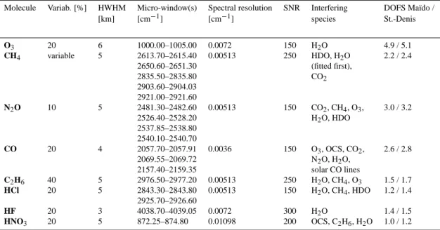
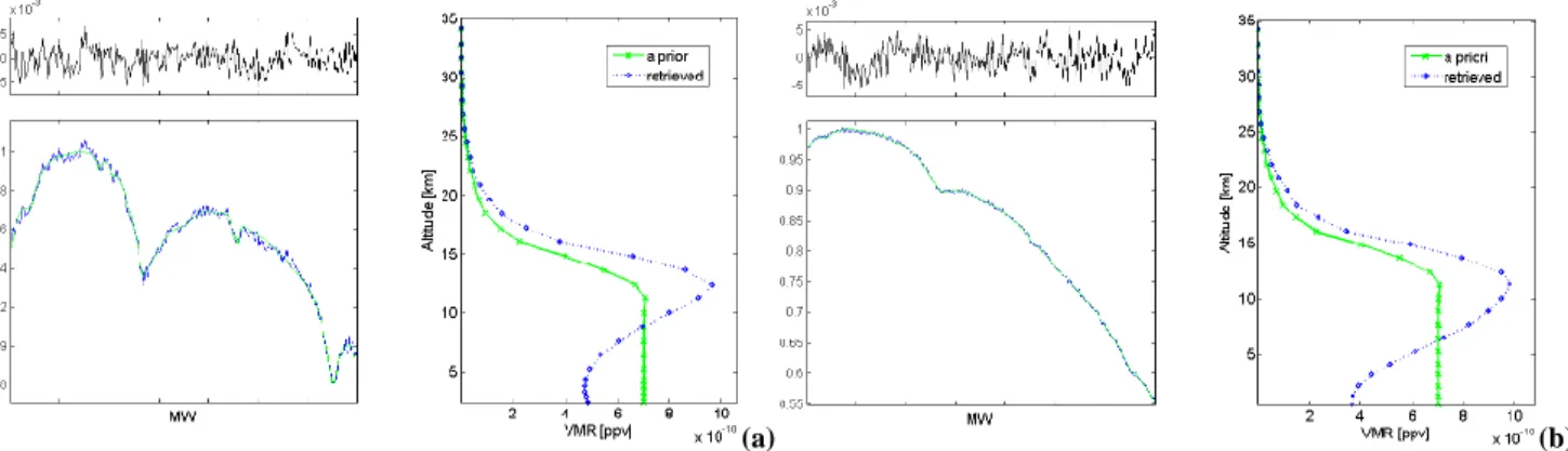
Figure 2 shows the single micro-window fit of O3 from a single spectrum on 13 October 2002 and 15 October 2004 at Ma¨ıdo and St.-Denis, respectively, together with the residuals, computed as measured minus simulated transmis-sion. In the spectral fits for St.-Denis we observe systematic residuals around 1001.10 and 1003.70 cm−1, which are due to water vapour lines. However, fitting H2O profiles first to use the resulting daily a priori profiles in the O3retrieval, or excluding the two small regions from our micro-window, did not affect the retrievals significantly.
We obtain about 5 degrees of freedom for O3at both sites. It is therefore possible to distinguish 5 independent layers with good sensitivity, namely 2 layers in the troposphere (2.2 / 0.1 to 8.2 and 8.2 to 17.8 km), and 3 layers in the strato-sphere (17.8 to 23.8, 23.8 to 31.0 and 31.0 to 100 km). 4.2.2 Methane (CH4)
The CH4 a priori profile was based on available data from the Halogen Occultation Experiment (HALOE), onboard the Upper Atmosphere Research Satellite (UARS), launched in September 1991 (http://haloedata.larc.nasa.gov/home). CH4 retrievals from HALOE have been validated by Park et al. (1996). We took a six year weighted mean of all HALOE (version 19) vertical profiles from 2000 to 2005 within the 15◦ longitude and 10◦ latitude rectangle around Ile de La
R´eunion, with weights defined by the errors that are provided together with the HALOE profiles.
The resulting weighted mean profile covers the range 14 to 80 km, so below and above these altitudes we have extrapolated the profile by repeating the values at 14 and 80 km, respectively. In contrast to all other retrieved molecules we have used non constant diagonal elements to construct Sa. This is done, because it significantly reduces the large oscillations in the retrieved profiles that emerge when using constant uncertainties. The values are calculated out of the same HALOE profiles as used to determine the a priori profile. The obtained variabilities (in percentage) from 14.2 to 78.4 km are then extrapolated to the complete altitude range by repeating the first and last value. The off-diagonal elements are defined by a Gaussian distribution hav-ing a HWHM of 5 km and finally the matrix is transformed into squared volume mixing ratio units.
Figure 3 shows the multiple micro-window fit of CH4from a single spectrum on 16 October 2002 and 12 October 2004 at Ma¨ıdo and St.-Denis, respectively, together with the resid-uals, computed as measured minus simulated transmission. Note that the retrieved profiles slightly oscillate near the sur-face.
As the number of degrees of freedom is about 2 at both sites, we manage to resolve two independent partial columns of CH4, namely 2.2 to 11.8 km and 11.8 to 100 km for Ma¨ıdo and 0.1 to 8.2 and 8.2 to 100 km for St.-Denis.
(a) (b) Fig. 2. Single micro-window (1000.00–1005.00 cm−1)fit of O3plus interfering species from a single spectrum on (a) 13 October 2002 at Ma¨ıdo and on (b) 15 October 2004 at St.-Denis. Measured (blue) and simulated spectra (green) are shown (left lower plot), together with the residuals (left upper plot), computed as measured minus simulated. The right plot shows the a priori (green crosses) and retrieved (blue diamonds) profile.
(a) (b)
Fig. 3. Multiple micro-window (MW1: 2613.70–2615.40, MW2: 2650.60–2651.30, MW3: 2835.50–2835.80, MW4: 2903.60–2904.03, and MW5: 2921.00–2921.60 cm−1)fit of CH4plus interfering species from a single spectrum on (a) 16 October 2002 at Ma¨ıdo and on (b) 12 October 2004 at St.-Denis. Measured (blue) and simulated spectra (green) are shown (left lower plot), together with the residuals (left upper plot), computed as measured minus simulated. The right plot shows the a priori (green crosses) and retrieved (blue diamonds) profile.
4.2.3 Nitrous oxide (N2O)
For the N2O a priori profile we used the 1976 U.S. Standard profile (U.S. NOAA, 1976) scaled with a yearly factor of 0.25%, to account for the slight yearly N2O increase ob-served by Zander et al. (2005).
Figure 4 shows the multiple micro-window fit of N2O from a single spectrum on 16 October 2002 and 12 October 2004 at Ma¨ıdo and St.-Denis, respectively, together with the residuals, computed as measured minus simulated transmis-sion.
As the number of degrees of freedom for N2O is about 3 for Ma¨ıdo as well as for St.-Denis, three independent partial columns can be distinguished, in particular from 2.2 / 0.1 to 4.6, from 4.6 to 15.4 and from 15.4 to 100 km.
4.2.4 Carbon monoxide (CO)
The CO a priori profile has been based on available data from the MOPITT space-borne instrument onboard the EOS-TERRA satellite, which was launched in December 1999 (http://terra.nasa.gov/About/MOPITT/index.php). CO retrievals from MOPITT have been validated by Emmons et al. (2004). Our CO a priori profile is a five year mean of all MOPITT vertical profiles (version L2V5) from 2000 to 2004 within 15◦longitude and 10◦latitude around the loca-tion of our observaloca-tions. We only used daytime measure-ments for which the solar zenith angle was smaller than 80◦. The thus obtained mean a priori profile from 0 to 14 km was then completed with the U.S. Standard Atmosphere (1976) values from 16 to 100 km.
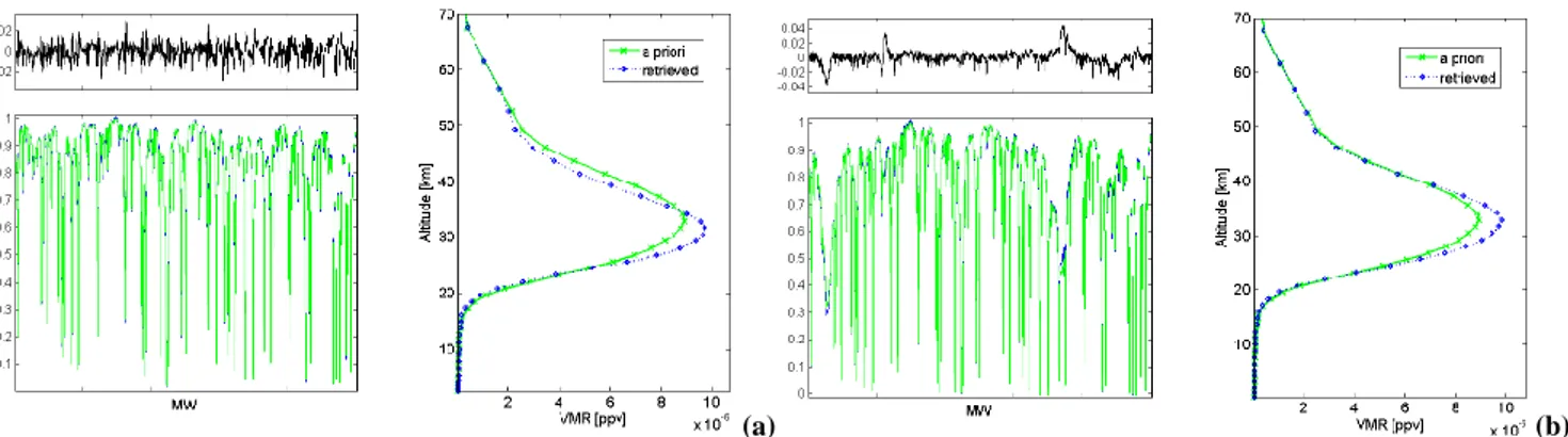
Figure 5 shows the multiple micro-window fit of CO from a single spectrum on 19 October 2002 and 12 October 2004 at Ma¨ıdo and St.-Denis, respectively, together with the resid-uals, computed as measured minus simulated transmission.
(a) (b) Fig. 4. Multiple micro-window (MW1: 2481.30–2482.60, MW2: 2526.40–2528.20, MW3: 2537.85–2538.80, and MW4: 2540.10– 2540.70 cm−1)fit of N2O plus interfering species from a single spectrum on (a) 16 October 2002 at Ma¨ıdo and on (b) 12 October 2004 at St.-Denis. Measured (blue) and simulated spectra (green) are shown (left lower plot), together with the residuals (left upper plot), computed as measured minus simulated. The right plot shows the a priori (green crosses) and retrieved (blue diamonds) profile.
(a) (b)
Fig. 5. Multiple micro-window (MW1: 2057.70–2057.91, MW2: 2069.55–2069.72, and MW3: 2157.40–2159.35 cm−1)fit of CO plus interfering species from a single spectrum on (a) 19 October 2002 at Ma¨ıdo and on (b) 12 October 2004 at St.-Denis. Measured (blue) and simulated spectra (green) are shown (left lower plot), together with the residuals (left upper plot), computed as measured minus simulated. The right plot shows the a priori (green crosses) and retrieved (blue diamonds) profile.
From the first figure it is clear that for the 2002 spectra the CO micro-windows are contaminated by noise, due to the bad filters choice.
The DOFS for CO in our measurements is about 2.7, providing us with just 2 independent layers, namely 2.2 to 10.6 km and 10.6 to 100 km for Ma¨ıdo and 0.1 to 9.4 and 9.4 to 100 km for St.-Denis.
4.2.5 Ethane (C2H6)
Between 12 and 30 km, the a priori profile for C2H6 was adopted from Cronn and Robinson (1979) and above 30 km from Rudolph and Ehhalt (1981). Below 12 km the a priori volume mixing ratio was set constant at 7×10⁻¹⁰ppv.
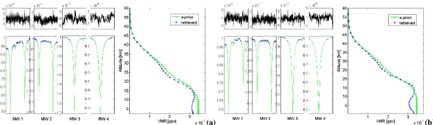
Figure 6 shows the single micro-window fit of C2H6from a single spectrum on 14 October 2002 and 9 October 2004 at Ma¨ıdo and St.-Denis, respectively, together with the residu-als, computed as measured minus simulated.
Since we obtain about 1.6 degrees of freedom, we consider only total column amounts of C2H6.
4.2.6 Hydrogen chloride (HCl)
The HCl a priori profile between 16 and 60 km was created from HALOE (version 19) observations, following the same approach as for CH4. HCl retrievals from HALOE have been validated by Russell et al. (1996a). Below 16 km the pro-file was completed with values from Smith (1982) and above 60 km a constant mixing ratio was adopted, which was equal to the upper value of the weighted mean HALOE profile.
Figure 7 shows the multiple micro-window fit of HCl from a single spectrum on 16 October 2002 and 15 October 2004 at Ma¨ıdo and St.-Denis, respectively, together with the resid-uals, computed as measured minus simulated transmission. Note that around 25 km the retrieved profile differs strongly from the a priori profile. Such deviations are observed for all our HCl measurements, but up to now we did not manage to find the origin of this structure.
Again, we can only derive total column amounts, because the number of degrees of freedom for HCl is about 1.3 at both sites.
(a) (b) Fig. 6. Single micro-window (2976.50–2977.20 cm−1)fit of C2H6plus interfering species from a single spectrum on (a) 14 October 2002 at Ma¨ıdo and on (b) 9 October 2004 at St.-Denis. Measured (blue) and simulated spectra (green) are shown (left lower plot), together with the residuals (left upper plot), computed as measured minus simulated. The right plot shows the a priori (green crosses) and retrieved (blue diamonds) profile.
(a) (b)
Fig. 7. Multiple micro-window (MW1: 2843.30–2843.80 and MW2: 2925.70–2926.60 cm−1)fit of HCl plus interfering species from a single spectrum on (a) 16 October 2002 at Ma¨ıdo and on (b) 15 October 2004 at St.-Denis. Measured (blue) and simulated spectra (green) are shown (left lower plot), together with the residuals (left upper plot), computed as measured minus simulated. The right plot shows the a priori (green crosses) and retrieved (blue diamonds) profile.
4.2.7 Hydrogen fluoride (HF)
The HF a priori profile between 14 and 60 km was derived from HALOE (version 19) observations, as was done for HCl. HF retrievals from HALOE have been validated by Russell et al. (1996b). The profile was extrapolated with con-stant values above and below that altitude range, by repeating the volume mixing ratio at 60 and 14 km, respectively.
Figure 8 shows the single micro-window fit of HF from a single spectrum on 13 October 2002 and 11 October 2004 at Ma¨ıdo and St.-Denis, respectively, together with the residu-als, computed as measured minus simulated transmission.
The 1.5 degrees of freedom tell us that we can only deter-mine the total columns of HF.
4.2.8 Nitric acid (HNO3)
For the creation of an HNO3 reference profile, we used data from the SMR instrument, onboard the satellite Odin, launched in February 2001 (http://diamond.rss.chalmers.se/
Odin). HNO3retrievals from Odin have been validated by Urban et al. (2005). In particular, we calculated a five year weighted mean, from 2001 to 2005, of all Odin/SMR profiles (version 2.0) within a 1500 km radius around St.-Denis, with weights defined by the errors on the Odin profiles. This gave us representative a priori values between 16 and 36 km. Be-low and above these altitudes we completed the profile with a seasonal mean climatology for the 0◦–20◦S latitude band in the period September–November 2002 from the Michelson Interferometer for Passive Atmospheric Sounding (MIPAS) onboard ESA’s Envisat satellite, launched in March 2002 (http://envisat.esa.int/instruments/mipas/index.html). HNO3 retrievals from MIPAS have been validated by Oelhaf et al. (2004) and Wang et al. (2007).
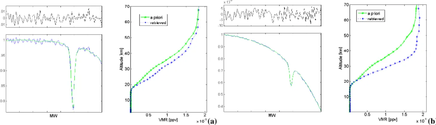
Figure 9 shows the single micro-window fit of HNO3from a single spectrum on 16 October 2002 and 21 October 2004 at Ma¨ıdo and St.-Denis, respectively, together with the resid-uals, computed as measured minus simulated transmission.
For HNO3we get about 1 degree of freedom, so again only total column amounts can be obtained.
(a) (b) Fig. 8. Single micro-window (4038.70–4039.05 cm−1)fit of HF plus interfering species from a single spectrum on (a) 13 October 2002 at Ma¨ıdo and on (b) 11 October 2004 at St.-Denis. Measured (blue) and simulated spectra (green) are shown (left lower plot), together with the residuals (left upper plot), computed as measured minus simulated. The right plot shows the a priori (green crosses) and retrieved (blue diamonds) profile.
(a) (b)
Fig. 9. Single micro-window (872.25–874.80 cm−1)fit of HNO3plus interfering species from a single spectrum on (a) 16 October 2002 at Ma¨ıdo and on (b) 21 October 2004 at St.-Denis. Measured (blue) and simulated spectra (green) are shown (left lower plot), together with the residuals (left upper plot), computed as measured minus simulated. The right plot shows the a priori (green crosses) and retrieved (blue diamonds) profile.
5 Error budget evaluations
5.1 Adopted approach
Using the formalism described in Rodgers (2000) – assuming a linearization of the forward and inverse model about some reference state and spectrum, respectively – the difference between the retrieved and the real state of the atmosphere can be written as
xr−x = (A − I) (x − xa) +GyKb(b − br) +Gy(y − yr),(2) where A is the averaging kernel matrix as defined in Sect. 3.3,
I the identity matrix, Gythe gain matrix representing the sen-sitivity of the retrieved parameters to the measurement, Kb the sensitivity matrix of the spectrum to the forward model parameters b, br the estimated model parameters, y the ob-served spectrum, and yr the calculated spectrum correspond-ing to the retrieved state vector. The equation above splits the total error in the retrieved profile into three different error
sources, i.e., the smoothing error, the forward model param-eter error and the measurement error. In addition, we have determined the temperature and interfering species error as individual contributions to the total random error. Besides the random errors we must also consider the systematic er-rors due to uncertainties in the spectroscopic line parameters. More details about the evaluation of the individual contribu-tions to the error budget are provided in the next seccontribu-tions. 5.1.1 Smoothing error
The smoothing error covariance is calculated as (I−A) Sa (I−A)t, where Sa is the a priori covariance matrix (see Sect. 3.2.1). In order to construct a realistic Sa matrix, we need information about the variability and covariances of an ensemble of real profiles. However, this information is not al-ways available at all altitudes, obliging us to replace Sawith a Gaussian covariance matrix for example, for which we still have to estimate the natural variabilities and the inter-layer
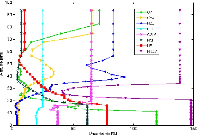
Fig. 10. A priori uncertainties (in %) in the volume mixing ratios of each retrieved trace gas as a function of altitude, used for estimating the smoothing errors.
correlations based on real data. We have chosen these values such that Sa approaches the covariance matrix derived from satellite measurements within the available altitude range. For each species we calculated the weighted covariance ma-trix of all available vertical profiles measured by the specified satellite within the 15◦longitude and 10◦latitude rectangle around Ile de La R´eunion, and used the resulting diagonal elements to create Sa. The thus obtained variabilities that are reliable within a certain altitude range are then extrapolated to the complete altitude range (0–100 km) by repeating the lower- and uppermost values in percentage. The off-diagonal elements of Sa are defined by a Gaussian distribution hav-ing a HWHM which can be different for each molecule. The resulting matrix is then transformed into squared vol-ume mixing ratio units. Table 2 summarizes which satellite data have been used for every trace gas, the altitude range in which they provide reliable values and the HWHM used to calculate the Gaussian off-diagonal elements of the Sa ma-trix. For more information about the satellite data used, we refer to Sect. 6.1. Figure 10 shows the resulting uncertain-ties in the a priori volume mixing ratios of each species as a function of altitude.
5.1.2 Forward model parameter error
We considered the random uncertainties in the forward model parameters, described in Sect. 3.1, to be mutually independent; hence we used a matrix Sb that is diagonal. For the wavenumber shift, background curve parameters, and ILS parameters, we adopted uncertainties of 10%, 10%, and 20%, respectively. The resulting errors on the retrieved target profile are then calculated as (GyKb)Sb(GyKb)t.
C2H6 ACE 10.6–20.2 3
HCl HALOE 15.4–58.8 7
HF HALOE 15.4–64.4 6
HNO3 Odin 20.2–34.8 4
Fig. 11. Temperature covariance matrix (in K2) from NCEP and ECMWF temperature profiles at Ile de La R´eunion in October 2004, used for estimating the temperature errors.
5.1.3 Measurement error
The uncertainties coming from the measurement noise are calculated as GySεGty, where Sε is the measurement noise covariance matrix, defined as a diagonal matrix consisting of the squared noise in the observed spectra. These noise values have been determined for every fitted micro-window inde-pendently, as the root mean squared value (rms) of the differ-ences between the observed and calculated spectrum within each bandpass.
5.1.4 Temperature error
The atmospheric temperature profile is a forward model pa-rameter that is not fitted. Nevertheless, the associated uncer-tainties must be considered as well, because they influence the retrieved profiles via the temperature dependence of the absorption lines. The temperature error covariance matrix is calculated as (GyKT)ST (GyKT)t, in which ST is a realistic covariance matrix of the temperature profile uncertainties.
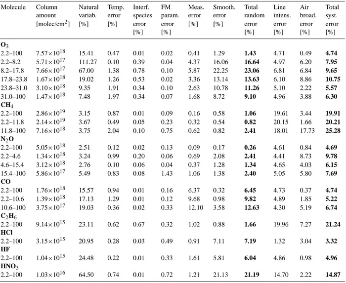
Table 3. Summary of the error budgets (in %) on the total (2.2–100 km) and partial columns (altitude ranges specified in km) for each target species retrieved from the Ile de La R´eunion campaign data, for Ma¨ıdo 2002. The total and partial column amounts (in molecules/cm2) and corresponding natural variabilities (in %) are listed in the second and third columns, respectively.
Molecule Column Natural Temp. Interf. FM Meas. Smooth. Total Line Air Total amount variab. error species param. error error random intens. broad. syst. [molec/cm2] [%] [%] error error [%] [%] error error error error
[%] [%] [%] [%] [%] [%] O3 2.2–100 7.57×10¹⁸ 15.41 0.47 0.01 0.02 0.41 1.29 1.43 4.71 0.49 4.74 2.2–8.2 5.71×10¹⁷ 111.27 0.10 0.39 0.04 4.37 16.06 16.64 4.97 6.20 7.95 8.2–17.8 7.66×10¹⁷ 67.00 1.38 0.78 0.10 5.87 22.25 23.06 6.81 6.84 9.65 17.8–23.8 1.67×10¹⁸ 19.02 1.26 0.53 0.02 3.36 13.14 13.63 6.10 8.86 10.75 23.8–31.0 3.10×10¹⁸ 9.35 1.91 0.34 0.10 2.63 10.78 11.26 5.10 2.22 5.57 31.0–100 1.47×10¹⁸ 7.48 1.97 0.34 0.07 1.68 8.72 9.10 4.96 3.88 6.30 CH4 2.2–100 2.86×10¹⁹ 3.15 0.87 0.01 0.09 0.16 0.58 1.06 19.61 3.44 19.91 2.2–11.8 2.14×10¹⁹ 3.67 0.49 0.05 0.23 0.32 0.54 0.82 20.15 1.66 20.21 11.8–100 7.16×10¹⁸ 3.75 2.04 0.10 0.75 0.62 0.82 2.41 18.01 17.73 25.28 N2O 2.2–100 5.05×10¹⁸ 2.51 0.12 0.02 0.13 0.09 0.17 0.26 4.61 0.84 4.69 2.2–4.6 1.34×10¹⁸ 3.24 0.99 0.20 0.06 0.69 2.08 2.41 4.41 8.73 9.78 4.6–15.4 3.12×10¹⁸ 2.76 0.10 0.06 0.04 0.37 1.28 1.34 4.65 4.03 6.15 15.4–100 5.86×10¹⁷ 5.49 0.83 0.08 1.43 1.06 1.38 2.40 5.05 5.80 7.69 CO 2.2–100 1.76×10¹⁸ 15.57 0.94 0.01 0.16 6.37 0.32 6.45 4.73 0.37 4.74 2.2–10.6 1.39×10¹⁸ 17.13 1.29 0.01 0.12 9.68 0.98 9.82 4.89 1.85 5.22 10.6–100 3.75×10¹⁷ 19.03 0.36 0.02 0.33 12.10 3.58 12.63 4.30 5.19 6.74 C2H6 2.2–100 9.14×10¹⁵ 23.11 0.62 0.67 0.32 1.02 0.88 1.66 19.96 7.27 21.24 HCl 2.2–100 3.15×10¹⁵ 20.95 0.28 0.03 0.49 0.91 7.11 7.19 1.32 3.04 3.32 HF 2.2–100 1.04×10¹⁵ 24.48 0.22 0.01 0.33 1.61 5.81 6.04 4.86 0.98 4.96 HNO3 2.2–100 1.03×10¹⁶ 64.50 0.74 0.01 0.72 1.21 21.13 21.19 14.70 2.22 14.87
The factor (GyKT), containing the partial derivatives of the retrieval to the temperatures, has been determined by repeating the retrieval with temperature profiles that are slightly perturbed at all altitudes separately. Our estimation of ST is based on the differences between the NCEP and ECMWF temperature profiles for Ile de La R´eunion in the period August–October 2004. Its elements are calculated as
ST(i, j) = E[(TNCEP(i) −TECMWF(i)) ∗
(TNCEP(j ) −TECMWF(j ))]. (3) This matrix is visualized in Fig. 11. The 41 profile layers from high to low altitude are defined as follows: from 100 to 50 km by steps of 5 km, from 50 to 10 km by steps of 2 km and from 10 km to the surface by steps of 1 km. As the NCEP profiles do not reach higher than about 54 km, we have re-peated the covariances at 50 km for all altitudes above.
5.1.5 Interfering species error
The error on the retrieval of a target gas coming from the uncertainties in the vertical distributions of the interfering species has been calculated by performing retrievals using an ensemble of vertical profiles of every significant interferer separately, representing the uncertainties in its a priori profile (Sussmann and Borsdorff, 2007; Connor et al., 2008). Con-sequently we derive an error covariance matrix based on the thus obtained set of retrieved target profile differences rela-tive to the reference profile, which represents the contribution of the interfering species uncertainties to the random error.
We have observed that when considering only the total column uncertainties of the interfering species, this error component is clearly underestimated in some cases.
0.05–100 7.78×10 14.43 0.50 0.12 0.01 0.31 0.57 0.82 4.68 0.38 4.69 0.05–8.2 6.46×10¹⁷ 106.23 0.09 1.02 0.02 3.84 10.71 11.42 5.60 4.51 7.19 8.2–17.8 6.80×10¹⁷ 61.72 1.86 1.38 0.09 4.75 13.53 14.53 5.04 4.68 6.87 17.8–23.8 1.82×10¹⁸ 19.38 1.59 1.65 0.04 3.23 8.88 9.73 5.20 7.49 9.12 23.8–31.0 3.05×10¹⁸ 9.31 2.37 1.48 0.10 2.50 5.97 7.05 4.31 1.74 4.65 31.0–100 1.59×10¹⁸ 7.32 1.89 0.92 0.10 2.39 6.60 7.33 5.18 3.91 6.49 CH4 0.05–100 3.58×10¹⁹ 3.06 1.08 0.48 0.01 0.25 0.18 1.22 19.94 3.17 20.19 0.05–8.2 2.23×10¹⁹ 3.78 1.17 0.76 0.21 0.70 0.58 1.68 20.69 6.19 21.60 8.2–100 1.35×10¹⁹ 3.43 0.94 0.94 0.39 0.68 0.60 1.66 18.69 18.49 26.29 N2O 0.05–100 6.63×10¹⁸ 2.44 0.18 0.02 0.09 0.08 0.15 0.27 4.59 0.79 4.66 0.05–4.6 2.89×10¹⁸ 3.17 0.80 0.16 0.14 0.32 0.89 1.25 4.64 6.88 8.30 4.6–15.4 3.11×10¹⁸ 2.75 0.34 0.13 0.14 0.25 0.91 1.02 4.62 7.17 8.53 15.4–100 6.26×10¹⁷ 5.34 0.20 0.13 1.04 0.53 1.20 1.69 4.36 4.82 6.50 CO 0.05–100 2.96×10¹⁸ 14.95 0.69 0.05 0.17 0.46 0.37 0.93 3.05 0.16 3.06 0.05–9.4 2.32×10¹⁸ 16.80 0.73 0.04 0.14 0.65 1.06 1.45 2.92 1.02 3.09 9.4–100 6.38×10¹⁷ 18.51 0.54 0.15 0.38 2.09 3.79 4.38 3.57 2.97 4.65 C2H6 0.05–100 1.20×10¹⁶ 22.46 0.78 2.16 0.72 1.92 1.47 3.41 14.67 3.04 14.98 HCl 0.05–100 3.16×10¹⁵ 22.63 0.17 0.67 0.41 2.27 10.95 11.21 2.50 4.00 4.72 HF 0.05–100 1.32×10¹⁵ 26.51 0.15 0.12 0.19 1.96 13.57 13.71 3.53 0.20 3.54 HNO3 0.05–100 9.58×10¹⁵ 60.40 1.28 0.27 0.87 2.71 25.61 25.80 33.32 7.00 34.05
5.1.6 Line intensity and pressure broadening error
In addition to the random error budget, we determined the systematic error in the retrievals originating from the un-certainties in the spectroscopic line intensities and in the pressure broadening coefficients. We therefore performed retrievals with perturbed spectroscopic line intensities and broadening coefficients of the target lines within our micro-windows. The perturbation of these line parameters is based on their maximum uncertainties as given by Rothman et al. (2005). While for all molecules, except for CH4 and HNO3, these uncertainties are specified within certain limits, for CH4and HNO3we assumed the uncertainties on the line intensities to be 20 and 25%, respectively, as they are only specified to be larger than or equal to 20%. The correspond-ing systematic error covariance matrices are then calculated
based on the differences between the thus retrieved vertical profiles and the originally retrieved profiles.
5.2 Discussion
The estimated error values for representative Ma¨ıdo and St.-Denis spectra, recorded at solar zenith angles between 40 and 65◦, are summarized in Table 3 and Table 4, respectively. Note that we only show the error values for the 2004 cam-paign at St.-Denis, because the 2002 camcam-paign at this loca-tion yields similar values.
The systematic errors are generally dominated by the un-certainties in the line intensities. For all species, they are very similar at both locations. This is a logical consequence of the fact that we use the same spectroscopic database and the same retrieval strategy for both sites.
In particular, the systematic errors are especially high for CH4, HNO3 and C2H6, because of strong uncertainties in their spectroscopic line parameters.
It can also be seen in Tables 3 and 4 that the uncertainties on the air broadening coefficients significantly affect the er-rors on the profile retrieval, or the partial column erer-rors, but that they have a smaller impact on the total column errors, as one might expect. Only in the case of HCl, the error on the total column due to air broadening coefficient uncertainties is larger than the one due to line intensity uncertainties.
Regarding the total column smoothing error, we observe that it is larger for the stratospheric species than for the tro-pospheric species, at both sites. Generally it becomes larger with decreasing DOFS, and when the true profile has more vertical structure. For most molecules, we see slightly larger PC smoothing errors at Ma¨ıdo, where the DOFS is slightly smaller. If the DOFS exceeds one, the smoothing error is larger for the independent partial columns than it is for the total column. The smoothing error is highest for the par-tial columns in which the species’ profile has more vertical structure. For the stratospheric species, the smoothing error is the dominant contribution to the random error. For the other species, the main error source may vary.
Only in the case of CO and C2H6at Ma¨ıdo the measure-ment noise is the dominant random error contribution. C2H6 is a very weak signature, making the SNR very small. As to CO, we remind the reader (see Sect. 2) that in 2002 at Ma¨ıdo, we made a less appropriate choice of optical filter and de-tector for the observation of the spectral range in which the CO micro-windows are located, causing a lower SNR and therefore a larger measurement error. The measurement error listed in Table 4 for CO at St.-Denis represents the nominal case.
The temperature error is more important when the lower state energies of the absorbing lines in the micro-windows become higher, which is the case for example for some CH4 and O3lines. It is quite similar at Ma¨ıdo and St.-Denis.
The error due to interfering species uncertainties is dominated by the uncertainties on the HDO and H2O pro-files. That explains why it is an important error source for species with strong H2O and/or HDO interfering lines, like O3, CH4, HCl and C2H6. As all other interfering species un-certainties have a negligible impact on the target species, we only included the error budgets due to uncertainties on H2O and/or HDO in Tables 3 and 4.
We see that in all cases this error is larger at the near sea level site St.-Denis than at the high-altitude site Ma¨ıdo, con-firming the fact that the mountain site is much less affected by the high humidity in the (sub)tropics. Actually the mean H2O column amount observed above Ma¨ıdo during our first campaign is about 1.5×10²²molecules/cm2, while above St.-Denis it is about 7×10²²molecules/cm2, respectively! The interfering species error on the total columns is below 0.7% for all cases at Ma¨ıdo, whereas it rises to about 2.2% for C2H6at St.-Denis.
The forward model parameter error never is the dominant error source, except for the partial column of N2O above Ma¨ıdo, above 15.4 km. This error source is similar at both measurement stations.
It is important to note that in all cases the total random er-rors are smaller than the species’ natural variability, except for the upper two partial columns of O3at Ma¨ıdo. This im-plies that we can effectively extract useful information from the obtained partial and total column time series.
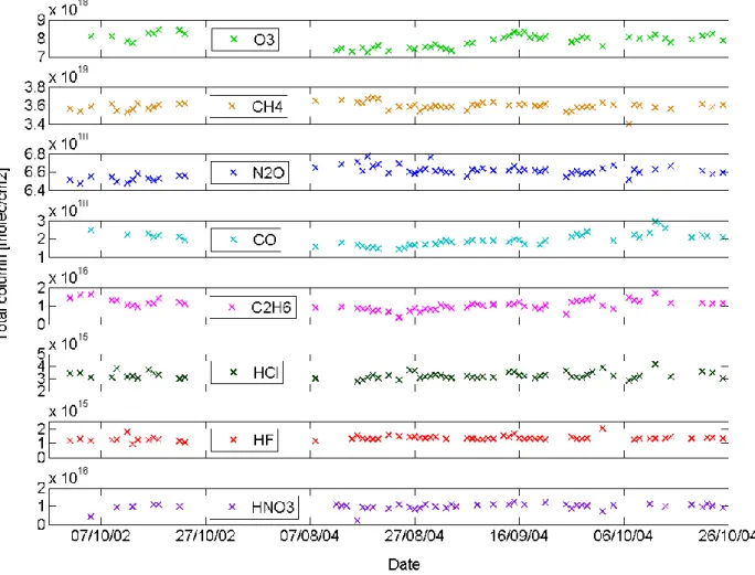
6 Discussion of the retrieval results and comparison with correlative data
Figure 12 shows the time series of the retrieved total column amounts (in molecules/cm2)of all species observed during the St.-Denis campaigns in 2002 and 2004.
The only reported ground-based measurements of total column abundances in the same latitude belt that we have found to compare our data with, are measurements with a Bruker 120M FTIR spectrometer during a ship cruise across the Atlantic Ocean onboard the German research vessel Po-larstern, in October 1996 (Notholt et al., 2000). Our mean total column amounts of O3, CH4, N2O, CO, and C2H6 mea-sured at St.-Denis, being 7.6×10¹⁸, 3.6×10¹⁹, 6.6×10¹⁸, 1.9×10¹⁸, and 1.1×10¹⁶molecules/cm2, respectively, agree well with the average values reported for this cruise between 15 and 20◦S for CO and between 20 and 25◦S for the other gases, namely 6.9×10¹⁸, 3.5×10¹⁹, 6.4×10¹⁸, 2.0×10¹⁸, and 1.0×10¹⁶molecules/cm2, respectively.
For HCl and HF, our total column amounts at Ma¨ıdo of 2.8×10¹⁵ and 1.0×10¹⁵molecules/cm2, respectively, agree quite well with the values found by long-term FTIR mea-surements performed at the Northern Hemisphere sub-tropical site Iza˜na (28◦N, 16◦W, 2370 m a.s.l.) from 1999 to 2003 (Schneider et al., 2005), namely 2.4× 10¹⁵ and 0.8×10¹⁵molecules/cm2, respectively. The same conclu-sion can be drawn for the O3, N2O and CH4 stratospheric columns. Finally, our HCl total column amounts also agree well with the values found at Mauna Loa (19◦N, 156◦W, 3400 m a.s.l.) by Rinsland et al. (2003), measured with a Bruker 120HR FTIR spectrometer from 1995 to 2001.
The fact that we find almost no data at latitudes around 21◦S to compare with, demonstrates the importance of per-forming measurements at Ile de La R´eunion.
Because of the limited time periods of the measure-ment campaigns up to now, we can not clearly distinguish any seasonal variations. Nevertheless, we have observed some interesting short-term variations (Sect. 6.3), we have made differential observations between Ma¨ıdo and St.-Denis (Sect. 6.2), and we have performed comparisons with correl-ative data (Sect. 6.1).
Fig. 12. Time series of the total column amounts (in molecules/cm2)for all retrieved species during the FTIR campaigns at St.-Denis in 2002 and 2004.
6.1 Comparisons with correlative data 6.1.1 Methodology
The retrieval results obtained from our ground-based FTIR measurements have been compared with correlative vertical profile or partial column data from complementary ground-based observations at the site or from satellites. If the correla-tive data have a higher vertical resolution than the FTIR data, they are smoothed with the FTIR averaging kernels, using the formula
x’ = xa+A(x − xa) (4)
(Rodgers and Connor, 2003).
For all comparisons with satellite data, we used coinci-dence criteria of maximum 15 degrees difference in longi-tude, 10 degrees in latilongi-tude, and maximum 24 h time differ-ence. Besides the comparisons with ACE-FTS data as part of the ACE validation project, we have compared our FTIR observations with validated data from the HALOE satel-lite instrument. We have not found any other space-borne
correlative data to compare with, knowing that MIPAS has stopped operating in nominal mode in March 2004.
In addition to the comparisons with satellite observations, sonde measurements performed at Ile de La R´eunion in the frame of the SHADOZ network (http://croc.gsfc.nasa.gov/ shadoz/) are used to evaluate our FTIR data. Unfortunately, there are no correlative O3 profiles available from the lidar instrument at Ile de La R´eunion, because the lidar was not operational during our measurement campaigns.
The numerical comparisons between the ground-based FTIR and the correlative data are limited to comparisons be-tween their respective partial columns (PCs) defined by the altitude ranges in which the DOFS is about one. In any case, the comparisons are restricted to the altitude ranges within which the sensitivity of the FTIR measurement, as defined in Sect. 3.3, is equal to or greater than 50%. We there-fore define the relative difference between the ground-based FTIR and correlative smoothed sonde or satellite data as 2 * (PCCOR −PCFTIR)/ (PCCOR + PCFTIR)* 100. Note that this definition implies that none of the data is considered as
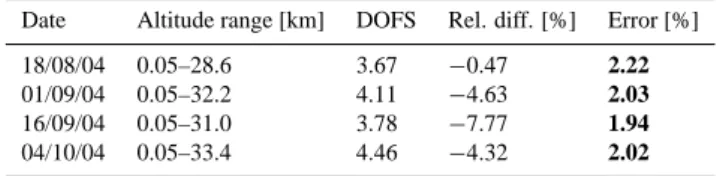
Table 5. Relative differences (in %) between O3partial columns from sonde and FTIR measurements at Ile de La R´eunion on coin-cident days. DOFS gives the number of degrees of freedom for the partial column in the high sensitivity altitude range of both instru-ments. The last column provides the random errors (in %) on the relative differences, calculated as 4 * [PCSonde* PCFTIR/ (PCSonde + PCFTIR)2] * sqrt (σSonde2 +σFTIR2 ).
Date Altitude range [km] DOFS Rel. diff. [%] Error [%] 18/08/04 0.05–28.6 3.67 −0.47 2.22
01/09/04 0.05–32.2 4.11 −4.63 2.03
16/09/04 0.05–31.0 3.78 −7.77 1.94
04/10/04 0.05–33.4 4.46 −4.32 2.02
a reference. To support the interpretation of the observed differences between the FTIR and correlative partial column data, we have evaluated the random errors associated with the relative differences, from a combination of the random errors on the FTIR and sonde or satellite partial columns. This combined error is calculated as 4 * [PCCOR * PCFTIR / (PCCOR + PCFTIR)2] * sqrt (σCOR2 +σFTIR2 ), where σCOR and σFTIRare the relative random errors on the correlative sonde or satellite and on the FTIR partial column, respec-tively. Note that the smoothing error contribution can be ne-glected in this evaluation, because we have first smoothed the higher vertical resolution profiles from the sonde or satellite measurements (Rodgers and Connor, 2003).
6.1.2 Ground-based FTIR versus ozone sonde
There are only four days during the second campaign on which O3soundings and FTIR measurements have both been carried out at Ile de La R´eunion. These are 18 August, 1 and 16 September, and 4 October 2004. The vertical profiles agree well in the high sensitivity altitude range. As an ex-ample, Fig. 13 shows the comparison of the O3profiles on 16 September 2004. The relative differences (in %) between the high sensitivity partial columns for all four days are sum-marized in Table 5, together with the number of DOFS for the partial column in the considered altitude range, and the percentage random errors on the relative differences (as de-fined in Sect. 6.1.1), from the combined sonde and FTIR ran-dom errors. Since the ranran-dom error budget for the ozone sondes was not given in the NDACC database, we used typ-ical values from the JOSIE-2000 report (Smit and Straeter, 2004): 5% in every layer from the ground up to 20 km, and 7% in the layers above. From Table 5, we deduce that the ground-based FTIR retrievals overestimate the amount of O3 between the surface and about 30 km by 0 to 8%. Of course, this conclusion is based on 4 coincidences only. For all days the combined error is slightly dominated by the sonde errors.
Fig. 13. Comparison of O3 vertical profiles at St.-Denis on 16 September 2004 obtained from ground-based FTIR (blue dia-monds) and O3sonde (yellow dots). Green triangles indicate the a priori FTIR profile and red stars the sonde profile smoothed by the FTIR averaging kernels.
6.1.3 Ground-based FTIR versus ACE-FTS
During the 2004 campaign, there have been five overpasses of ACE above Ile de La R´eunion: occultation sr5497 on 20 August, occultation ss6153 on 3 October, occultation ss6168 on 4 October, occultation ss6197 on 6 October, and occul-tation sr6485 on 26 October. For each of these occuloccul-tations we have compared the ACE-FTS profiles (version v2.2) with our ground-based FTIR data. Note that the profiles measured by the ACE-FTS occultation on October 26 do not reach al-titudes below 16.6 km. Therefore the resulting comparisons for that day are not very valuable, but we do include them for completeness.
We have calculated the relative differences between the FTIR and smoothed ACE-FTS partial column amounts of each measured target gas, defined as 2 * (PCACE– PCFTIR) / (PCACE+ PCFTIR)* 100, in the altitude range where both FTIR and ACE-FTS are sensitive.
Figure 14 shows examples of profile comparisons for CH4, HF, and HNO3on 20 August, for O3, N2O, CO and HCl on 4 October, and for C2H6on 6 October. The horizontal red lines indicate the altitude ranges of high sensitivity. Within these ranges the smoothed ACE-FTS profiles agree quite well with the FTIR profiles.
Table 6 lists all comparison results, for each species and each coincident occultation. The above defined relative par-tial column differences are given (in %), together with the combined random errors (in %) on these differences, calcu-lated as 4 * [PCACE* PCFTIR/ (PCACE+ PCFTIR)2] * sqrt (σACE2 +σFTIR2 ).
In the discussion of the comparisons with the ACE-FTS data we will not take into account the results on 26 October, because of their limited reliability.
26/10/04 16.6–47.4 3.19 2.83 0.90 CH4 20/08/04 7.0–28.6 1.35 −6.16 1.40 03/10/04 5.8–28.6 1.42 −5.08 1.37 04/10/04 8.2–28.6 1.20 −6.53 1.64 06/10/04 5.8–28.6 1.60 −0.22 1.34 26/10/04 16.6–28.6 0.56 2.03 11.16 N2O 20/08/04 5.8–25.0 1.75 −7.42 0.59 03/10/04 5.8–31.0 2.02 −3.14 0.72 04/10/04 8.2–31.0 1.70 −4.50 0.74 06/10/04 5.8–28.6 6.57 15.03 0.73 26/10/04 16.6–25.0 0.70 12.36 1.45 CO 20/08/04 7.0–19.0 1.19 −18.80 3.33 03/10/04 5.8–19.0 1.31 25.02 3.49 04/10/04 8.2–19.0 0.96 −17.82 3.27 26/10/04 16.6–20.2 0.10 −2.44 3.57 C2H6 20/08/04 8.2–20.2 0.88 −14.15 8.94 03/10/04 7.0–20.2 1.24 25.27 6.16 04/10/04 8.2–20.2 1.16 −37.19 7.08 06/10/04 7.0–19.0 0.78 −39.02 12.98 26/10/04 17.8–20.2 0.09 −47.75 19.22 HCl 20/08/04 8.2–47.4 1.38 10.16 4.10 03/10/04 9.4–42.4 1.28 30.31 3.37 04/10/04 9.4–42.4 1.28 15.08 3.41 06/10/04 8.2–47.4 1.25 −8.24 4.32 26/10/04 16.6–44.8 1.07 −22.73 2.58 HF 20/08/04 14.2–40.2 1.14 −3.41 3.12 26/10/04 17.8–38.2 1.07 −47.65 2.48 HNO3 20/08/04 16.6–32.2 0.93 3.41 4.67 03/10/04 16.6–28.6 1.09 25.93 4.73 04/10/04 16.6–28.6 1.09 5.59 4.80 06/10/04 16.6–32.2 1.03 −30.89 4.59 26/10/04 16.6–28.6 0.97 −49.62 4.05
For O3, the relative differences between ACE-FTS and ground-based FTIR vary between −14 and +12%, in the mid-dle troposphere (∼6 km) up to the stratopause (∼47 km). For CH4 and N2O, the relative differences between ACE-FTS and ground-based FTIR range from −7 to 0% and from −8 to +15%, respectively, in the middle troposphere up to about 30 km. For CO and C2H6, the upper altitude limit for the comparison is restricted to 20 km; the differences between ACE-FTS and ground-based FTIR vary between −19 and +25% for CO, and between −39 and +26% for C2H6. The altitude range for the comparison of HCl goes from the mid-dle troposphere to about the stratopause; the observed differ-ences range from −9 to +31%.
For HF, we have only one reliable comparison, namely on 20 August, for which the relative difference between the ACE-FTS and the ground-based FTIR partial column in the range 14 to 40 km is about −4%. Comparisons for HNO3 in the range 17 to 30 km, show differences between −31 and +26%.
In all mentioned comparisons, the variations in the ob-served differences are larger than what we expect on the basis of the random errors on the relative differences. For all species we see that the FTIR errors are equivalent to or slightly bigger than the ACE-FTS errors.
Table 7. Relative differences (in %) between HALOE and FTIR high sensitivity partial columns at Ile de La R´eunion in 2004 for each common measured species, together with the combined random error, defined as 4 * [PCHALOE* PCFTIR/ (PCHALOE+ PCFTIR)2] * sqrt (σHALOE2 +σFTIR2 )(in %).
Molecule Date Altitude range [km] DOFS Rel. diff. [%] Error [%]
O3 29/08/04 10.6–47.4 3.66 −12.34 1.64 30/08/04 10.6–47.4 3.54 −9.03 0.89 31/08/04 10.6–50.8 3.61 −14.82 0.92 14/09/04 10.6–42.4 3.32 −56.51 16.30 15/09/04 10.6–50.8 3.63 −13.09 0.90 16/09/04 10.6–47.4 3.46 −16.31 0.87 CH4 29/08/04 14.2–28.6 0.71 −6.86 10.71 30/08/04 14.2–28.6 0.70 −8.47 5.26 31/08/04 14.2–28.6 0.70 −5.22 5.37 14/09/04 14.2–28.6 0.69 −4.76 5.34 15/09/04 14.2–28.6 0.69 −5.57 7.97 16/09/04 14.2–28.6 0.72 −4.67 5.44 HCl 29/08/04 15.4–44.8 1.09 2.13 13.94 30/08/04 15.4–44.8 1.00 −7.86 8.87 31/08/04 15.4–23.8 1.91 −15.24 11.13 14/09/04 15.4–44.8 1.20 −47.09 1.94 15/09/04 16.6–47.4 0.74 −15.51 2.87 16/09/04 15.4–44.8 1.51 2.04 2.14 HF 29/08/04 15.4–40.2 1.15 −0.10 8.57 30/08/04 15.4–40.2 1.18 −8.30 2.97 31/08/04 15.4–40.2 1.17 −13.59 3.91 14/09/04 15.4–40.2 1.13 −45.44 4.80 15/09/04 15.4–38.2 1.11 −19.25 2.73 16/09/04 15.4–38.2 1.10 −1.06 4.36
6.1.4 Ground-based FTIR versus HALOE
In the same way as we did for ACE-FTS, we have com-pared our ground-based FTIR data with correlative data from HALOE. Conform to the ACE comparisons in this pa-per, we have calculated the relative differences between the FTIR and smoothed HALOE partial column amounts as 2 * (PCHALOE– PCFTIR)/ (PCHALOE+ PCFTIR)* 100, in the al-titude range where both FTIR and HALOE are sensitive for the target species.
Figure 15 shows examples of comparisons between re-trieved FTIR and the original and smoothed HALOE profiles of O3, CH4, HCl, and HF on 16 September 2004. The hori-zontal red lines indicate the altitude ranges of high sensitiv-ity. Analogue to the ACE-FTS comparisons, the smoothed HALOE profiles agree fairly well with the FTIR profiles within these ranges. Table 7 gives an overview of all compar-isons, for each species and each coincident occultation. The relative differences on the relevant partial column are given (in %), together with the associated DOFS and random er-ror (in %), defined as 4 * [PCHALOE* PCFTIR/ (PCHALOE+ PCFTIR)2] * sqrt (σHALOE2 + σFTIR2 ). It appears in Table 7 that the discrepancies between HALOE and ground-based FTIR partial columns are always larger on 14 September 2004 than on the other days. We have verified the HALOE and
ground-based FTIR data for that particular day and up to now, we haven’t found any good explanation for the large inconsis-tencies. We therefore don’t take into account that day in the current discussion.
For HCl and HF, in general, the HALOE partial columns in the range 15 to 45 km and 15 to 40 km, respectively, are smaller than the corresponding FTIR partial columns, by about 7 to 16% and 1 to 20%, respectively. This agrees to some extent with previous findings by Russell et al. (1996a, 1996b) saying that HALOE slightly underestimates the HCl and HF vmr profiles. In particular, they found that the mean difference between HALOE and correlative balloon mea-surements is better than 7% for HF and ranges from 8 to 19% for HCl, throughout most of the stratosphere. Following Russell et al. there appears to be a systematic offset between HALOE and ATMOS measurements ranging from 10 to 20% both for HF and HCl, and even reaching 40% for HF in the lower stratosphere. The differences between the HALOE and ground-based FTIR O3 partial columns in the range 10 to 47 km vary between 9 and 17%, with the HALOE profiles being smaller than the ground-based FTIR profiles. For CH4, the HALOE partial columns in the lower stratosphere (15 to 28 km) are smaller than the ground-based FTIR columns by about 4 to 9%.
(a) (b)
(c) (d)
(e) (f)
(g) (h)
Fig. 14. Vertical vmr profiles from 0 to 60 km of (a) O3on 4 October, (b) CH4on 20 August, (c) N2O on 4 October, (d) CO on 4 October, (e) C2H6on 6 October, (f) HCl on 4 October, (g) HF on 20 August, and (h) HNO3on 20 August, measured at St.-Denis in 2004 by ground-based FTIR (blue diamonds) and by ACE-FTS (raw: yellow circles; smoothed: red stars). The FTIR a priori profile is indicated by the green triangles.
(a) (b)
(c) (d)
Fig. 15. Vertical vmr profiles form 0 to 60 km of (a) O3, (b) CH4, (c) HCl and (d) HF, measured at St.-Denis by ground-based FTIR (blue diamonds) and by HALOE (raw: yellow circles; smoothed: red stars) on 16 September 2004. The green triangles indicate the a priori FTIR profile.
For O3and CH4the combined error is dominated by the FTIR errors, whereas for HCl and HF it is dominated by the HALOE errors.
6.2 Differential observations between Ma¨ıdo and St.-Denis The campaign in 2002 has allowed us to look at the species’ abundances in the about 2.15 km thick atmospheric bottom layer between St.-Denis and Ma¨ıdo. Unfortunately, only very few measurements could be made on exactly the same day at both sites, because of meteorological conditions.
Figure 16 shows the total column amounts (TC) of O3, CH4, N2O, CO, C2H6, HCl, HF, and HNO3, retrieved at Ma¨ıdo and at St.-Denis in 2002, together with their respective absolute differences, TCStDenis– TCMaido, and the combined random error on those differences, defined as sqrt (σStDenis2 * TC2StDenis+σMaido2 * TC2Maido), where σStDenisand σMaidoare the relative random error on the total columns at St.-Denis and Ma¨ıdo, respectively.
As expected, the total column amounts measured on the same day at both sites coincide within the error bars for the stratospheric species HCl, HF and HNO3. For the tro-pospheric species CH4, N2O, CO, and C2H6 there is a sig-nificant offset in their total columns, corresponding to their abundances in the atmospheric layer in between both
obser-vatories. For O3, there is also a small offset, confirming its non-zero concentration in the boundary layer.
Based on these differences between the column values at Ma¨ıdo and at St.-Denis, we can derive an estimate of the sur-face volume mixing ratios of the target species, assuming a constant vmr between 0.05 and 2.2 km. This is a good as-sumption for the well-mixed long-lived gases CH4and N2O, and a reasonable approximation for the other ones. Our thus obtained estimates are 1324 ppbv for CH4, 86 ppbv for CO, 265 ppbv for N2O, and 139 pptv for C2H6.
For CH4 and CO the values agree well (i.e., within the error bars) with the ones from the NOAA ESRL Globalview database (http://www.esrl.noaa.gov/gmd/ccgg/globalview/ co/co intro.html), namely about 1750 and 80 ppbv, respec-tively, at 20◦S in October, if we take into account the total uncertainties on the total column values, including the systematic uncertainties. Analogously, our estimate of the N2O surface concentration agrees reasonably well with the value of 316 ppbv at the Southern Hemisphere station of Cape Matatula (14◦S, 171◦W) in 2002, reported by Jiang et al. (2007).
(a) (b)
(c) (d)
(e) (f)
(g) (h)
Fig. 16. Upper plots: total column amounts (in molecules/cm2)together with random error bars of (a) O3, (b) CH4, (c) N2O, (d) CO, (e) C2H6, (f) HCl, (g) HF, and (h) HNO3, measured at Ma¨ıdo (blue crosses) and at St.-Denis (red circles) in 2002 by ground-based FTIR. Lower plots: absolute differences (in molecules/cm2)of the total column amounts, calculated as the St.-Denis column value minus the Ma¨ıdo one, together with their random error bars.