PLANNING AND MANAGEMENT OF CLOUD COMPUTING NETWORKS
FEDERICO LARUMBE
D´EPARTEMENT DE G´ENIE ´ELECTRIQUE ´
ECOLE POLYTECHNIQUE DE MONTR´EAL
TH`ESE PR´ESENT´EE EN VUE DE L’OBTENTION DU DIPL ˆOME DE PHILOSOPHIÆ DOCTOR
(G´ENIE ´ELECTRIQUE) SEPTEMBRE 2013
c
´
ECOLE POLYTECHNIQUE DE MONTR´EAL
Cette th`ese intitul´ee:
PLANNING AND MANAGEMENT OF CLOUD COMPUTING NETWORKS
pr´esent´ee par: LARUMBE Federico
en vue de l’obtention du diplˆome de: Philosophiæ Doctor a ´et´e dˆument accept´ee par le jury d’examen constitu´e de:
M. GIRARD Andr´e, Ph.D., pr´esident
Mme SANS `O Brunilde, Ph.D., membre et directrice de recherche M. EL HALLAOUI Issmail, Ph.D., membre
ACKNOWLEDGMENTS
This thesis has been possible thanks to the strong support of my research advisor Brunilde Sans`o that shared her knowledge, motivation, and resources as well as the creation of a lab with excellent people. I appreciate very much the availability and valuable comments of the jury Andr´e Girard, Issmail El Hallaoui, and Jean-Charles Gr´egoire. I am also very thankful for the help of my colleagues and friends Marnie Vodounou, Lˆe Nguyen, and Hadhami Dbira. This thesis has also been possible thanks to the Group for Research in Decision Analysis (GERAD) and Polytechnique Montr´eal that provided an environment with very bright people in optimization and telecommunication.
ABSTRACT
The evolution of the Internet has a great impact on a big part of the population. People use it to communicate, query information, receive news, work, and as entertainment. Its extraordinary usefulness as a communication media made the number of applications and technological resources explode. However, that network expansion comes at the cost of an important power consumption. If the power consumption of telecommunication networks and data centers is considered as the power consumption of a country, it would rank at the 5th place in the world. Furthermore, the number of servers in the world is expected to grow by a factor of 10 between 2013 and 2020. This context motivates us to study techniques and methods to allocate cloud computing resources in an optimal way with respect to cost, quality of service (QoS), power consumption, and environmental impact. The results we obtained from our test cases show that besides minimizing capital expenditures (CAPEX) and operational expenditures (OPEX), the response time can be reduced up to 6 times, power consumption by 30%, and CO2 emissions by a factor of 60.
Cloud computing provides dynamic access to IT resources as a service. In this paradigm, programs are executed in servers connected to the Internet that users access from their computers and mobile devices. The first advantage of this architecture is to reduce the time of application deployment and interoperability, because a new user only needs a web browser and does not need to install software on local computers with specific operating systems. Second, applications and information are available from everywhere and with any device with an Internet access. Also, servers and IT resources can be dynamically allocated depending on the number of users and workload, a feature called elasticity.
This thesis studies the resource management of cloud computing networks and is divided in three main stages. We start by analyzing the planning of cloud computing networks to get a comprehensive vision. The first question to be solved is what are the optimal data center locations. We found that the location of each data center has a big impact on cost, QoS, power consumption, and greenhouse gas emissions. An optimization problem with a multi-criteria objective function is proposed to decide jointly the optimal location of data centers and software components, link capacities, and information routing.
Once the network planning has been analyzed, the problem of dynamic resource provi-sioning in real time is addressed. In this context, virtualization is a key technique in cloud computing because each server can be shared by multiple Virtual Machines (VMs) and the total power consumption can be reduced. In the same line of location problems, we propose a Green Cloud Broker that optimizes VM placement across multiple data centers. In fact,
when multiple data centers are considered, response time can be reduced by placing VMs close to users, cost can be minimized, power consumption can be optimized by using energy-efficient data centers, and CO2 emissions can be decreased by choosing data centers provided
with renewable energy sources.
The third stage of the analysis is the short-term management of a cloud data center. In particular, a method is proposed to assign VMs to servers by considering communication traffic among VMs. Cloud data centers receive new applications over time and these applica-tions need on-demand resource provisioning. Each application is composed of multiple types of VMs that interact among themselves. A program called scheduler must place each new VM in a server and that impacts the QoS and power consumption. Our method places VMs that communicate among themselves in servers that are close to each other in the network topology, thus reducing communication delay and increasing the throughput available among VMs. Furthermore, the power consumption of each type of server is considered and the most efficient ones are chosen to place the VMs. The number of VMs of each application can be dynamically changed to match the workload and servers not needed in a particular period can be suspended to save energy.
The methodology developed is based on Mixed Integer Programming (MIP) models to formalize the problems and use state of the art optimization solvers. Then, heuristics are developed to solve cases with more than 1,000 potential data center locations for the plan-ning problem, 1,000 nodes for the cloud broker, and 128,000 servers for the VM placement problem. Solutions with very short optimality gaps, between 0% and 1.95%, are obtained, and execution time in the order of minutes for the planning problem and less than a second for real time cases. We consider that this thesis on resource provisioning of cloud computing networks includes important contributions on this research area, and innovative commercial applications based on the proposed methods have promising future.
R´ESUM´E
L’´evolution de l’internet a un effet important sur une grande partie de la population mon-diale. On l’utilise pour communiquer, consulter de l’information, travailler et se divertir. Son utilit´e exceptionnelle a conduit `a une explosion de la quantit´e d’applications et de ressources informatiques. Cependant, la croissance du r´eseau entraˆıne une importante consommation ´
energ´etique. Si la consommation ´energ´etique des r´eseaux de t´el´ecommunications et des cen-tres de donn´ees ´etait celle d’un pays, il se classerait 5e pays du monde. Pis, le nombre de serveurs dans le monde devrait ˆetre multipli´e par 10 entre 2013 et 2020. Ce contexte nous a motiv´e `a ´etudier des techniques et des m´ethodes pour affecter les ressources d’une fa¸con optimale par rapport aux coˆuts, `a la qualit´e de service, `a la consommation ´energ´etique et `a l’impact ´ecologique. Les r´esultats que nous avons obtenus minimisent les d´epenses d’investissement (CAPEX) et les d´epenses d’exploitation (OPEX), r´eduisent d’un facteur 6 le temps de r´eponse, diminuent la consommation ´energ´etique de 30% et divisent les ´emissions de CO2 par un facteur 60.
L’infonuagique permet l’acc`es dynamique aux ressources informatiques comme un service. Les programmes sont ex´ecut´es sur des serveurs connect´es `a l’internet, et les usagers peuvent les utiliser depuis leurs ordinateurs et dispositifs mobiles. Le premier avantage de cette ar-chitecture est de r´eduire le temps de mise en place des applications et l’interop´erabilit´e. En effet, un nouvel utilisateur n’a besoin que d’un navigateur web. Il n’est forc´e ni d’installer de programmes sur son ordinateur, ni de poss´eder un syst`eme d’exploitation sp´ecifique. Le deuxi`eme avantage est la disponibilit´es des applications et de l’information de fa¸con continue. Celles-ci peuvent ˆetre utilis´ees `a partir de n’importe quel endroit et de n’importe quel dis-positif connect´e `a l’internet. De plus, les serveurs et les ressources informatiques peuvent ˆetre affect´es aux applications de fa¸con dynamique, selon la quantit´e d’utilisateurs et la charge de travail. C’est ce que l’on appelle l’´elasticit´e des applications.
Cette th`ese ´etudie l’allocation des ressources des r´eseaux infonuagiques et elle est divis´ee en trois ´etapes principales. Nous analysons en premier lieu la planification des r´eseaux infonuagiques pour avoir une vision compl`ete. La premi`ere question `a r´esoudre concerne la localisation optimale des centres de donn´ees. Nous montrons que leur position a un impact important sur les coˆuts, sur la qualit´e de service, sur la consommation ´energ´etique et sur les ´emissions de gaz `a effet de serre. Nous proposons un probl`eme d’optimisation avec une fonction `a plusieurs objectifs pour d´ecider simultan´ement des positions des centres de donn´ees, de celles des applications, des capacit´es des liens et du routage de l’information.
r´eel. Dans ce contexte, la virtualization est une technique tr`es importante parce qu’elle permet d’utiliser un seul serveur comme support physique de plusieurs machines virtuelles (MVs). La consommation ´energ´etique totale est alors r´eduite. Dans cette optique, on propose aussi un syst`eme qui optimise le positionnement des MVs sur plusieurs centres de donn´ees. Ainsi, lorsque l’on consid`ere plusieurs centres de donn´ees, on constate que le temps de r´eponse est r´eduit quand les MVs sont plac´ees pr`es des utilisateurs, que le coˆut est r´eduit pour des fournisseurs meilleur march´e, la consommation ´energ´etique est moindre pour les centres de donn´ees ayant une bonne utilisation de l’´energie, et les ´emissions de CO2peuvent ˆetre r´eduites
en choisissant des centre de donn´ees utilisant une ´energie verte.
La troisi`eme ´etape de l’analyse porte sur la gestion des ressources d’un centre de donn´ees. Une m´ethode est propos´ee pour affecter des MVs aux serveurs en tenant compte de la commu-nication entre les MVs et les variations de la charge de travail. Un centre de donn´ees re¸coit des applications les unes apr`es les autres, et doit satisfaire leurs demandes en ressources. Chaque application est compos´ee de plusieurs types de MVs qui interagissent entre elles. Un programme appel´e ordonnanceur doit placer chaque nouvelle MV sur un serveur. Ceci a un impact sur la qualit´e de service et la consommation ´energ´etique. La m´ethode propos´ee place les MVs devant communiquer entre eux pr`es les unes des autres. Ainsi, le d´elai de communication est r´eduit et le d´ebit disponible entre les MVs est augment´e. De plus, la consommation ´energ´etique de chaque type de serveur est prise en compte et les serveurs les plus efficaces sont choisis pour h´eberger les VMs. La quantit´e de MVs de chaque application est modifi´ee de fa¸con dynamique selon la charge de travail et les serveurs qui ne sont pas n´ecessaires `a un moment donn´e sont mis en veille pour ´epargner de l’´energie.
La m´ethodologie d´evelopp´ee se base sur des mod`eles de programmation en nombre entiers pour formaliser les probl`emes et pour utiliser les solveurs `a l’´etat de l’art. Des heuristiques sont d´evelopp´ees pour r´esoudre des cas avec plus de 1,000 centres de donn´ees possibles pour le probl`eme de planification, plus de 1,000 noeuds pour le probl`eme d’affectation de MVs aux centres de donn´ees et 128,000 serveurs pour l’affectation de MVs aux serveurs. Les solutions trouv´ees ont des intervalles d’optimalit´e tr`es petits, entre 0 et 1.95%. Le temps d’ex´ecution est de l’ordre de quelques minutes pour le probl`eme de planification et moins d’une seconde pour les cas en temps r´eel. Nous consid´erons que cette th`ese sur l’allocation de ressources des r´eseaux infonuagiques apporte des contributions importantes `a ce domaine de recherche, et des applications commerciales bas´ees sur les m´ethodes propos´ees ont un avenir prometteur.
TABLE OF CONTENTS DEDICATION . . . iii ACKNOWLEDGMENTS . . . iv ABSTRACT . . . v R´ESUM´E . . . vii TABLE OF CONTENTS . . . ix
LIST OF TABLES . . . xiii
LIST OF FIGURES . . . xiv
LIST OF ACRONYMS AND ABREVIATIONS . . . xvi
CHAPITRE 1 INTRODUCTION . . . 1
1.1 Research objectives . . . 2
1.2 Problems studied . . . 3
1.3 Contributions . . . 13
1.4 Document structure . . . 13
CHAPITRE 2 LITERATURE REVIEW: LOCATION AND PROVISIONING PROB-LEMS IN CLOUD COMPUTING NETWORKS . . . 14
2.1 Definitions and base concepts . . . 14
2.1.1 Applications and computing background . . . 14
2.1.2 Cost and power consumption . . . 16
2.1.3 Performance parameters . . . 18
2.2 Data Center Location Problem (DCLP) . . . 21
2.2.1 Current approaches . . . 22
2.2.2 Analysis . . . 26
2.3 Dynamic scaling . . . 27
2.3.1 Current approaches . . . 29
2.3.2 Analysis . . . 31
2.4.1 Current approaches . . . 34
2.4.2 Analysis . . . 39
2.5 Virtual machine placement within a data center . . . 40
2.5.1 Current approaches . . . 41
2.5.2 Analysis . . . 47
2.6 Conclusion . . . 48
CHAPITRE 3 ARTICLE 1: A TABU SEARCH ALGORITHM FOR THE LOCATION OF DATA CENTERS AND SOFTWARE COMPONENTS IN GREEN CLOUD COMPUTING NETWORKS . . . 50 3.1 Introduction . . . 51 3.2 Related work . . . 53 3.3 Problem description . . . 55 3.3.1 Network traffic . . . 56 3.3.2 Servers . . . 58 3.3.3 Energy . . . 59 3.3.4 Cost . . . 60 3.3.5 Decision variables . . . 61 3.3.6 Objective function . . . 61 3.3.7 Constraints . . . 63 3.4 Solution approach . . . 65 3.4.1 Solution space . . . 65 3.4.2 Initial solution . . . 67 3.4.3 Neighborhood relation . . . 68 3.4.4 Tabu list . . . 69 3.4.5 Stop criterion . . . 70 3.5 Case study . . . 70
3.5.1 Network and application topology . . . 70
3.5.2 Network traffic . . . 70
3.5.3 Servers . . . 71
3.5.4 Power . . . 71
3.5.5 Cost . . . 71
3.6 Results . . . 72
3.6.1 Trade-off between objectives . . . 72
3.6.2 Comparison between tabu search and Cplex . . . 75
3.7 Conclusion . . . 79
CHAPITRE 4 ARTICLE 2: GREEN CLOUD BROKER, DYNAMIC VIRTUAL MA-CHINE PLACEMENT ACROSS MULTIPLE CLOUD PROVIDERS . . . 81
4.1 Introduction . . . 82
4.2 Related work . . . 85
4.3 Problem description . . . 87
4.3.1 Network topology, application, and meta-scheduler . . . 87
4.3.2 Communication traffic . . . 91
4.3.3 VMs and dynamic scaling . . . 91
4.3.4 Cost . . . 92
4.3.5 Energy and environment . . . 92
4.3.6 System variables . . . 93 4.3.7 Objective function . . . 93 4.3.8 Constraints . . . 94 4.4 Solution approach . . . 96 4.5 Case study . . . 98 4.5.1 Network topology . . . 98 4.5.2 Application topology . . . 99 4.5.3 Communication traffic . . . 100 4.5.4 Dynamic workload . . . 100 4.5.5 Servers . . . 100
4.5.6 Power consumption and greenhouse gas emissions . . . 100
4.5.7 Cost . . . 101
4.6 Results . . . 101
4.6.1 Experience procedure . . . 101
4.6.2 The set of experience . . . 101
4.6.3 Setting . . . 101
4.6.4 Relation between delay, power, CO2, and cost over time . . . 101
4.6.5 Application workload during the day . . . 105
4.6.6 Execution time . . . 108
4.7 Conclusion . . . 110
CHAPITRE 5 ONLINE, ELASTIC, AND COMMUNICATION-AWARE VIRTUAL MACHINE PLACEMENT WITHIN A DATA CENTER . . . 111
5.1 Virtual machine placement strategy . . . 111
5.1.2 Communication . . . 114
5.1.3 Energy efficiency . . . 115
5.1.4 Elasticity . . . 115
5.2 Problem description . . . 116
5.2.1 Network topology . . . 116
5.2.2 Applications and scheduler . . . 116
5.2.3 Communication traffic . . . 118 5.2.4 Servers . . . 118 5.2.5 VMs . . . 119 5.2.6 Power consumption . . . 119 5.2.7 Elasticity . . . 120 5.2.8 System variables . . . 120 5.2.9 Objective function . . . 121 5.2.10 Constraints . . . 122 5.3 Solution approach . . . 125 5.4 Case study . . . 127
5.4.1 Network topology, delay, and throughput . . . 127
5.4.2 Application topology . . . 127 5.4.3 Servers . . . 128 5.4.4 Power consumption . . . 128 5.5 Results . . . 129 5.5.1 Initial period . . . 129 5.5.2 Workload . . . 130 5.5.3 Execution time . . . 132 5.6 Discussion . . . 134 5.7 Conclusion . . . 135
CHAPITRE 6 GENERAL DISCUSSION . . . 136
6.1 Applications . . . 137
6.2 Scalability . . . 138
6.3 Service architecture . . . 139
6.4 Elasticity . . . 139
CHAPITRE 7 CONCLUSION AND RECOMMENDATIONS . . . 140
LIST OF TABLES
Table 1.1 Three stage approach of cloud network planning and management. . . 12
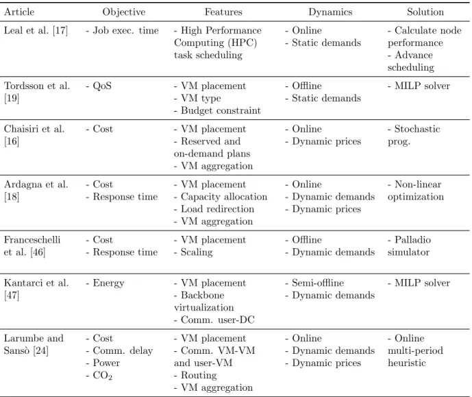
Table 2.1 Data center location approaches. . . 23
Table 2.2 Dynamic scaling approaches. . . 28
Table 2.3 Meta-scheduling approaches. . . 35
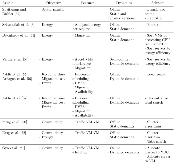
Table 2.4 Virtual machine placement approaches. . . 42
Table 3.1 Data center location and provisioning approaches. . . 54
Table 3.2 Solutions for 10 cities with up to 10 data centers. . . 74
Table 3.3 Comparison between tabu search and Cplex. Delay priority. . . 76
Table 3.4 Comparison between tabu search and Cplex. CO2 priority. . . 76
Table 3.5 Comparison between tabu search and Cplex. Cost priority. . . 76
Table 3.6 Tabu search results for large cases. Delay priority. . . 77
Table 3.7 Tabu search results for large cases. Pollution priority. . . 77
Table 3.8 Tabu search results for large cases. Cost priority. . . 77
Table 5.1 Cloptimus Scheduler vs First-Fit after adding 800 applications. . . 130
LIST OF FIGURES
Figure 1.1 Energy consumption of countries and the cloud. Adapted from Cook [1]. 3
Figure 1.2 Data center location and software component placement. . . 4
Figure 1.3 Cloud Network Planning Problem (CNPP) parameters, constraints, and solution. . . 5
Figure 1.4 Meta-scheduler parameters, constraints, and solution. . . 8
Figure 1.5 Actors and components interacting in the life-cycle of cloud applications. 8 Figure 1.6 VM placement parameters, constraints, and solution. . . 11
Figure 2.1 Server virtualization layout. . . 15
Figure 2.2 System power approximation. Adapted from Fan et al. [2]. . . 17
Figure 2.3 Data Center Location Problem (DCLP). . . 21
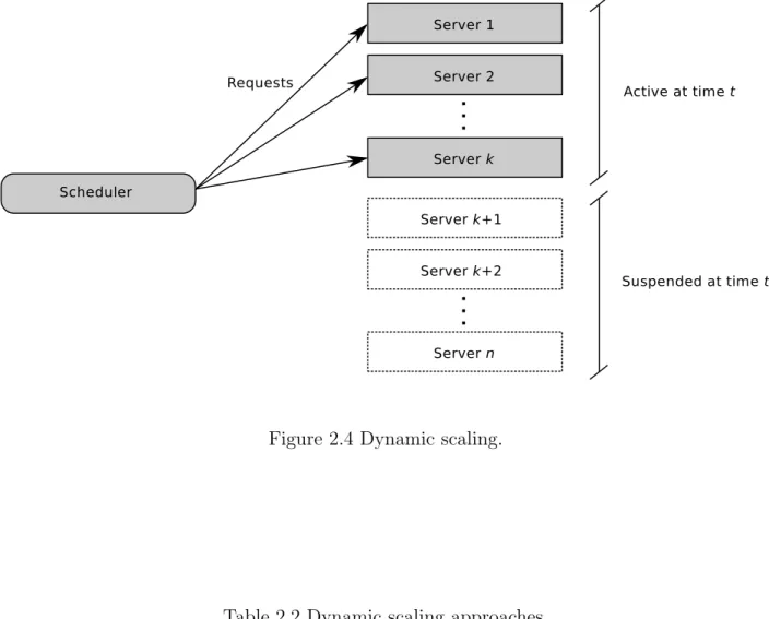
Figure 2.4 Dynamic scaling. . . 28
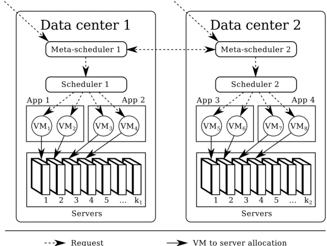
Figure 2.5 Meta-scheduling architecture. . . 32
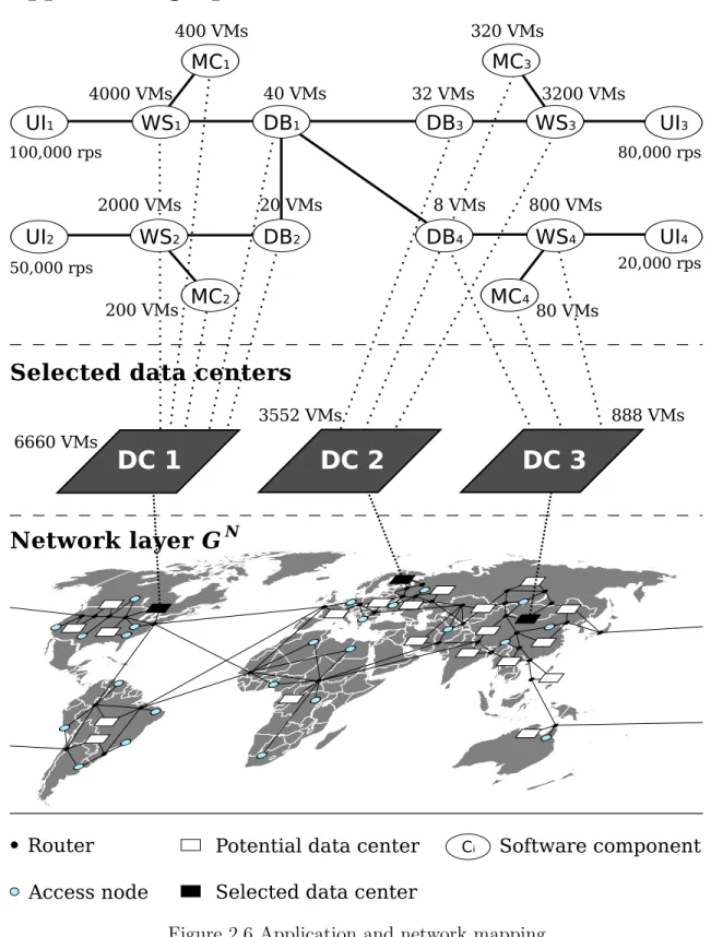
Figure 2.6 Application and network mapping. . . 38
Figure 2.7 Energy consumption per service request. Adapted from Srikantaiah et al. [3]. . . 44
Figure 3.1 Network and application layers. . . 57
Figure 3.2 Greedy solution for the web search engine example. . . 69
Figure 3.3 Network topology with 10 cities and 10 potential data centers. . . 72
Figure 3.4 Solution A. Delay minimization. . . 73
Figure 3.5 Solution B. Pollution minimization. . . 73
Figure 3.6 Solution C. Cost minimization. . . 73
Figure 3.7 Tabu search vs greedy heuristic for large cases and cost priority. . . . 79
Figure 4.1 Energy consumption of countries and the cloud. Adapted from Cook [1]. 83 Figure 4.2 Actors and components interacting in the life-cycle of cloud applications. 83 Figure 4.3 Application and network mapping. . . 88
Figure 4.4 Network topology with the largest 100 cities in terms of Internet users. Image generated with Google Maps API. . . 99
Figure 4.5 Delay over time. . . 103
Figure 4.6 Trade-off between delay and cost. . . 103
Figure 4.7 Power consumption over time. . . 104
Figure 4.8 Trade-off between power consumption and cost. . . 104
Figure 4.9 CO2 emissions over time. . . 106
Figure 4.11 Data center power consumption. . . 107
Figure 4.12 Spike in the number of VMs when prices are changed. . . 107
Figure 4.13 Low data center utilization when prices are changed. . . 108
Figure 4.14 Average meta-scheduler execution time over the network size. . . 109
Figure 4.15 Average meta-scheduler execution time over the application size. . . . 109
Figure 5.1 Graph of a multi-tier application. . . 112
Figure 5.2 Data center network topology. . . 113
Figure 5.3 Application and network mapping. . . 117
Figure 5.4 San Jose CAIDA’s traffic monitor during August 3, 2013 [4]. . . 128
Figure 5.5 Server power consumption. . . 129
Figure 5.6 Number of VMs used and power consumption in each period. . . 131
Figure 5.7 Average scheduler execution time over the application size. . . 133
LIST OF ACRONYMS AND ABREVIATIONS
API Application Programming Interface
AS Autonomous System
CAPEX Capital expenditures CDN Content Delivery Network
CNPP Cloud Network Planning Problem CPU Central Processing Unit
CS Cloptimus Scheduler
DB Database
DCLP Data Center Location Problem
DVFS Dynamic Voltage and Frequency Scaling
FF First Fit
FIFO First in First Out
GCBP Green Cloud Broker Problem HPC High Performance Computing
ICT Information and Communications Technology ISP Internet Service Provider
IXP Internet Exchange Point IaaS Infrastructure as a Service
LAN Local Area Network
LHC Large Hadron Collider
MCDA Multi Criteria Decision Analysis
MILP Mixed Integer Linear Programming MIP Mixed Integer Programming
MSE Mean Square Error
NASA National Aeronautics and Space Administration OPEX Operational expenditures
OXC Optical cross-connect PUE Power Usage Effectiveness PaaS Platform as a Service rps Requests per second
QAP Quadratic Assignment Problem QoE Quality of experience
QoS Quality of service
SLA Service Level Agreement SaaS Software as a Service
ToR Top of Rack
UI User Interface
VDC Virtual Data Center
VM Virtual Machine
CHAPTER 1
INTRODUCTION
In 1963, researchers discussed the possibility of connecting some research institutes’ comput-ers to share resources, programs, and information. Licklider [5] called it the Intergalactic Computer Network, and in the same memo that describes the network, the author asked if a program to plot functions should be downloaded from a remote computer and executed locally, or if the data should be sent to the remote computer that stores the program, execute it there, and then download the results. This shows that location of data and programs has been an architectural issue for a long time. Some years later, in 1969, the two first nodes of the ARPANET, precursor of the Internet, were connected. Though the technology was at its beginnings, its creators already envisioned that computing could be accessed as an utility from homes and offices in the same way as electricity and telephone [6]. Over the years, the Internet has expanded and computers have increased their capacity exponentially. At the end of the 1980s, scheduling algorithms were developed to execute tasks on multiple processors, a concept known as High Performance Computing (HPC). By the late 1990s, grid computing became popular when general middlewares executed HPC applications on multiple independent clusters [7]. At the same time, the world wide web rapidly arose and massive web sites became available. Internet data centers grew and multiple commercial models appeared to provide computing resources.
The concept of providing computing as an utility is currently known as cloud comput-ing [8]. Cloud services can be classified in three service models dependcomput-ing on what are the ac-tions of clients and providers. In Infrastructure as a Service (IaaS), a client pays for accessing raw IT resources managed by a provider: processing power, network bandwidth, storage. The client is responsible for maintaining the software, and the infrastructure provider manages the hardware and the computing facility. In Platform as a Service (PaaS), a provider installs commonly used software such as operating systems, programming environments, databases, and load balancers. Then, each client develops applications in a programming environment such as Python, Java, and .NET in the given platform. The third cloud computing model is called Software as a Service (SaaS), and it is what we use everyday. The client uses appli-cations given by the provider such as e-mail, social networks, spreadsheets, word processors, and photo editors.
Providers store data and execute applications in computers hosted in facilities called data centers. Users access applications from their computers and mobile devices. The Internet
provides access between client devices and servers composed of cellular antennas, wireless routers, modems, routers, optical links, and optical cross connects.
1.1 Research objectives
In the present thesis, we propose planning and management methods to improve the following aspects of cloud computing networks:
Quality of Service (QoS)
As people use more cloud applications, high availability and short response time become increasingly important. The response time is composed of the server execution time and the time to send information between servers and client devices. The first one depends on the server capacity and the complexity of the program executed. The communication delay is associated to the transmission delay, queuing delay, and propagation delay. The transmission delay is inversely proportional to the network interface capacity. The queuing delay is the time that information packets wait while other packets are being served in each router between the client and the server. The propagation delay is the time that electrical and optical signals take to travel each link.
Cost
In the planning and management of cloud computing networks, cost is a fundamental met-ric [9]. Providers are interested in paying the least possible while achieving the expected QoS. The cost is composed of capital expenditures (CAPEX) and operational expendi-tures (OPEX). CAPEX are costs that create future benefits, including servers, routers, optical links, and data centers. OPEX are the ongoing costs for running the system: electric-ity, the water used for cooling, IT staff, security guards, administrative staff, and external providers. Costs can be minimized with a planning that reduces the amount of resources needed, and an efficient resource management to reduce power consumption.
Power consumption
Each network element consumes power over time. If the power consumption of global telecom-munication networks and data centers was considered as the power consumption of a country, it would rank as the 5th country of the world, as can be seen in Figure 1.1. More precisely,
a large data center can consume the same energy as 80,000 American households or 250,000 European ones [1]. Given that projections predict a multiplication of the number of servers
0 1000 2000 3000 4000 US China Russia Japan Cloud India Germany Canada France
Electricity consumption (billion kWh)
Figure 1.1 Energy consumption of countries and the cloud. Adapted from Cook [1].
by a factor of 10 between 2013 and 2020 [10], resources must be optimally allocated to applications in order to limit the growth of power consumption.
Greenhouse gas emissions
Besides controlling power consumption, reducing CO2 emissions is also needed given their
impact on global warming. In fact, the method of power generation has a big impact on the amount of CO2 emitted: 10 g of CO2 per kWh are produced by wind and hydroelectric
power, 38 g / kWh by geothermic energy, 66 g / kWh by nuclear power, 778 g / kWh by diesel, and 960 g / KWh by coal [11]. Therefore, the type of energy used greatly impacts the greenhouse gas emissions, and these emissions increase the global warming.
1.2 Problems studied
This thesis optimizes the objectives described above in multiple stages: 1) planning the network of data centers, 2) coordinated management of multiple data centers, 3) internal management of each data center. As we will see, the proposed models have a common structure but the decisions in each of them are taken at different times and have different duration.
Cloud Network Planning Problem (CNPP)
The method first developed for this thesis optimizes the planning of an infrastructure provider network. More precisely, we study how data center location impacts on cost, quality of
service (QoS), power consumption, and CO2 emissions. In fact, cost is reduced when data
centers with low energy and land prices are chosen, the QoS is improved when data centers are placed close to users, power consumption is reduced with data centers in cold climate, and CO2 emissions are dramatically reduced in regions where green energy is available. A Mixed
Integer Linear Programming (MILP) model is presented with an objective function that combines multiple criteria with priority coefficients. Planners can change these coefficients to analyze multiple solutions making trade-offs that depend on their priorities.
We state the problem as a mapping between two graphs: an application layer GA and a network topology GN. Each node in GAis a software component, and each arc (i, j) represents the fact that software component i sends information to software component j. The network layer is composed of access nodes, backbone routers, potential data center locations, and the links that connect these nodes. The optimization model must decide for each software component in GA, which node in GN it is assigned to. Then, the nodes in GN that will
host software components must be open, e.g., if a solution places software components in a data center, then this data center is selected. Each software component may require to be executed in multiple servers (e.g., a thousand) and there is a capacity constraint in each data center. Also, each communication demand in GA represents a flow of information packets
that must be routed through GN.
Figure 1.2 shows an example of a global application provider with users in four different regions: 1) North America, 2) Latin America, 3) Europe and Africa, and 4) Asia and the Pacific. The network layer is composed of potential data centers, backbone routers, and access nodes that aggregate users. The application is composed of a user interface that is executed on the client computers, a web service, and a database. The application is further split by region, as shown at the top of the figure. There is one web service responding to the users in each region, a database replica for each region, and a user interface for each access node. The arcs of the application graph are communication demands between the software components: traffic between the user interfaces and web services, between the web services and databases, and between the databases and master database. The problem consists of selecting a subset of the potential data centers and deciding which data center will host each web service and database. Furthermore, each web service is executed on multiple servers. Thus, placing a software component in a data center means that we must also allocate servers for that purpose without exceeding the data center capacity. The solution for this example was to select two of the potential data centers: one in Europe and one in Asia. The users from North America, Latin America, and Europe are served from the data center located in Europe, and the users in Asia obtain cloud services from the data center located in that region.
The comprehensive planning problem summarized in Figure 1.3 simultaneously answers the following questions:
• Among a set of potential data center locations, which ones should be used to open new data centers?
• Which data center should host each of the software components of the cloud applica-tions?
• How many servers will be hosted at each data center? • How will the information be routed through the network? • What are the link capacities required to carry that information?
The MILP model was first solved with AMPL/Cplex for cases with up to 12 access nodes and 24 potential data center locations. An exhaustive research was done to define all the parameters based on realistic values and public data [9]. The relation between cost, response time, power consumption, and CO2 emissions was studied for that kind of networks. However,
the case of 24 data center locations took 58 minutes to solve, and we were interested in solving cases with 1,000 data center locations because the largest global networks have that kind of size [12]. Thus, we developed a tabu search heuristic [13] to handle large cases. Comparing the solutions of the small cases to the optimal solutions gave as a result optimality gaps between 0 and 1.95%, and most of them were below 0.1%. The case of 24 potential data centers was solved by the heuristic in 868 milliseconds, while Cplex took 58 minutes. The case of 1,000 potential data centers was solved in 10 minutes and was unsolvable in Cplex.
As we will see in Chapter 2, few authors specifically addressed the problem of data center location. Our work first differentiates in the flexible representation of each application as a graph of software components. That representation precisely defines the communication pattern of any kind of applications, that is very valuable to plan distributed applications. Our model also uses a detailed calculation of cost, communication delay, power consumption, and CO2 emissions, and it is also flexible to allow planners to define priorities. Furthermore,
even if it is difficult to compare our technique with other work, because they solve different models, our heuristic took 21 seconds to solve an instance with 500 data centers and the work most closely related [14] solved a case with the same number of data centers in 30 minutes in a similar environment.
Figure 1.4 Meta-scheduler parameters, constraints, and solution.
Meta-scheduling: resource allocation across multiple data centers
Once the network is defined, the every day management of the cloud computing system has also an impact on cost, QoS, power consumption, and CO2 emissions. In the same line of
location problems, we analyzed the online placement of software components across multiple data centers, a process called meta-scheduling. In this case, the system has a set of data centers already open, and applications arrive consecutively. Furthermore, the application workload presents daily fluctuations with periods of high and low utilization. The dynamic provisioning of resources, or dynamic scaling, allocates resources needed by each application at each time instead of reserving a large amount of resources for peak periods.
That dynamism can be well managed through virtualization technique [15], where each physical server executes one or multiple Virtual Machines (VMs). In this case, instead of using each server for a single purpose, it can host different VMs over time: A web service VM during the day to serve users’ HTTP requests and a HPC application overnight to process big amounts of data and generate statistics. In fact, each software component is executed on a different number of VMs in each period of the day, and all the VMs use the same shared pool of servers in a data center.
The problem that is solved at this stage takes place at the time of deploying a new application. A meta-scheduler must choose a data center to host the VMs of each software component taking into account dynamic workload variations. That impacts the cost because different data centers have different VM prices. It also impacts the power consumption because the servers used for the VMs will consume energy, and each data center has a Power Usage Effectiveness (PUE) that accounts for the overhead of cooling and power distribution. The CO2 emissions change depending on the type of energy that provides the data center.
As summarized in Figure 1.4, this optimization problem minimizes costs by answering the following question:
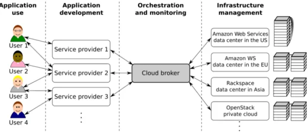
• Which data center will host each software component’s VMs in each period of the day, given the expected workload, expected performance, and current network state? The problem was stated from the point of view of a cloud broker, that is, an intermediate entity between the service providers that need to execute applications and the infrastructure providers that offer computing capacity, as can be seen in Figure 1.5. A cloud broker is a program that manages resources of multiple data centers belonging to one or more providers in a unique platform. Commercial cloud brokers exist—e.g., RightScale, Enstratius, Grav-itant, and Scalr—, but they lack a meta-scheduler to help users optimally place software components. There is some work that addresses the meta-scheduler problem [16, 17, 18, 19].
Our proposal adds several contributions with respect to these approaches, including spe-cial considerations for communication traffic between users and VMs which is important for distributed cloud applications, multi-period dynamic scaling, and CO2 emission reductions.
The solution approach is an online and multi-period heuristic based on a tabu search algorithm. The cases solved had more than 1,000 nodes, 650 applications, and 6,500 VMs. Results show that the application response time can be reduced up to 6 times as compared with using the cheapest data center, 30% of power consumption can be saved, and CO2
emissions can be reduced by 60 times. The execution time to determine the optimal software component placement of an application took between a few milliseconds to less than a second, making the program suitable to be embedded in an interactive cloud broker platform. VM placement within a data center
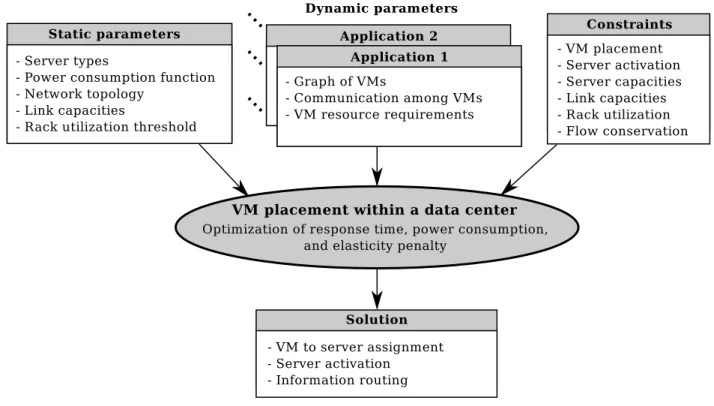
A third stage in the process of resource provisioning of cloud computing networks is the management of each particular data center. In this context, the problem to solve is which server should host each VM. Figure 1.6 summarizes the features of the proposed Mixed Integer Programming (MIP) model. The objective is to minimize response time and power consumption subject to capacities of server resources. Similarly to the previous two stages, we emphasize that the VMs of an application can communicate among themselves. VMs that communicate among themselves can be placed in nearby servers to reduce delay and increase the bandwidth globally available among VMs.
In this problem, the dynamic aspect is very important. Cloud providers receive new appli-cations over time, and a program called scheduler must allocate resources to each application. That is, when a new application arrives, each VM must be placed in one of the servers. Each server can host multiple VMs, and the servers that are not hosting VMs can be put in sleep mode to save power. Furthermore, the workload of an application can change over the day, with periods of high and low activity, so that the number of VMs in an application can be changed to match the dynamic workload.
Many authors have studied the problem of VM placement within a data center, but only a few of them took special attention to the communication among VMs [20, 21, 22]. Our contribution is a method that considers both communication among VMs and a dynamic workload. We take advantage of the hierarchic topology of data centers to propose a hierarchic tabu search heuristic that can scale to more than 100,000 servers and VMs.
The test cases analyzed show encouraging results: the transmission delay is reduced by 70% and link utilization decreases up to 33% compared to methods that do not consider traffic; the power consumption is reduced by 4.9% representing $1.6 millions savings per year in a data center with 128,000 servers. This means that our approach increases the quality
Figure 1.6 VM placement parameters, constraints, and solution.
of service by placing VMs that communicate among themselves in nearby servers, reducing delay and the utilization of links among switches.
Common structure
The three problems in planning and resource management have a common mathematical structure that is customized for each stage. Table 1.1 summarizes the main features of each problem that result in a mapping between an application graph GAand a network GN. That
is, for each node in GA, a node in GN is chosen, and for each arc in GA, network paths are used to carry the information. This is shown in the first two constraints of each problem in Table 1.1.
In the first stage, each node in GA is a software component, and the nodes in GN are
potential data centers, access nodes, and routers. The potential data centers in GN that host
software components in a particular solution are the locations where new data centers will be opened. The communication delay is minimized and optimal links capacities are assigned, important aspects when planning a network. That is the reason why we include routing and link capacity assignment decisions. Given that when a location is chosen, a data center
Table 1.1 Three stage approach of cloud network planning and management.
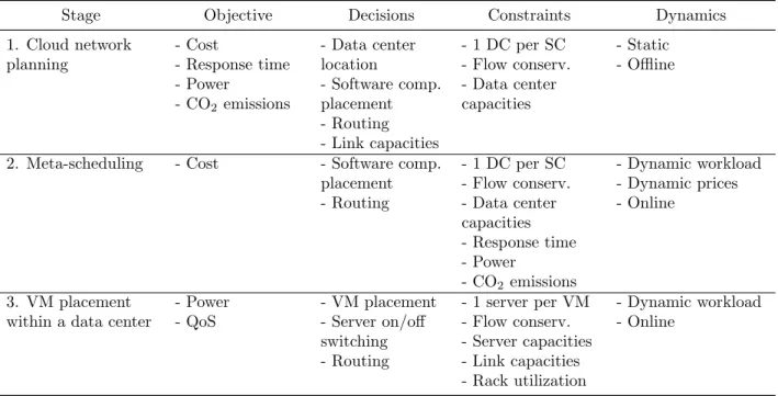
Stage Objective Decisions Constraints Dynamics
1. Cloud network planning - Cost - Response time - Power - CO2emissions - Data center location - Software comp. placement - Routing - Link capacities - 1 DC per SC - Flow conserv. - Data center capacities - Static - Offline
2. Meta-scheduling - Cost - Software comp. placement - Routing - 1 DC per SC - Flow conserv. - Data center capacities - Response time - Power - CO2 emissions - Dynamic workload - Dynamic prices - Online 3. VM placement within a data center
- Power - QoS - VM placement - Server on/off switching - Routing - 1 server per VM - Flow conserv. - Server capacities - Link capacities - Rack utilization - Dynamic workload - Online
remains open in that location for several years, the planning problem is offline with static expected demands.
The second stage is to place applications across multiple data centers, that is, to choose the optimal data center for each software component. The graphs GA and GN are similar to the
first stage with the difference that each software component requires a number of VMs, and we know which data centers are open. The decision of software component placement can change more often because deploying a software component is much less expensive that opening a data center. Furthermore, the workload of each software component changes over the day. That is the reason why we propose an online and dynamic optimization engine. To schedule a new application, residual data center capacities must be considered and the optimization is solved for multiple periods. In this case, the response time, power consumption, and CO2
emissions were expressed as constraints to analyze how cost increases when the constraints are tighter.
Finally in stage three, the elements to place are the VMs that compose each application within a particular data center. In this case, each VM is placed in a server to minimize power consumption and improves the QoS. The workload changes over the day and the deployment of a new application must be done taking into account existing applications that are already being executed.
1.3 Contributions
The following is the list of contributions of this thesis:
1. A mixed integer programming framework for the location of cloud elements through a mapping between an application and a network graph.
2. Definition of the CNPP for planning cloud networks taking into account the cost, QoS, power consumption, and CO2 emissions.
3. A tabu search heuristic for the CNPP that achieves near optimal solutions in short execution time.
4. Definition of the Green Cloud Broker Problem (GCBP) to produce the meta-scheduling of distributed applications across multiple data centers.
5. An online and multi-period heuristic for the GCBP that optimizes application deploy-ments in less than a second.
6. Definition of a VM placement problem that handles traffic among VMs and elasticity of applications.
7. A hierarchic tabu search heuristic to schedule new applications and resize existing ones, handling cases of more than 100,000 servers and VMs in real time.
1.4 Document structure
The remainder of this document is structured as follows. Chapter 2 presents a literature review on cloud network planning and management. The articles closest to ours are analyzed as well as related problems of dynamic provisioning. Chapter 3 presents the paper Larumbe and Sans`o [23] that defines the CNPP and the proposed tabu search heuristic. Chapter 4 presents the Green Cloud Broker for the dynamic placement of VMs across multiple providers as in Larumbe and Sans`o [24]. Chapter 5 studies the dynamic placement of VMs in servers to optimize QoS and power consumption. Chapter 6 explains how the approaches can be integrated to achieve the objectives of energy consumption, pollution, quality of service, and cost minimization. Chapter 7 concludes the research on cloud network planning and dynamic provisioning and proposes future avenues of research and development.
CHAPTER 2
LITERATURE REVIEW: LOCATION AND PROVISIONING PROBLEMS IN CLOUD COMPUTING NETWORKS
This chapter presents a literature review on planning and management of cloud comput-ing networks 1. In this chapter, we discuss the problems mentioned in the introduction, analyze various methods to find optimal solutions, and present our contributions in each area. In Section 2.1, some definitions necessary to the understanding of the problems are presented. In that section, the general problem setting and relevant metrics are defined. Then, Section 2.2 discusses the Data Center Location Problem (DCLP) in the context of planning cloud computing networks. Section 2.3 describes dynamic scaling architectures and algorithms to determine the number of Virtual Machines (VMs) needed for each application in each period of the day. That section presents the concept of scheduling within a data center which is a prerequisite of scheduling. Section 2.4 reviews articles about meta-scheduling to manage resources of multiple data centers in a coordinated fashion. Section 2.5 presents papers about the placement of VMs in servers within a data center. Finally, the chapter concludes with the current state of the location and provisioning problems in cloud computing.
2.1 Definitions and base concepts
This section is devoted to an overview on the common background of the problems that will be treated in this thesis. Such a background can be divided in three groups related to: 1) the applications and the computing environment, 2) the way energy is consumed and cost are evaluated and, finally, 3) users and performance issues.
2.1.1 Applications and computing background Applications
Object-oriented programming is currently a very widespread programming paradigm. In this paradigm, a program is conceived as a set of objects that interact by sending messages. The objects can be hosted on a single computer or distributed across a computer network. When
1This chapter appears in Communication infrastructures for cloud computing: design and applications
edited by Hussein Mouftah and Burak Kantarci. Copyright 2013, IGI Global, www.igi-global.com. Posted by permission of the publisher.
Figure 2.1 Server virtualization layout.
the objects are on the same computer, the messages are exchanged through the CPU and the RAM. Objects on different computers can communicate using protocols that convert the message into information packets, which are sent through links and routers connecting the two ends. In the client/server architecture, the program is split into a component that is executed on a client device and a component that is executed on a server. In practice, the client component is replicated, and multiple users can connect to the same server. Similarly, the server component can be replicated when a single server is not sufficient to efficiently process the user requests. The users can connect from their homes or offices using their phones, tablets or computers. The servers are hosted in large data centers to take advantage of economies of scale. Complex applications contain not only a client and a server but also a set of software components, each with its own specific purpose. For example, a popular social network can present the following set of software components: 1) a Javascript client that is executed in the user desktop browsers, 2) a client for smart phones, 3) a web server for answering HTTP requests, 4) a database that stores the user posts on hard disks, 5) a system to send and receive messages, and 6) file servers for picture storage. All these software components send messages to each other to accomplish the global purpose of the application.
Virtual machines
Between the software and hardware levels, there is an element known as the Virtual Machine (VM). A VM is a program that simulates the behavior of a computer. Similar to a computer, it has access to processing units, RAM memory, hard disks, and devices. However, these elements are provided by a system known as the hypervisor, which is executed on the physical machine hosting the VM. As shown in Figure 2.1, any operating system can be installed on a VM, and the operating system is unaware that it is being executed on a virtual rather than a physical machine. The user programs interact with the operating system as usual. The hypervisor ensures that the VMs are isolated from each other and have the necessary resources. Using a virtualization framework offers many advantages to the cloud computing paradigm. An infrastructure provider can offer VMs to its customers and consolidate multiple VMs on a single server. Because many applications require fewer resources than an entire server, the server consolidation reduces the number of servers, cost, and energy consumption. 2.1.2 Cost and power consumption
CAPEX and OPEX
Each element of the cloud network has a purchasing cost, setup cost, and amortization period [9]. The server cost varies depending on the components: the CPU, capacity of the hard disks, RAM, and motherboard. In addition to servers, the routers, optical fiber, and optical repeaters contribute to cost, and the cost of the power distribution equipment, cooling equipment, data center building, and land must also be considered. To compute the total cost of all the elements, ranging from an individual server to the entire data center, the cost of each element is divided by its amortization period and then added to the sum. For instance, the amortization period of a server is between 3 and 4 years and that of a data center is between 12 and 15 years [9]. All the costs listed so far comprise the capital expenditures (CAPEX). In addition to the CAPEX, there are the operational expenditures (OPEX), including electricity, the water used for cooling, the IT staff to maintain the equipment, security guards, and administrative staff.
Power consumption
Each active network element consumes power. The power consumed by a server is the sum of the power consumed by its components. The Central Processing Unit (CPU) typically consumes the majority of the power, and depends on the degree of utilization. When the CPU is idle, the consumption is reduced. Figure 2.2 shows an example of the system power consumption as a function of its utilization [2]. The function is monotonically increasing, has
0 p min p max 0% 20% 40% 60% 80% 100% System power (W) CPU utilization
Figure 2.2 System power approximation. Adapted from Fan et al. [2].
a value of pmin when the utilization is zero and reaches pmax when the utilization is 100%.
Depending on the server architecture, operating system, and hypervisor used, the consump-tion when the server is idle may be as high as 70% of the maximum power consumpconsump-tion. The consolidation of VMs in servers is therefore a promising strategy because suspending servers that are not highly utilized saves a large amount of power. The definite integral of the server power consumption over a given time interval is the total energy used during that period. The equipment used to distribute the power in the data centers has fixed limits on the total power consumption. For example, a row of 450 servers in a data center may have a maximum capacity of 150 KW. The active ports of the routers consume power, as do the optical cross-connects (OXCs) and optical repeaters. The power distribution and cooling equipment also consumes power, and the consumption rate determines the efficiency of the data center. The Power Usage Effectiveness (PUE) is defined as the ratio of the total power consumed by a data center to the power consumed by the IT equipment. For instance, a PUE of 1.15 means that the base equipment for cooling and power distribution requires 15% of the IT equipment requirement. The most efficient data centers may reach a PUE of 1.07 using mechanisms that exploit the surrounding climate for cooling. OpenCompute is a consortium of companies that promote the open design of efficient IT equipment and data centers by publishing the technologies used to achieve high data center efficiency [25].
generation mechanism: whether it is renewable and how much environmental pollution is introduced in the production process. Wind and hydroelectric power produce approximately 10 g of CO2 per KWh. Geothermic energy production introduces 38 g of CO2 per KWh,
diesel produces 778 g / KWh, and coal produces 960 g / KWh [11]. The type of energy used by a data center therefore greatly impacts the pollution level.
2.1.3 Performance parameters Response time and throughput
As we have seen, the software components communicate by exchanging messages among themselves. When a software component receives a message, we call it a request. The software component processes the request, potentially sending messages to other components, and answers with a message called a response. The time elapsed between the reception of the request and the response is called the response time. The inverse of that value is the throughput, which is the number of requests per second that a software component can process.
Communication delay
The messages exchanged between the software components are typically sent through a net-work protocol such as TCP and UDP over IP, which generates information packets that traverse the network. These packets pass through paths of routers and links between the source and destination hosts. Each router is connected to its links through network inter-faces. When a router receives a packet, its header is analyzed, and then the packet is placed in the interface corresponding to the output link. The time of that operation is called the processing delay. If the output interface also had other packets to send, then the packet is placed in an output queue. The period between the reception of the packet in the output queue and the time when the packet is sent is called the queuing delay, and the time required to place each bit of the packet in the transmission channel is called the transmission delay. The time from the placement of the packet in the transmission channel to the moment when it is completely received on the other end is the propagation delay. That delay depends on the physical properties of the transmitting medium, e.g., the speed of light in optical fiber is approximately 200,000 km/s. The sum of all of these delays yields the delay of a seg-ment router-link, and the sum of the delays of the segseg-ments in a network path is called the communication delay.
Availability
Hardware failures, software maintenance, and upgrades can prevent a service from responding to requests during specified periods. The availability is the proportion of time that a service is functional. For instance, we can say that the availability of an e-mail service was 99.99% in the last week. The same concept is applied to hardware elements such as servers, routers, and links. It can also be applied to an entire data center, e.g., the average availability of a data center may be 99.99% [9]. When applications are executed on multiple servers at the same time, the service availability increases because the failure of a single server has a lower impact. The availability can also be improved by avoiding single failure points in the network and using backup paths when a link or router fails.
Service Level Agreement (SLA)
The metrics discussed above impact the quality of service (QoS) that an operator provides to its customers. Customers and providers use SLAs to keep the metrics above (or below) a specified threshold. When the metric is outside their range, the provider must compensate the customer. A mechanism to monitor the metrics must also be defined, and tools must be developed to query and visualize the metrics in real time and over the history of the system. The models in this chapter typically aim to minimize the utilization of resources and satisfy the SLAs.
Workload forecasting
The models to plan and manage cloud computing networks require the workload size of each application as an input in order to determine the type and number of servers and VMs needed. The first issue that planners need to solve is to know the characteristics of the workload. Typically, there is a small number of applications that generate most of the traffic. Identifying these applications and their software components is needed. Then, for each application component, the workload can be split into different types of transactions depending on the objects exchanged, e.g., text, images, and videos.
Furthermore, the workload can change over time. The number of application requests per second over time can be displayed in a chart to analyze the workload. Some patterns that could arise are: increasing workload, decreasing, stationary, and/or with seasonal, weekly or daily fluctuations. For instance, a workload could increase over the year because new users are registered, and at the same time could vary over the day with peaks in specific hours.
There are two complementary classes of methods to forecast the workload of applications: qualitative and quantitative [26]. Delphi [27, 28] is a qualitative method where the
expecta-tions of actors in the organization and users are taken into account. In this case, business level metrics such as the number of orders per month are used to allow all the actors to participate in the forecast process. Then, the agreed forecast in terms of business metrics is translated to system level metrics, e.g., requests per second. Quantitative metrics use the workload history to predict the future workload. For instance, the workload of each hour of the day can be predicted taking into account the workload of previous days at the same hour. The workload of each week day can be calculated using the same week day of previous weeks.
Three quantitative techniques to estimate workloads can be highlighted [26]: 1. Regression methods,
2. Moving average, and 3. Exponential smoothing
Regression methods estimate a variable value as a function of other variables. Given a set of actual data points that measure the independent and dependent variables, the function that best approximates these values is searched. Linear regression searches for the linear function that minimizes the sum of square errors of each sample. This method can be used to translate business metrics into system metrics. For instance, the number of orders can be counted in each hour as well as the maximum number of requests per second in each hour. From that data set, linear regression can be used to obtain the relation between the number of orders and requests per second.
Moving average calculates a metric to forecast as the average of that same metric in n previous periods. For instance, the maximal number of requests per second for the next 10 minutes could be calculated as the average of the same metric in the three previous periods of 10 minutes. The method must be calibrated by defining the right duration and number of periods.
Exponential smoothing also takes the variable value in the previous periods to predict a new value, with the difference that a coefficient multiplies each value to decrease older values, and give more priority to last values. To compare approximations of different techniques and parameters, the Mean Square Error (MSE) can be used.
To summarize, capacity planning requires to know the workload in detail, the main appli-cations, the type of transactions, and to use qualitative and quantitative metrics to forecast the future workload on multiple timescales.
Figure 2.3 Data Center Location Problem (DCLP).
2.2 Data Center Location Problem (DCLP)
Data center location is the main decision to make in the Cloud Network Planning Problem (CNPP) that we proposed. In this section, we classify existing papers that address the DCLP including the articles that are part of this thesis.
QoS is a top priority because of the increasing use of cloud computing applications for personal and business tasks: to search for information, news, communication between people, social networks, entertainment. The delay between the user computers and the servers that host programs and information has a big impact on QoS. That delay is associated to the path composed of routers and links between a user computer and a data center. Thus, different data center locations produce different delays: when the data centers are closer to the users, the propagation delay is smaller and there are fewer intermediate routers adding queuing and transmission delay. Thus, cloud providers open data centers in multiple regions to locate the applications as close as possible to the users. For instance, the largest content delivery network Akamai has more than 1,000 small data centers around the world hosting images, videos, and applications for a large number of organizations [12].
minimize the delay experienced by user applications. Figure 2.3 shows an example. Users are aggregated as access nodes that demand services from the cloud. In this example, there are six access nodes. Very often, the choice of data center location is not totally open, but there are potential locations that are considered by the planner. In the figure example, there are six potential data center locations. Three of these locations were selected to place a data center and the service demands were routed from the access nodes to the data centers.
Delay is not the only issue impacted by the location of the data center. In fact, data center location has also an impact on costs such as the price of the land, electricity price, and the cost of environmental pollution that is produced by the type of energy—wind, solar, hydroelectric, nuclear, diesel, coal—that is available. For an effective data center location planning model, trade-offs between locations with low land costs, energy prices, CO2
emis-sions and the proximity to the users should be used. In fact, from the cost minimization perspective, the optimal is to open a few data centers in cheap locations; from the delay minimization perspective, the best is to open many data centers near the users. On the other hand, to minimize CO2 emissions the best solution is to open data centers only in locations
where green energy is available.
This problem has an exponential number of possible solutions as a function of the potential locations, making necessary to use integer programming models, optimization solvers, and optimization techniques. In the following subsections we first present a review on a set of variants for this base problem. Finally, in the last subsection, we provide an analysis for further research on the topic.
2.2.1 Current approaches
Table 2.1 summarizes the most significant work relating to the DCLP. In the second column, the articles are classified by the type of objective to be minimized: communication delay, cost, energy consumption, pollution, social environment, and risks. The third column refers to the decision that can be reached when using the proposed model: data center location, assignment of access nodes to data centers, routing of traffic demands, and application lo-cation. In the final column, the different solutions approaches are portrayed: Mixed Integer Linear Programming (MILP) models solved with commercial solvers, simulated annealing heuristic [33], tabu search heuristic [13], Linear Programming (LP), and the classification method ELECTRE TRI [34].
Table 2.1 Data center location approaches.
Article Objective Decisions Solution
Chang et al. [29] - Delay - DC location - AN to DC assig. - AN to backup DC
MILP solver
Goiri et al. [14] - Cost - DC location - AN to DC assig.
Simulated annealing + LP
Dong et al. [30] - Energy - DC location - AN to DC assig. - Routing
MILP solver
Larumbe and Sans`o [31] - Delay - Cost - Pollution - DC location - AN to DC assig. - App. location - Routing MILP solver
Larumbe and Sans`o [23] - Delay - Cost - Pollution - DC location - AN to DC assig. - App. location - Routing - Link capacities Tabu search
Covas et al. [32] - Risk - Social - Cost - Pollution
- DC location ELECTRE TRI
Delay minimization with backup coverage
The first variant to the DCLP is to minimize the average delay between access nodes and data centers subject to a budget constraint and the assignment of backup data centers. A data center can fail for many reasons: energy outage, link cuts, router failures, remote attacks, software errors. Redundancy such as multiple network links and energy lines diminish the probability of failure and increases the availability. The probability of natural disasters must also be considered. One way to protect against this is to replicate cloud services in multiple data centers and have mechanisms to route the service demands to a backup data center when the primary fails. Chang et al. [29] proposed an integer programming model where each access node must be assigned to a primary data center and a backup data center. The study also considered the load of each data center, defined as the sum of the demand that it serves. The maximal load in a solution is the load of the data center with the largest demand. The maximal load was added to the objective function that is minimized. The lowest value that the maximal load can take is when all the loads are the same. That is why that strategy tends to balance the load between all the selected data centers.
Cost minimization
Another variant to this problem is to minimize the total network cost subject to QoS con-straints. In this case, the service demand of an access node can be assigned to a potential data center only if the delay between the access node and the data center is lower than a fixed parameter. Goiri et al. [14] proposed a model to solve this variant and studied potential locations in the US considering energy and land costs. In addition, the expected availability of each data center, i.e., its expected available time over total time, was also considered. The combination of data centers in the solution must satisfy a minimum availability requirement for the entire system. The authors proposed a simulated annealing heuristic [33] combined with a linear programming model, and demonstrated that the optimal placement of data centers can save capital expenditures (CAPEX) and operational expenditures (OPEX). Energy consumption minimization
Network elements such as IP routers and optical switches consume energy. Different data center locations imply different routing and thus a different amount of energy consumed by the network. Dong et al. [30] studied the minimization of the optical and IP router power consumption as a function of the data center location using linear programming models. They also analyzed the efficiency of locating data centers close to renewable energy sources versus transporting the renewable energy to the data centers. Since transporting energy over the grid provokes losses, there is an incentive to place data centers near energy sources. The cases analyzed presented reductions of 73% in consumed energy. Of course, this approach could increase the delay because data centers can be farther from the users than the delay optimization case, but locating data centers near green energy sources and cold climate is a strategy used by companies such as Facebook that recently built a data center based on hydroelectric energy in Sweden [35].
Delay, cost, and pollution minimization
There are different types of energy to power a data center—solar, wind, hydroelectric, nu-clear, diesel, coal—and depending on the type, the CO2 emissions will vary. For instance,
hydroelectric power produces 10 g of CO2 per KWh and coal produces 960 g of CO2 per
KWh [11]. Thus, a data center with 60,000 servers located in a place where hydroelectric power is available will produce much less pollution than one with the same number of servers but powered with coal. The DCLP oriented towards pollution reduction should minimize the CO2 emissions of the whole network.
All these objectives—delay, cost, pollution—should be taken into account by the planners to analyze the DCLP from multiple perspectives. One way to address this is to embed all objectives into a multi-criteria function having one term per aspect, normalized in monetary terms. Thus, the delay penalty represents the cost of delay increase, for instance, the loss in revenues because of a worsening QoS. Pollution costs may come from regulatory penalties or loss in company image for using dirty energy. Finally, there are the traditional OPEX and CAPEX costs. In order to have an overall view on the trade-offs, planners can adjust penalties to analyze solutions in a comprehensive way.
Larumbe and Sans`o [31] solved this problem through a MILP model that minimizes a multi-objective function composed of a communication delay penalty, the data center CAPEX, the data center OPEX, the server cost, the energy cost and a pollution penalty. Larumbe and Sans`o [23] developed a tabu search heuristic for that problem. In these articles, the data center location was simultaneously solved with the placement of distributed appli-cations, making the problem more general and flexible. The application layer is modeled as a graph of software components that exchange traffic. In this case, the decisions include which data centers to use in addition to which data center will host each software component. Risk, social, economic and environmental criteria
Another approach to decide a data center location is to classify every potential location in multiple independent dimensions. Instead of assigning a unique monetary value to each location, a category Excellent (C1), Very good (C2), Acceptable (C3), or Bad (C4) is assigned to each criterion. The criteria to analyze include:
- Risk: flooding, earthquakes, fire, nuclear, crime. - Social: life quality, life cost, skilled labor.
- Economic: investment costs, operational costs, attractiveness to customers. - Environmental: renewable energy, free cooling, reuse of waste heat.
For instance, a location with no flooding risks, earthquakes, and with low criminality may be classified as C1 in the Risk criteria. However, it can be classified as C4 in the economic criteria due to high investment and operational costs. Covas et al. [32] used Multi-Criteria Decision Analysis (MCDA) techniques [34] to evaluate possible locations of a data center for Portugal Telecom. This approach has the advantage of not combining multiple criteria in a single monetary value, allowing the analysts the evaluation of the solutions. The disadvantage is that the delay between the final users and the data centers was not taken into account.
![Figure 1.1 Energy consumption of countries and the cloud. Adapted from Cook [1].](https://thumb-eu.123doks.com/thumbv2/123doknet/2335782.32649/20.918.273.644.104.396/figure-energy-consumption-countries-cloud-adapted-cook.webp)
![Figure 2.7 Energy consumption per service request. Adapted from Srikantaiah et al. [3].](https://thumb-eu.123doks.com/thumbv2/123doknet/2335782.32649/61.918.179.746.379.789/figure-energy-consumption-service-request-adapted-srikantaiah-et.webp)
