Optimization Models for the Joint Power-Delay Minimization Problem in Green Wireless Access Networks

HAL Id: hal-01241530

https://hal.archives-ouvertes.fr/hal-01241530

Submitted on 1 Jan 2016

HAL is a multi-disciplinary open access

archive for the deposit and dissemination of

sci-entific research documents, whether they are

pub-lished or not. The documents may come from

teaching and research institutions in France or

abroad, or from public or private research centers.

L’archive ouverte pluridisciplinaire HAL, est

destinée au dépôt et à la diffusion de documents

scientifiques de niveau recherche, publiés ou non,

émanant des établissements d’enseignement et de

recherche français ou étrangers, des laboratoires

publics ou privés.

Optimization Models for the Joint Power-Delay

Minimization Problem in Green Wireless Access

Networks

Farah Moety, Samer Lahoud, Bernard Cousin, Kinda Khawam

To cite this version:

Farah Moety, Samer Lahoud, Bernard Cousin, Kinda Khawam. Optimization Models for the Joint

Power-Delay Minimization Problem in Green Wireless Access Networks. Computer Networks, Elsevier,

2015, 92, Part 1, pp.148 - 167. �10.1016/j.comnet.2015.09.032�. �hal-01241530�

Optimization Models for the Joint Power-Delay Minimization Problem in Green

Wireless Access Networks

Farah Moetya_{, Samer Lahoud}a_{, Bernard Cousin}a_{, Kinda Khawam}b

a_{IRISA labs, University of Rennes I, Rennes, France}

b_{PRISM Labs, University of Versailles Saint-Quentin-en-Yvelines, France}

Abstract

In wireless access networks, one of the most recent challenges is reducing the power consumption of the network, while preserving the quality of service perceived by users. Hence, mobile operators are rethinking their network design by considering two objectives, namely, saving power and guaranteeing a satisfactory quality of service. Since these objectives are conflicting, a tradeoff becomes inevitable. We formulate a multi-objective optimization with aims of minimizing the network power consumption and transmission delay. Power saving is achieved by adjusting the operation mode of the network base stations from high transmit power levels to low transmit levels or even sleep mode. Minimizing the transmission delay is achieved by selecting the best user association with the network base stations. In this article, we cover two different technologies: IEEE 802.11 and LTE. Our formulation captures the specificity of each technology in terms of the power model and radio resource allocation. After exploring typical multi-objective approaches, we resort to a weighted sum mixed integer linear program. This enables us to efficiently tune the impact of the power and delay objectives.

We provide extensive simulations for various preference settings that enable to assess the tradeoff between power and delay in IEEE 802.11 WLANs and LTE networks. We show that for a power minimization setting, a WLAN consumes up to 16% less power than legacy solutions. A thorough analysis of the optimization results reveals the impact of the network topology, particularly the inter-cell distance, on both objectives. For an LTE network, we assess the impact of urban, rural and realistic deployments on the achievable tradeoffs. The power savings mainly depend on user distribution and the power consumption of the sleep mode. Compared with legacy solutions, we obtained power savings of up to 22.3% in a realistic LTE networks. When adequately tuned, our optimization approach reduces the transmission delay by up to 6% in a WLAN and 8% in an LTE network.

Keywords: Wireless access networks, Optimization, Power Consumption, Transmission Delay, User Association.

1. Introduction

In recent years, green radio has been increasingly emphasized for not only ecological concerns but also for signif-icant economic incentives. Information and Communication Technology (ICT) accounts for around 3% of the world’s annual electrical energy consumption and 2% of total carbon emissions. Moreover, it is estimated that ICT energy consumption is rising at 15 to 20 %, doubling every five years [1]. In 2008 this corresponded to about 60 billion kWh of electrical energy consumption and about 40 million metric tons of CO2 [2]. As a branch of the ICT sector, mobile networks are responsible for 0.2% of these emissions [3]. In addition to the environmental impacts, mobile operators are interested in reducing energy consumption for economic reasons, especially with increasing energy costs becoming a significant portion of mobile operator expenditure. Moreover, the recent explosive growth of the number of mobile devices and the consequent mobile internet traffic all produce continually high energy consumption. This calls for green solutions to address the challenges in energy-efficient communications. Operators have focused on

Email addresses:farah.moety@irisa.fr(Farah Moety),samer.lahoud@irisa.fr(Samer Lahoud),

technological developments in the past years to meet capacity and Quality of Service (QoS) demands for User Equip-ment (UE). Pushed by the needs to reduce energy, mobile operators have recently been rethinking network design for optimizing energy efficiency and satisfying user QoS requirements.

Currently, over 80% of the power in mobile telecommunications is consumed by the radio access network, more specifically at the base station (BS) level [4]. Hence, many research activities focus on improving the energy efficiency of wireless access networks. In the following, we give an overview of these activities and classify them according to different approaches that run at different timescales.

Planning and deployment: The planning of efficient wireless networks and the deployment of

energy-aware BSs deal with the problem of determining the positioning of BSs, the type (e.g., macro, micro, pico or femto) and the number of BSs needed to be deployed. In this context, we find that heterogeneous networks have gained great attention in current research. Precisely, deploying small and low-power BSs co-localized with macro cells is believed to decrease power consumption compared to high-power macro BSs. Moreover, it extends the coverage area of the macro BS where signals fail to reach distant UEs. Furthermore, small cells increase the network capacity in areas with very dense data usage. Planning and deployment tasks are performed at very coarse temporal levels, ranging from a few months to possibly years.

Cell sizing: Also known as cell breathing, cell sizing is a well-known concept that enables balancing traffic load

in cellular telephony [5, 6]. When the cell becomes heavily loaded, the cell zooms in to reduce its coverage area, and the lightly loaded neighboring cells zoom out to accommodate the extra traffic. Many state-of-the-art techniques are used to implement cell sizing, such as adjusting the transmit power of a BS, cooperating between multiple BSs, and using relay stations and switching BSs for sleep/off mode. Cell sizing is performed at medium temporal levels, ranging from hours to days.

User Association: User association is the functionality devoted to deciding the BS (macro, micro, pico or femto)

with which a given user will be associated in a heterogeneous network [7, 8]. The challenge is to optimize for example the delay, throughput, or network cost. User association is impacted by the cell sizing tasks: when an active BS is switched off or changes its transmit power level in a homogeneous network, users may need to change their associations. Many metrics are considered for selecting the serving BS, such as the received signal quality (Signal-to-Noise Ratio (SNR) or the corresponding achievable rate), the traffic load, or the distance between BS and UE, etc. User association is performed at small temporal levels, ranging from seconds to minutes.

Scheduling: Scheduling algorithms allocate the radio resources in wireless access networks, where the objectives

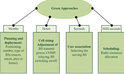
consist of improving the network throughput, satisfying the delay constraints of real-time traffic, or achieving fair resource distribution among users. Scheduling is performed at very short temporal levels of an order of few millisec-onds. In Figure 1, we illustrate the different green approaches studied in the state-of-the art as well as their operating timescales.

Reducing power consumption in wireless networks is coupled with satisfying the QoS requirements (delay, block-ing probability, etc.). As these objectives are conflictblock-ing, a tradeoff becomes ineluctable. Chen et al. [9] identified four key tradeoffs of energy efficiency with network performance: i) deployment-energy efficiency to balance the deploy-ment cost, throughput, and energy consumption in the network as a whole; ii) spectrum-energy efficiency to balance the achievable rate and energy consumption of the network; iii) bandwidth-power to balance the utilized bandwidth and the power needed for transmission; and iv) delay-power to balance the average end-to-end service delay and av-erage power consumed in transmission.

The delay-power tradeoff has not been studied deeply in the literature except for in a few recent cases [10]. In this article, we address the multi-objective optimization problem of power saving and transmission delay minimization in wireless access networks. Specifically, power saving is achieved by adjusting the operation mode of the network BSs from high transmit power levels to low transmit power levels, or even sleep mode. In this context, changing the op-eration mode of the BSs is coupled with optimized user association. Such coupling makes solving the problem more challenging. Minimizing the transmission delay is achieved by selecting the best user association with the network BSs.

State-of-the-art power saving approaches studied can also be performed in Wireless Local Area Networks (WLANs). Although power consumption of a cellular network BS is much higher than that of a WLAN Access Point (AP), the large number of APs deployed in classrooms, offices, airports, hotels and malls, contributes to a rapid increase in the power consumption in wireless access networks. Hence, efficient management of the power consumed by a WLAN is an interesting challenge. In the present article, we cover two different wireless networks: WLANs with IEEE 802.11g

Green Approaches Planning and deployment: Positioning, number, type of BSs (macro, micro, pico or femto). Cell sizing: Adjustment of BS transmit power, COMP, relaying, BS switching on/off. User association: Selecting the serving BS Scheduling: Radio resources allocation Hours Seconds Milli-seconds Months

Figure 1: Green approaches at different timescales.

technology and cellular networks with Long Term Evolution (LTE) technology.

Our approach presents multiple novelties compared to the state-of the art, and our main contributions are summa-rized as follows:

• We formulate the multi-objective optimization problem of power saving and delay minimization in wireless access networks, going beyond prior work which has focused on either minimizing energy without considering the delay minimization [4, 11, 12, 13, 14], or on delay analysis without accounting for energy minimization [7, 8]. Hence, the novelty in our approach is that it does not only strive to save energy by reducing the network power consumption, but also considers the minimization of the transmission delay.

• Unlike most of the literature studies, we combine different green approaches (BS on/sleep mode, adjustment of BS transmit power, user association) retaining advantages of each approach to provide power savings.

• We cover IEEE 802.11 and LTE technologies. To the best of our knowledge, our formulation is the first one that captures the specificity of each technology in terms of the power model and radio resource allocation (fair-rate sharing and fair-time sharing). In the WLAN scenario, considering the fair-rate scheduler, the delay model provided is a unique feature of our work, and it is a realistic model used in IEEE 802.11 WLAN [7, 8, 15] compared to the pessimistic bound of the queuing delay model used in the literature. In the LTE scenario, we consider a flat channel model with the fair-time scheduler.

• To solve the multi-objective optimization problem, we resort to the weighted sum method by combining the multiple objectives into a single objective scalar function. This method allows us to investigate the power-delay tradeoffs by tuning the weights associated with each objective.

• Starting from a binary non-linear formulation of the problem, we provide a MILP formulation of our problem that makes it computationally tractable. We obtain optimal results for both WLAN and LTE scenarios. The aim of the present paper is to study the different optimization models for the joint Power-Delay minimization problem in green wireless access networks. Such study brings a value to help in designing distributed solutions for the joint problem of power saving and delay minimization. Precisely, the optimal solution of the problem allows for an assessment and evaluation of any distributed solution. Moreover, the proposed formulation allows investigating the power-delay tradeoffs by tuning the weights associated with the power and delay objectives. This is an important feature of our model allowing it to reflect various preferences (i.e., saving power, minimizing delay or balance the tradeoff between minimizing power and delay). Thus, we can integrate the objective function of the joint Power-Delay

minimization problem in any practical algorithm (based on known heuristic algorithms such as simulated annealing, etc.) [16, 17].

The rest of the article is organized as follows. The performance metrics in green wireless networks are provided in Section 2. The different studied approaches to improve the energy efficiency of wireless access networks are presented in Section 3. The definitions and notations, used throughout the article, are introduced in Section 4. The Power-Delay multi-objective problem is formulated in Section 5. The network model is described in Section 6 with the models adopted for traffic, perceived rates, delay and power in IEEE 802.11 WLANs and LTE networks. The multi-objective optimization approach for WLANs and LTE cases are presented in Section 7. The methods for solving the multi-objective optimization problem are provided in Section 8. The non-linear Power-Delay minimization problem is formulated as a Mixed Integer Linear Programming (MILP) problem in Section 9. Reference models for power and user association are introduced in Section 10.1. Extensive simulation results for both IEEE 802.11 WLANs and LTE scenarios are provided in Section 10. Finally, we conclude in Section 11.

2. Performance Metrics in Green Wireless Networks

The relevant state-of-the-art performance metrics are the energy consumption metrics, the QoS performance

met-rics and the tradeoff metmet-rics. The energy consumption metmet-rics are Power consumption (P [W]), Energy consumption

(E [J]), and Area Power Consumption (APC [W/m2_{]). APC [4] is defined as the average power consumed in a cell} divided by the corresponding cell area. Reducing energy consumption in wireless networks is coupled with satisfy-ing required QoS performance metrics. The different QoS performance metrics are Throughput (Th [bit/s]), Delay or Transmission Delay (D [s]), Blocking Probability (BP [%]), Area Throughput (ATh [bit/s/m2]) [11], and Area Spectral Efficiency ( ASE [bit/s/Hz/m2]). ASE [18] is defined as the summation of the spectral efficiency over a reference area. Coverage (Cov) and capacity (Cap) are also used in the literature. For instance, when planning an energy-efficient wireless network, the coverage constraint can be expressed in terms of the minimum achievable bit-rate at the cell edge, and the capacity constraint can be expressed in terms of the maximum load at a BS. Finally, the tradeoff metrics are used to evaluate the tradeoff between energy consumption and QoS performance and include Energy Efficiency (EE [bit/Joule] or [bit/s/Watt]) and Area Energy Efficiency (AEE [bit/Joule/m2_{]). EE is defined as the average data} rate provided by the network over the power consumption of the BSs. AEE [12] is defined as the EE over the area covered by the network BSs.

3. Research Approaches in Green Wireless Networks

In this section, we provide different studies on cellular networks and WLANs according to the classification presented in Section 1. We start with the planning and deployment approaches. Then, we present studies on the cell sizing approach coupled with the user association approach. Finally, we put forward the scheduling approach.

3.1. Planning and Deployment

In the planning and deployment approach, topology-specific design perspectives and improved planning method-ologies were developed to improve power efficiency. Different network deployment strategies have been investigated [4, 12, 11]. The idea of deploying small, low-power micro BSs alongside with macro sites was exploited to reduce the energy consumption of cellular radio networks[4, 12]. Simulation results [4] showed that the power savings obtained from such deployments depend strongly on the offset of site power (both macro and micro). In fact, this offset ac-counts for the power consumed in BSs independently of the average transmit power. Traffic is assumed to be uniformly distributed [4, 12]. Tombaz et al. [11] introduced WLAN APs at the cell border and investigated the improvements in energy efficiency improvements through different heterogeneous networks for both uniform and non-uniform traffic distribution scenarios. Simulations showed that the heterogeneous network composed of macro BSs and WLAN APs gives the best energy efficiency results due to the low power consumption of APs. Moreover, an energy-efficient deployment strategy highly depends on the area throughput demand. For instance, for a high area throughput target, heterogeneous deployments are more energy efficient than a network composed of only macro BSs.

However, in these deployment strategies, the network configuration is fixed, even if the network may be composed of various types of BS. Precisely, at the planning/deployment stage of the network, cell size and capacity are usually

fixed based on the estimation of peak traffic load. However, traffic load in wireless networks can have significant spatial and temporal fluctuations due to user mobility and the bursty nature of mobile applications [19]. Therefore, many studies have investigated the effects of switching off BSs in consideration of traffic fluctuations in wireless networks. Eunsung et al. [13] proposed a basic distributed algorithm for dynamically switching off BSs to reduce network energy consumption, considering the variation of traffic characteristics over time. The results showed that the energy saving not only depend on the traffic fluctuations, but also on the BS density. Traffic is considered to be homogeneous among all BSs. In another approach [14], the coverage planning in cellular networks was studied while taking into account a sleep mode for saving energy. The results showed that for a careful design of the inter-cell distance, the network energy consumption can be reduced. The authors only took into account the coverage constraints without capacity constraints. A joint design and management optimization approach of cellular networks allowed for the adjustment of tradeoffs between the installation cost, operational cost, and connection quality cost by tuning weighting factors for each cost [20]. Moreover, BSs are switched on and off to dynamically adapt the network capacity to the traffic load without violating coverage constraints. The results showed that including energy cost in the operational cost and considering energy management strategies at the design stages produce more energy-efficient topologies than when only installation cost is considered.

3.2. Cell Sizing and User Association

The concept of cell sizing (zooming or breathing) by integrating BS switching was introduced in [21]. The authors proposed centralized and decentralized cell zooming algorithms based on the transmission rate requirements of the UEs and the capacity of the BSs. The results showed that the algorithms save a large amount of energy when traffic load is light, and they can leverage the tradeoff between energy consumption and outage probability. Bahl et al. [22] proposed cell breathing algorithms for WLANs that attempt to maximize the overall system throughput where results showed that this throughput is improved for both uniform and non uniform distribution.

Lorincz et al. [23] derived ILP models to minimize the network power consumption in WLANs while ensuring cov-erage of the active UEs and sufficient capacity for guaranteeing QoS. The optimization consists of switching on/off APs and adjusting their transmit power according to the traffic pattern during the day. Moreover, UEs are associated with BSs according to bandwidth requirements. The results showed significant savings in the monthly network en-ergy consumption when optimized network management based on UE activity is implemented. By assuming that the inter-cell interference is static, Son et al. [10] formulated a minimization problem that allows for a flexible tradeoff between flow-level performance and energy consumption. UEs are associated with BSs so as to minimize the average flow delay, and greedy algorithms were proposed for switching the network BSs on and off. The results showed that the user association and greedy algorithms can reduce the total energy consumption, depending on the arrival rate of the traffic and its spatial distribution and the density of BS deployment. The case where BSs switch between on and off modes without adjusting their transmit power was investigated.

A distributed pricing-based algorithm was proposed that assigns UEs to BSs and adjusts the transmission power in a way that minimizes the network energy expenditure [24]. The main idea of the algorithm is to decrease the power price until all of the UEs are associated with the network BSs. The algorithm provides significant energy savings compared with a nearest-BS algorithm. For the LTE-Advanced standard, a greedy heuristic algorithm was proposed to switch off a BS according to the average distance of its UEs, thus neglecting the actual traffic load [25]. The algorithm minimizes the energy consumption of the network without compromising the QoS referred by the outage probability of the UEs.

An energy-efficient algorithm was proposed for cellular networks based on the principle of cooperation between BSs [26]. In this algorithm, the BSs dynamically switch between active/sleep modes depending on the traffic situation. Another study [27] used deterministic patterns for switching BSs through mutual cooperation among BSs. QoS is guaranteed by focusing on the worst-case transmission/reception location of the UE situated in the switched-off cell. Given the amount of time required to switch on/off a BS, focus was directed toward the design of base-station sleep and wake-up transitions, which led to a progressive BS switch off and on, respectively [28]. The results under realistic test scenarios showed that these transitions are promptly operated, allowing BSs to be switched on and off within a short time.

3.3. Scheduling

In the scheduling approach, energy-efficient schedulers were developed to reduce the network energy consumption while maintaining a satisfactory service for the end UEs. Videv et al. [29] developed a scheduler with aims of solving the problem of energy-efficient resource allocation in Orthogonal Frequency Division Multiple Access (OFDMA) cellular systems. The results showed that energy savings are achieved with no detriment to UE satisfaction in terms of achieved data rate. Chen et al. [30] proposed an energy-efficient coordinated scheduling mechanism to reduce the energy consumption in cellular networks. This is done by dynamically switching off the component carrier feature specified in LTE-A systems and BSs according to load variations, while the maintaining service continuity of UEs.

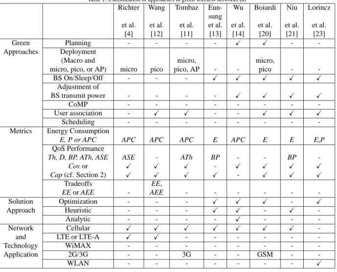
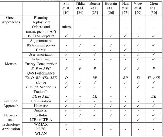
Tables 1 and 2 show a survey of recent papers that studied greening approaches and algorithms in wireless net-works, with focus on the metrics used for energy consumption and QoS performance.

Table 1: Classification of approaches in green wireless networks (a)

Richter Wang Tombaz Eun- Wu Boiardi Niu Lorincz sung

et al. et al. et al. et al. et al. et al. et al. et al. [4] [12] [11] [13] [14] [20] [21] [23]

Green Planning - - - - X X -

-Approaches Deployment

(Macro and micro, micro,

micro, pico, or AP) micro pico pico, AP - - pico -

-BS On/Sleep/Off - - - X X X X X Adjustment of BS transmit power - - - - X X X X CoMP - - - -User association - X X - - X X X Scheduling - - -

-Metrics Energy Consumption

E, P or APC APC APC APC E APC E E E,P

QoS Performance

Th, D, BP, ATh, ASE ASE - ATh BP - - BP

-Cov or X X X - X X X X Cap (cf. Section 2) X X X X - X X X Tradeoffs EE, EE or AEE - AEE - - - -Solution Optimization - - - X X X - X Approach Heuristic - - - X X _- X -Analytic - - - - X _{- -} -Network Cellular X X X X X X X

-and LTE or LTE-A X X - - -

-Technology WiMAX - - -

-Application 2G/3G - - 3G - - GSM -

-WLAN - - - X

4. Definitions and Notations

Let us introduce some definitions to formally characterize some concepts used in this article. The transmission delay of a given UE is defined as the inverse of the throughput perceived by this UE.

The peak rate of a given UE is defined as the throughput experienced by the UE when served alone in the cell. The peak rate of each UE depends on its received SNR from the serving BS. The latter depend on many factors such as the transmit power of the serving BS, the pathloss model, the bandwidth, etc.

Table 2: Classification of approaches in green wireless networks (b)

Son Yildiz Bousia Hossain Han Videv Chen et al. et al. et al. et al. et al. et al. et al. [10] [24] [25] [26] [27] [29] [30]

Green Planning - - -

-Approaches Deployment

(Macro and micro - - -

-micro, pico, or AP)

BS On/Sleep/Off X X X X X - X Adjustment of BS transmit power - X X X X X X CoMP - - - X X - -User association X X X - X X X Scheduling - - - X X

Metrics Energy Consumption

E, P or APC P P P - P P P

QoS Performance

Th, D, BP, ATh, ASE D - BP - BP Th Th, ASE

Cov or X X X - X X X Cap (cf. Section 2) X X - X - X X Tradeoffs EE or AEE - - EE - - EE Solution Optimization X - - - -Approach Heuristic X X X X X X X Analytic X - - - -Network Cellular X X X X X X X

and LTE or LTE-A - - - X X

Technology WiMAX X _{- - - - -}

-Application 2G/3G - - -

-WLAN - - -

-The coverage area of a given BS is defined as the geographical area where the received SNR of each UE is above a given minimum threshold. As the peak rate perceived by a given UE depends on its SNR, we thus consider that a UE is covered if it perceives a peak rate, from at least one BS, higher than a given peak rate threshold (χthreshold).

We consider a wireless access network with NbsBSs. we assume that each BS operates in two modes: active mode

and sleep mode. Nldenotes the number of transmit power levels of a BS. Transmitting at different power levels leads

to different coverage area sizes. The indexes i ∈ I = {1, . . . , Nbs}, and j ∈ J = {1, . . . , Nl}, are used throughout the

paper to designate a given BS and its transmit power level, respectively. Note that for j = 1, we consider that the BS transmits at the highest power level, and for j = Nl, the BS is in sleep mode. We term by k ∈ K = {1, . . . , Nu}, the

index of a given UE where Nuis the total number of UEs in the network. Let Ti, j,kdenote the transmission delay of UE

k associated with BS i transmitting at level j. Let χi, j,kdenote the peak rate perceived by UE k from BS i transmitting

at level j.

5. Multi-objective Optimization Formulation

Our approach is formulated as an optimization problem that consists of minimizing the power consumption of the network and the sum of the transmission delays of all UEs. A key tradeoff in our problem is between these two objectives. On the one hand, reducing the transmit power level of the BSs or switching them to sleep mode to save energy, may result in increasing the transmission delay. Precisely, if there are no coverage constraints, then all BSs could be in sleep mode, no UE is served, and the transmission delay becomes infinite. On the other hand, to minimize

the transmission delay, each BS should transmit at the highest power level possible. We thus formulate the joint Power-Delay minimization problem that enables tuning the predominance of each objective. The design variables in our Power-Delay minimization problem are as follows:

• The operation mode of the network BSs (on/sleep) and the corresponding transmit power level for active BSs. • The users association with the network BSs.

Let Λ be a matrix, with elements λi, j, defining the operation mode of the network BSs; and λi, jbe a binary variable

that indicates whether or not BS i transmits at level j.

λi, j=       

1 if BS i transmits at power level j, 0 otherwise.

Let Θ be a matrix, with elements θi,k, defining the users association with the network BSs; and θi,kbe a binary variable

that indicates whether or not a UE k is associated with BS i.

θi,k=        1 if UE k is associated with BS i, 0 otherwise.

The constraints on the decision variables are:

X j∈J λi, j=1, ∀i ∈ I, (1) X i∈I θi,k=1, ∀k ∈ K, (2)

λi,Nlθi,k=0, ∀i ∈ I, ∀k ∈ K, (3)

λi, j∈ {0, 1}, ∀i ∈ I, ∀ j ∈ J, (4)

θi,k∈ {0, 1}, ∀i ∈ I, ∀k ∈ K. (5)

Constraints (1) state that each BS transmits at only one power level. Constraints (2) ensure that a given UE is associ-ated with only one BS. In practice, when BSs are in sleep mode, some UEs will be out of coverage. Thus, to prevent UEs from being associated with a BS in sleep mode, we add constraints (3). These equations ensure that λi,Nland θi,k

are not both equal to one. Indeed, when BS i is in sleep mode, λi,Nlis equal to one, so θi,kof all UEs cannot be equal

to one. Constraints (4) and (5) are the integrality constraints for the decision variables λi, jand θi,k.

To eliminate some trivial cases that must not be included in the solution, we add the following constraints: • If UE k is not covered by BS i transmitting at the first (highest) power level, then

θi,k =0. (6)

The equation (6) prevents a given UE from being associated with a BS if that UE is not in the BS’s first power level coverage area.

• If UE k is not covered by BS i transmitting at power level j, j ∈ {2, .., Nl− 1}, then

λi, jθi,k=0, ∀ j ∈ {2, .., Nl− 1}. (7)

Equations (7) ensure that λi, jand θi,kare not both equal to one, which prevents a given UE from being associated

with a BS if the former is not in the BS’s jth_{power level coverage area.}

The goal of our approach is to jointly minimize the total network power and the total network delay. Thus, the two objectives are:

1. The total network power is defined as the total power consumption of active BSs in the network. pi, jdenotes

the average power consumed per BS i transmitting at power level j. Thus, the total network power, denoted by

Cp, is given by:

Cp(Λ) =

X

i∈I, j∈J

pi, jλi, j. (8)

The minimization of the total network power aims at reducing power consumption of the network.

2. The total network delay is defined as the sum of transmission delays (cf. Section 4) of all UEs in the network.

Ti, j,kbeing the transmission delay of UE k associated with BS i transmitting at level j, the total network delay,

denoted by Cd, is thus given by:

Cd(Λ, Θ) =

X

i∈I, j∈J, k∈K

Ti, j,kλi, jθi,k. (9)

The minimization of the total network delay aims at selecting the best user association that incurs the lowest sum of data unit transmission delays.

The proposed multi-objective optimization problem denoted by Multiobj-Power-Delay-Min aims at computing the transmit power level of the BSs deployed in the network as well as associating UEs with these BSs in a way that jointly minimizes the total network power and the total network delay. Therefore, Multiobj-Power-Delay-Min is given by: minimize Λ,Θ Cp(Λ), Cd(Λ, Θ), subject to (1) to (7). 6. Network Model

In this section, we investigate the problem of joint Power-Delay minimization for two types of networks. Firstly, we study the case of an IEEE 802.11g WLAN, where we consider a fair-rate sharing scheme because it is the resource sharing model that stems from the Carrier Sense Multiple Access (CSMA) protocol adopted in WLANs. Secondly, we study the case of an LTE network, where we consider the fair-time sharing scheme as it corresponds to the widely used OFDMA in LTE with a round robin scheduler.

6.1. Traffic and Delay Model

As the current downlink traffic on mobile networks is still several orders higher than the uplink traffic, we only consider the downlink traffic [31]. Moreover, elastic traffic currently constitutes the majority of Internet traffic [32, 33]. We thus consider an elastic traffic model. Furthermore, we assume that:

• The network is in a static state where users are stationary.

• The network is in a saturation state. A saturation state is a worst-case scenario where every BS has persistent traffic toward UEs.

• For the WLAN case, the inter-cell interference is mitigated by assigning adjacent WLAN BSs1_{to the different} IEEE 802.11 channels [34]. Particularly, in IEEE 802.11, the 2.4 GHz band consists of 14 overlapping channels, each occupying a bandwidth of 22 MHz. The three non-overlapping channels (channels 1, 6, and 11) are commonly used when designing a WLAN. Thus, one can assign one of these three frequencies to each network BS in a way that minimizes co-channel overlap. Assignment of frequencies is essentially a map coloring problem with three colors [35].

• In LTE networks, OFDMA is adopted as the downlink access method, which allows multiple UEs to transmit simultaneously on different subcarriers. As subcarriers are orthogonal, intra-cell interference is highly reduced. However, inter-cell interference is a key issue in OFDMA networks that greatly limits the network performance, especially for users located at the cell edge. One of the fundamental techniques to deal with the inter-cell interference problem is to control the use of frequencies over the various channels in the network [36]. There are three major frequency reuse patterns for mitigating inter-cell interference: hard frequency reuse (such as frequency reuse 1 and 3) , fractional frequency reuse and soft frequency reuse fractional [37]. Hard frequency reuse splits the system bandwidth into a number of distinct sub-bands according to a chosen reuse factor and neighboring cells transmit on different sub-bands. For instance, Frequency Reuse 3 scheme consists of dividing the frequency band into three sub-bands and allocating only one sub-band to a given cell, in such a way that the adjacent cells use different frequency bands. Compared with frequency reuse 1, this scheme leads to low interference with at the cost of a capacity loss because only one third of the resources are used in each cell [38].

6.1.1. Data Rate Model in IEEE 802.11 WLANs

With IEEE 802.11, neglecting the uplink traffic leads to a fair access scheme on the downlink channel. Accord-ingly, when a low-rate UE captures the channel, this UE will penalize the high-rate UEs. This also reduces the fair access strategy to a case of fair rate sharing of the radio channel among UEs [15] with the assumption of neglecting the 802.11 waiting times (i.e., DIFS2, SIFS3). Thus, all UEs will have the same mean throughput. When UE k is associated with BS i transmitting at level j, its mean throughput RW_{i, j,k}depends on its peak rate χi, j,kand the peak rates

of other UEs associated with this same BS (χi, j,k′,k′,k). RW

i, j,kis given by [7, 8]: RW_{i, j,k}= 1 1 χi, j,k + PNu k′=1,k′,k θi,k′ χi, j,k′ , (10)

where θi,k′is the binary variable indicating whether or not UE k′is associated with BS i.

6.1.2. Data Rate Model in LTE

In OFDMA, the system spectrum is divided into a number of consecutive orthogonal OFDM subcarriers. The Resource Block (RB) is the smallest resource unit that can be scheduled. The RB consists of 12 consecutive subcarriers for one slot (0.5 msec) in duration. In this paper, we consider a flat channel model where each UE has similar radio conditions on all the RBs. Moreover, we consider a fair-time sharing model where RBs are assigned with equal time to UEs within a given cell. These UEs are given the same chance to access the RBs. Based on these considerations and on UEs being stationary, the scheduler is equivalent to one that allocates periodically all RBs to each UE at each scheduling epoch. Hence, when UE k is associated with BS i transmitting at level j, its mean throughput R_{i, j,k}L depends on its peak rate χi, j,kand on the number of UEs associated with the same BS. RL_{i, j,k}is given by [8]:

RL_{i, j,k}= χi, j,k

1 +PNu

k′=1,k′,kθi,k′

, (11)

where θi,k′is the binary variable indicating whether or not UE k′is associated with BS i.

6.1.3. Delay Model in IEEE 802.11 WLANs and in LTE TW

i, j,kand T L

i, j,kdenote the transmission delay of UE k from BS i transmitting at level j in the case of a WLAN and

an LTE network, respectively. As mentioned in Section 4, the transmission delay for a given UE is the inverse of the throughput perceived by this UE. Thus, for the WLAN, TW

i, j,kis given by: T_{i, j,k}W = 1 χi, j,k + Nu X k′=1,k′,k θi,k′ χi, j,k′ , (12)

2_{DIFS: Distributed Coordination Function Interframe Space}

and for the LTE network, T_{i, j,k}L is given by: T_{i, j,k}L = 1 + PNu k′=1,k′,kθi,k′ χi, j,k . (13)

In fact, in our model, the transmission delay of a given user relies on the peak rate perceived by this user. The peak rate of each UE depends on its received SNR from the serving BS as mentioned in Section 4.

6.2. Power Consumption Model

6.2.1. Power Consumption Model in IEEE 802.11 WLANs

We consider the power consumption of an IEEE 802.11g WLAN, with BSs working in infrastructure mode. In practice, the transmission power of a WLAN BS is discrete and the maximum number of transmit power levels is equal to 5 or 6 depending on the BS manufacturer. Following the model proposed in [11], the power consumption of a WLAN BS is modeled as a linear function of the average transmit power:

pW_{i, j}=_{L (aπ}W

j +b), (14)

where pW i, jand π

W

j denote the average consumed power per WLAN BS i and the transmit power at level j respectively.

The coefficient a accounts for the power consumption that scales with the transmit power due to radio frequency amplifier and feeder losses. The coefficient b models the power consumed independently of the transmit power due to signal processing, power supply consumption and cooling. Recall that for j = 1, we consider that the BS transmits at the highest power level, and for j = Nl, the BS is in sleep mode. L reflects the activity level of the WLAN BSs. Since

we assume that the network is in a saturation state, L is equal to one; e.g., each active WLAN BS has at least one UE requesting data and to which all resources are being allocated [4, 11].

6.2.2. Power Consumption Model in LTE

Following the model proposed in the Energy Aware Radio and neTwork tecHnologies (EARTH) project [39], the power consumption of an LTE BS is also modeled as a linear function of the average transmit power:

∀i ∈ I, pL i, j=        NT RX(vπL_j +wj), 0 < πL_j ≤ PL₁, j = 1, . . . , (Nl− 1); NT RXwNl, π Nl j =0. (15) where p_{i, j}L and πL_j denote the average consumed power per LTE BS i and the transmit power at level j respectively. For j = 1, we consider that the BS transmits at the highest power level, and for j = Nl, the BS is in sleep mode. The

coefficient v is the slope of the load-dependent power consumption and it accounts for the power consumption that scales with the transmit power due to radio frequency amplifier and feeder losses. The coefficients wj( j = 1, .., (Nl−

1)) represent the power consumption at zero output power (it is actually estimated using the power consumption calculated at a reasonably low output power, assumed to be 1% of pL

1). These coefficients model the power consumed independently of the transmit power due to signal processing, power supply consumption and cooling. wNl is a

coefficient that represents the sleep mode power consumption. NT RXis the number of BS transceivers. 7. Optimization Approach in WLANs and LTE Scenarios

In this section we present the multi-objective optimization approach for WLANs and LTE cases. For WLANs, the proposed multi-objective optimization problem denoted by Multiobj-Power-Delay-Min-WLAN is thus obtained from the problem Multiobj-Power-Delay-Min by replacing pi, j and Ti, j,k by the expressions of pW_{i, j} and T_{i, j,k}W . Let

CW_p and CW_d denote the total network power and the total network delay for this case, respectively. Therefore, the Multiobj-Power-Delay-Min-WLAN problem is given by:

minimize Λ,Θ C W p(Λ) = X i∈I, j∈J (aπW_j +_{b) λi, j, (16)} C_dW(Λ, Θ) = X i∈I, j∈J,k∈K (λi, jθi,k χi, j,k + Nu X k′=1,k′,k λi, jθi,kθi,k′ χi, j,k′ ), (17) subject to: (1) to (7).

For LTE, the proposed multi-objective optimization problem denoted by Multiobj-Power-Delay-Min-LTE is thus obtained from the problem Multiobj-Power-Delay-Min by replacing pi, jand Ti, j,kby the expressions of pLi, jand T

L i, j,k.

Let CL

pand CdLdenote the total network power and the total network delay for this case, respectively. Therefore, the

Multiobj-Power-Delay-Min-LTE problem is given by: minimize Λ,Θ C L p(Λ) = X i∈I, j∈J NT RX(vπLj+wj) λi, j, (18) C_dL(Λ, Θ) = X i∈I, j∈J,k∈K

λi, jθi,k+ PN_k′u=1,k′,kλi, jθi,kθi,k′

χi, j,k

, (19)

subject to: (1) to (7).

8. From Multi-objective Optimization to Single-objective Optimization

Solving a multi-objective optimization problem is a very challenging task. In this section, we provide two solu-tion methods to multi-objective optimizasolu-tion: the ǫ-constraints method and the weighted sum method. Using these techniques, we obtain new optimization problems with a single objective function, which are easier to solve than the original problems.

8.1. ǫ-Constraint Method

The ǫ-constraint method is based on minimizing one objective function and considering the other objectives as constraints bound by some allowable level ǫn. Hence, a single objective minimization is carried out subject to

addi-tional constraints on the other objective functions. In our multi-objective optimization, since we have two objective functions, this method may be formulated in two variants presented in the following.

Power Minimization subject to Delay Constraints problem. The power minimization subject to delay constraints

problem, denoted by Power-Min-Delay-Const, is given by: minimize

Λ Cp(Λ), (20)

Cd(Λ, Θ) ≤ ǫ1, (21)

subject to: (1) to (7).

ǫ1is a value of the total network delay which we do not wish to exceed. The Power-Min-Delay-Const problem can be literally expressed as: given some delay bound (constraint (21)), is there a BS operation mode and a user association satisfying constraints (1) to (7) such that the total network power Cpis minimized?

Delay Minimization subject to Power Constraints problem. The delay minimization subject to power constraints

problem, denoted by Delay-Min-Power-Const is given by: minimize

Λ,Θ Cd(Λ, Θ), (22)

Cp(Λ) ≤ ǫ2, (23)

subject to: (1) to (7).

ǫ2is a value of the total network power which we do not wish to exceed. In other words, the aforementioned problem can be expressed as: given some power bound (constraint (23)), is there a BS operation mode and a user association satisfying constraints (1) to (7) such that the total network delay is Cdis minimized?

The major drawback of such problems is that the decision maker (i.e, the network operator) cannot estimate the total network delay or the total network power. Thus, it is hard to choose the adequate bounds on the delay or the power.

8.2. Weighted Sum Method

The weighted sum method consists of summing the objective functions combined with different weighting co-efficients. The multi-objective optimization problem is transformed into a scalar optimization problem, denoted by Weighted-Sum-Power-Delay-Min: minimize Λ,Θ Ct(Λ, Θ) = αCp(Λ) + ββ ′ Cd(Λ, Θ), (24) subject to: (1) to (7).

where Ctdenotes the total network cost defined as the weighted sum of the total network power and the total network

delay. β′_{is a normalization factor that will scale the two objectives properly. α and β are the weighting coefficients} representing the relative importance of the two objectives. It is usually assumed that α + β = 1 and that α and β ∈ [0,1]. In particular, when α equals 1 and β equals 0, we only focus on the power saving. As α decreases and β increases more importance is given to minimizing the delay. By tuning the weighting coefficients, we obtain different points located on the Pareto frontier presenting all the compromises between the two objectives. The weighting coefficients are also called tuning factors, as decision makers use them to fine-tune the model to reflect their decision preferences. In this article, we choose the weighted sum method in order to study the tradeoffs between minimizing the power consumption of the network and minimizing the sum of UE transmission delays in the network for the WLAN and LTE cases. Let Weighted-Sum-Power-Delay-Min-WLAN and Weighted-Sum-Power-Delay-Min-LTE denote the scalar optimization problems for the considered cases, respectively. Consequently, the objective functions of these problems are obtained by replacing Cp and Cd by CWp and CdW for the WLAN case and by C

L

p and CdL for the LTE case,

respectively. Let CW

t and CtLdenote the total network cost for WLAN and LTE cases, respectively.

Therefore, the objective function of the Weighted-Sum-Power-Delay-Min-WLAN problem is given by:

minimize Λ,Θ C W t (Λ, Θ) = α X i∈I, j∈J (aπW_j +_{b) λi, j}+_ββ′ X i∈I, j∈J,k∈K (λi, jθi,k χi, j,k + Nu X k′=1,k′,k λi, jθi,kθi,k′ χi, j,k′ ); (25)

and the objective function of the Weighted-Sum-Power-Delay-Min-LTE problem is given by:

minimize Λ,Θ C L t(Λ, Θ) = α X i∈I, j∈J NT RX(vπLj +wj) λi, j+ββ′ X i∈I, j∈J,k∈K

λi, jθi,k+ PN_k′u=1,k′,kλi, jθi,kθi,k′

χi, j,k

. (26)

The scalar optimization problems are binary non-linear. Such problems can be optimally solved using an exhaustive search algorithm [40]. However, the complexity of searching only for the operation mode of the BS is in O(NNbs

l ). This

makes the exhaustive search very computational intensive, and rapidly becomes intractable for modest sized networks. Thus, in the next section we convert the optimization problems into MILP problems to make them computationally tractable.

9. Mixed Integer Linear Programming Formulation

In this section, we explain how to convert our non-linear optimization problems Weighted-Sum-Power-Delay-Min-WLAN and Weighted-Sum-Power-Delay-Min-LTE into MILP problems. A MILP problem consists of a linear objective function, a set of linear equality and inequality constraints and a set of variables with integer restrictions. The number of constraints and variables are important factors when estimating if a problem is tractable. Generally, MILP problems are solved using a linear-programming based branch-and-bound approach. The idea of this approach is to solve Linear Program (LP) relaxations of the MILP and to look for an integer solution by branching and bounding on the decision variables provided by the LP relaxations. Thus, in a branch-and-bound approach the number of integer variables determines the size of the search tree and influences the running time of the algorithm.

Based on our work [41], to linearize the non-linear optimization problems we replace the non-linear terms by new variables and additional inequality constraints which ensure that the new variables behave according to the non-linear

terms they are replacing. Particularly, in the objective functions ((25) and (26)), we replace each quadratic term λi, jθi,k

by a new linear variable yi, j,kand add the following three inequalities to the set of constraints:

yi, j,k− λi, j≤ 0, ∀i ∈ I, ∀ j ∈ J, ∀k ∈ K, (27)

yi, j,k− θi,k≤ 0, ∀i ∈ I, ∀ j ∈ J, ∀k ∈ K, (28)

λi, j+θi,k− yi, j,k≤ 1, ∀i ∈ I, ∀ j ∈ J, ∀k ∈ K. (29)

The inequalities (27) and (28) ensure that yi, j,kequals zero when either λi, jor θi,k equals zero, while the inequalities

(29) force yi, j,k to be equal to one if both λi, j and θi,kequal one. Moreover, constraints (3) and (7) will be replaced

respectively by (30) and (31):

yi,Nl,k=0, ∀i ∈ I, ∀k ∈ K, (30)

yi, j,k=0, ∀i ∈ I, ∀ j ∈ {2, .., Nl− 1}, ∀k ∈ K/χi, j,k≤ χthreshold. (31)

Similarly, we replace each term λi, jθi,kθi,k′in the objective functions ((25) and (26)) by a new variable z_{i, j,k,k}′and add

the following inequalities to the set of constraints:

zi, j,k,k′− λ_{i, j}≤ 0, ∀i ∈ I, ∀ j ∈ J, ∀k < k′∈ K, (32)

zi, j,k,k′− θ_i,k≤ 0, ∀i ∈ I, ∀ j ∈ J, ∀k < k′∈ K, (33)

zi, j,k,k′− θ_i,k′ ≤ 0, ∀i ∈ I, ∀ j ∈ J, ∀k < k′∈ K, (34)

λi, j+θi,k+θi,k′− z_{i, j,k,k}′≤ 2, ∀i ∈ I, ∀ j ∈ J, ∀k < k′∈ K, (35)

zi, j,k,k′− z_{i, j,k}′_,k=0, ∀i ∈ I, ∀ j ∈ J, ∀k < k′∈ K. (36)

The inequalities (32), (33) and (34) ensure that zi, j,k,k′ is equal to zero when either λ_{i, j} or θ_i,k or θ_i,k′ equals zero,

while the inequalities (35) force yi, j,k to be equal to one if λi, j, θi,k and θi,k′ are equal to one. Furthermore, as

λi, j θi,k θi,k′ = λ_{i, j} θ_i,k′ θ_i,k, constraints (36) force z_{i, j,k,k}′ to be equal to z_{i, j,k}′_,k. In addition, we give the bound

con-straints for the variables yi, j,kand zi, j,k,k′as follows:

0 ≤ yi, j,k≤ 1, ∀i ∈ I, ∀ j ∈ J, ∀k ∈ K, (37)

0 ≤ zi, j,k,k′ ≤ 1, ∀i ∈ I, ∀ j ∈ J, ∀k < k′∈ K. (38)

The MILP Weighted-Sum-Power-Delay-Min-WLAN problem is given by: minimize Λ,Y,Z C W t (Λ, Y, Z) = α X i∈I, j∈J (aπW_j +_{b) λi, j}+_ββ′ X i∈I, j∈J,k∈K (yi, j,k χi, j,k + X k′_∈K,k′,k zi, j,k,k′ χi, j,k′ ), (39)

subject to: (1) to (7) and (27) to (38);

where yi, j,k and zi, j,k,k′ are respectively the elements of the matrices Y and Z. Similarly, the MILP

Weighted-Sum-Power-Delay-Min-LTE problem is given by: minimize Λ,Y,Z C L t(Λ, Y, Z) = α X i∈I, j∈J (NT RX(vπLj+wj)) λi, j+ββ′ X i∈I, j∈J,k∈K (yi, j,k + P_k′_∈K,k′,kzi, j,k,k′ χi, j,k ), (40) subject to: (1) and (2), (4) to (6), and (27) to (38);

Table 3: Notation Summary Notation Definition

I Set of network BSs

J Set of transmit power levels of a given BS

K Set of UEs in the network

Nbs The total number of BSs

Nl The total number of transmit power levels

Nu The total number of UEs

pi, j The average consumed power per BS i transmitting at power level j

πL

j The transmit power at level j for LTE BSs

πW

j The transmit power at level j for WLAN BSs

χi, j,k The peak rate perceived by UE k from BS i transmitting at level j

Ti, j,k The transmission delay of UE k associated with BS i transmitting at level j

θi,k A binary variable that indicates if UE k is associated with BS i

λi, j A binary variable that indicates if BS i transmits at power level j

yi, j,k A real variable that indicates if UE k is associated with BS i

transmitting at power level j

zi, j,k,k′ A real variable that indicates if UE k and UE k′are associated with BS i

transmitting at power level j

Table 4: Five studied settings for WLAN and LTE scenarios

Settings Weighting coefficients value Description

S1 α= 0.99, β=0.01 Preference is given to saving power S2 α= 0.75, β=0.25

S3 α= 0.5, β=0.5 Balance the tradeoff between minimizing power and delay S4 α= 0.25, β=0.75

S5 α= 0.01, β=0.99 Preference is given to minimizing delay

10. Performance Evaluation

To study the tradeoff between minimizing the power consumption of the network and minimizing the sum of UE transmission delays in the network, we tune the values of the weights α and β (in (39) and (40)) associated with the total network power and total network delay respectively, and investigate the obtained solutions for WLANs and LTE networks. We consider five settings illustrated in Table 4. Settings S1 and S2 match the case where preference is given to power saving. Setting S3 matches the case where the power and delay are equally important. Settings S4 and S5 match the case where preference is given to minimizing delay.

Moreover, the normalization factor β′_{is calculated in each simulation so as to scale the total network power and the} total network delay [42]. Furthermore, we adopt the Monte Carlo method by generating 50 snapshots with different random uniform UE distribution. After doing the calculations for all the snapshots, we provide the 95% Confidence Interval (CI) for each simulation result. In the simulation results, the optimal solutions are provided for the different settings (S1, S2, S3, S4, S5).

10.1. Power and User Association Reference Models

In legacy WLANs or cellular networks, BSs transmit at a fixed power level, and UEs are associated with the BS delivering the highest SNR [12, 43]. Based on these legacy networks, we devise a reference model composed of i) the Highest Power Level (HPL) as the reference power model, which assumes that all BSs transmit at the highest power level, and ii) the Power-based User Association (Po-UA) as the reference user association model, which associates a UE with the BS where it obtains the highest SNR. In what follows, we denote the reference model by Po-UA/HPL. The total network power and the total network delay of this model will serve as reference values for comparison of

Table 5: Covering BSs per UE vs. inter-cell distance in WLAN scenarios.

Inter-cell distance [m] 120.8 134.2 147.6 161.1 174.5 187.9 201.3 214.8

Number of covering BSs per UE 2.02 1.76 1.53 1.38 1.25 1.15 1.05 1.00

the results. In the following, we present the evaluation method and the simulation results for the WLAN and LTE scenarios.

10.2. IEEE 802.11g WLAN Scenarios 10.2.1. Evaluation Method

To evaluate the tradeoff between power and delay in WLANs, we compute the optimal solution of our MILP Weighted-Sum-Power-Delay-Min-WLAN problem with the GLPK (GNU Linear Programming Kit) solver [44] over a network topology composed of nine cells (Nbs =9) using the IEEE 802.11g technology and six UEs in each cell

(Nu=9 ∗ 6 = 54). The positioning of the WLAN BSs in the network is performed following a grid structure and the

positioning of UEs is generated randomly following a uniform distribution.

In the BS power model, for simplicity, we set the number of transmit power levels to three (Nl=3). Precisely,

an active BS is able to transmit at two different power levels, and when the power level equals Nl =3, the BS is in

sleep mode. For the WLAN, we consider that when the BS is in sleep mode, it consumes only power due to signal processing neglecting the cooling. It is estimated that the power consumption of signal processing circuits accounts for only 10% of the total consumed power [45]. Therefore, we assume that in sleep mode, the WLAN BS power consumption is negligible, and it is considered to be switched-off. We aim to compute the optimal solution of the MILP problem. Thus, if we increase Nl, the granularity will be finer but the problem becomes intractable. The input

parameters of the power consumption model in (14) are as follows: i) as proposed in [11], the values of a and b used in this paper are a = 3.2 and b = 10.2; ii) as proposed in [46], the transmit power at levels one and two is πW

1 = 0.03 W and πW

2 = 0.015 W, respectively. Hence, the average power consumed per BS i ∈ I at the first, second and third power levels is given by pi,1= 10.296 W, pi,2= 10.248 W, and pi,3=0, respectively.

Peak rate and coverage area computation. In NS2 [47], we implement a benchmark scenario that enables the

com-putation of the peak rate perceived by the UE from the BS and the coverage area of the WLAN BS. Particularly, the benchmark scenario consists of a free propagation model to characterize the WLAN radio environment, an IEEE 8021.11g BS working at 2.4 GHz, and a single UE at different positions. This UE receives Constant Bit Rate (CBR) traffic from the BS with a packet size of 1000 bytes and an inter-arrival time of 0.4 ms corresponding to a rate of 20 Mbit/s. This leads to a saturation state of the network according to the assumption presented in section 6.1. In these conditions, the throughput experienced by the single UE is the maximum achievable throughput (peak rate) for the current SNR. We run this scenario for each BS transmit power level (π1 = 0.03 W and π2 = 0.015 W) to obtain

χi,1,k and χi,2,k, respectively, for the corresponding UE. Figure 2 shows the peak rate perceived by the UE from the

BS, transmitting at the first and the second power level, as a function of the distance. In addition, the coverage ra-dius for the first and second power levels are R1 = 107,4 m and R2= 75,8 m, respectively. These radii correspond to an SNR threshold that equals -0.5 dB at the cell boundary. This SNR is the minimum value to be maintained in order to consider that a given UE is covered by a BS. It corresponds to a cell edge peak rate that equals 1 Mbit/s

(χthreshold=1 Mbit/s) on the downlink. We note that, considering a more realistic propagation model will only affect

the values of the user peak rate. The considered peak rate will be lower than that considering a Free propagation model.

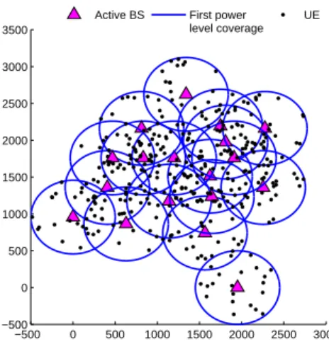
In the following, the simulation results are plotted as a function of the inter-cell distance D. Particularly, this parameter has a large impact on not only the computational complexity of the algorithm but also on the quality of the solution. For small inter-cell distances, we obtain a dense coverage area, while large inter-cell distances produce a sparse coverage area. Table 5 shows the average number of covering BSs per UE as a function of the inter-cell distance. For D = 120.8 m, we obtain a dense coverage area where the average number of covering BSs per UE is 2.02. As D increases, the average number of covering BSs per UE decreases to be equal to one when there is no overlap between cells (D = 2R1). Figure 3 shows an example of the network topology with an inter-cell distance equals 120.8 m.

0 10 20 30 40 50 60 70 80 90 100 110 0 2 4 6 8 10 12 14 16 18 20 Distance [m] Peak rate [Mb/s] π₁ = 30 mW π₂ = 15 mW

Figure 2: Peak rates in IEEE 802.11g for different transmit power levels. Active BS First power level coverage Second power level coverage UE

Figure 3: An example of WLAN topology with inter-cell distance

D = 120.8 m. 100 120 140 160 180 200 220 −5 0 5 10 15 20 Inter−cell distance [m]

Percentage of power saving [%]

S1 (α=0.99 β=0.01) S2 (α=0.75 β=0.25) S3 (α=β=0.5) S4 (α=0.25 β=0.75) S5 (α=0.01 β=0.99)

Figure 4: Power saving for the considered settings in WLAN sce-narios. 100 120 140 160 180 200 220 6.5 7 7.5 8 8.5 9 9.5 10 10.5 11 11.5x 10 −5 Inter−cell distance [m]

Total network delay [s]

Po−UA/HPL S1 (α=0.99 β=0.01) S2 (α=0.75 β=0.25) S3 (α=β=0.5) S4 (α=0.25 β=0.75) S5 (α=0.01 β=0.99)

Figure 5: Total network delay for the considered settings and for Po-UA/HPL in WLAN scenarios.

10.2.2. Simulation Results

Let us start by examining the power saving achieved for the five considered settings, which is computed as follows: 100 × (1 −total network power for the considered setting

total network power for Po-UA/HPL model ), (41) where the total network power is computed according to the value of CW

p in (16). Recall that in the Po-UA/HPL

reference model, all BSs transmit at the highest power level.

Figure 4 plots the percentage of power saving for the five considered settings as a function of the inter-cell distance

D. S1 and S2 have the highest percentage of power saving, followed successively by S3 then S4 for D ranging from

120.8 m to 161.1 m, while no power saving is obtained for D ≥ 161.1 m. For instance, when D = 120.8 m, we obtain power saving of up to 16% in S1 and S2, followed by S3 at 12.22% and by S4 at 1.33%. S5 has no power saving for any distance. In other words, in S5, we obtain a BS operation mode where all BSs transmit at the highest power level (similar to the Po-UA/HPL model). Precisely, in this setting preference is given to minimizing the sum of UE delays, so when all BSs transmit at the highest level, UEs experience lower delays in comparison with the case where some of the BSs transmit at the second power level or are switched off.

In order to examine the cause of significant power savings in settings S1, S2 and S3, we plot Fig. 6, which illustrates the percentage of the BS operation modes for D ranging from 120.8 m to 161.1 m. We see that S1 has the highest percentages of BSs transmitting at the second power level and switched-off, followed by S2 then by S3 for the different values of D. Moreover, for these three settings, we note that when D increases, the percentage of

120.8 134.2 147.6 161.1 0 20 40 60 80 100 120 Inter−cell distance [m] BS operation modes [%]

First power level Second power level Switched−off (a) S1 (α=0.99 β=0.01) 120.8 134.2 147.6 161.1 0 20 40 60 80 100 120 Inter−cell distance [m] BS operation modes [%]

First power level Second power level Switched−off (b) S2 (α=0.75 β=0.25) 120.8 134.2 147.6 161.1 0 20 40 60 80 100 120 Inter−cell distance [m] BS operation modes [%]

First power level Second power level Switched−off

(c) S3 (α=0.5 β=0.5) Figure 6: Percentage of BS operation modes in settings S1, S2 and S3 in WLAN scenarios.

switched-off BSs decreases, and the percentage of BSs transmitting at the second power level increases. On the one hand, this explains the decreasing curves for the corresponding inter-cell distances in Fig. 4. On the other hand, for low values of D (i.e., 120.8 m), this behavior is due to the relatively high number of covering BSs per UE (i.e., 2.02 as shown in Tab. 5). Thus, the possibility of switching off the BS or transmitting at low power level is high. However, for large D values, the number of covering BSs per UE decreases, and thus the possibility to switch off a BS or to transmit at low power level decreases due to the coverage constraints.

We now investigate the total network delay for the considered settings compared to the Po-UA/HPL model while varying the inter-cell distance (D). The total network delay is computed according to the value of CW_d in (17). For the comparison of the five settings, Fig. 5 shows that S5 has the lowest total network delay, followed successively by S4, S3, S2, and finally S1. Particularly, in S5, more weight is given to minimizing the delay (β=0.99), thus we obtain a network operation mode where all BSs transmit at the highest power level (as shown in Fig. 4). The problem becomes a user association problem that aims to minimize the sum of network UE transmission delays. With the decrease of β, more BSs are switched off or transmit at the second power level (as shown in Fig. 6), and thereby UEs will experience higher delay. Compared to the Po-UA/HPL model, we obtain a delay reduction for all the inter-cell distances in S4 and S5. For instance, the delay reduction is 4.5% and 6.64% in S4 and S5, respectively, for D=120.8 m. However, we obtain a higher total network delay compared to Po-UA/HPL for all D in S1, S2 and S3. Further, we see that in S4 and S5, the total network delay has an increasing curve. Precisely, for a given UE distribution, when D increases, the SNR of the UE will decrease, causing the delay to increase. Similarly, we also see that in S2 and S3, the total network delay has an increasing curve but with lower slope at the first inter-cell distances. In S1, the total network delay has a decreasing curve for D between 120.8 m and 161.1 m and then it increases for D ≥ 161.1 m. In particular, for D between 120.8 m and 161.1 m, more BSs transmit at either the highest power level or the second power level (Fig. 6(a)). UEs will thereby experience a lower delay. Note that all the curves converge to the same point. Indeed, when

D increases, the cell overlap decreases, and thus, the optimal solution for the five settings turns on the BSs to achieve

a point where all the BSs transmit at the highest power level. Therefore, the problem boils down to a user association problem that minimizes the sum of UE delays.

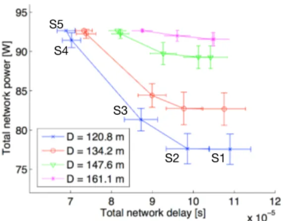
In Fig. 7, we plot the power-delay tradeoff curves for different inter-cell distances D ranging from 120.8 m to 161.1 m. The five points of the illustrated curves are obtained by plotting the values of the 95% CI of the total network power as a function of the 95% CI of the total network delay for the five considered settings. For all the inter-cell distances, we obtain a reduction in the network power consumption at the cost of delay increase. In particular, for D=120.8 m, in S5 (α = 0.01 β=0.99), we obtain the solution with the lowest total network delay (6.88 × 10−5_s) and the highest total network power (92.664 Watt); while in S1 (α = 0.99 β=0.01), we obtain the solution with the lowest total network power (77.62 W) and the highest total network delay (10.90 × 10−5_{s). Moreover, we note that} when D increases, the tradeoff curves become flat. For instance, for D=161.1 m, we obtain similar total network power in the five settings. Indeed, for sparse coverage area, the problem in the five settings becomes similar to a user association problem where there is no longer an interesting power-delay tradeoff. In fact, these curves represent the Pareto frontier at different inter-cell distances. Hence, a network operator has the option to choose the operation point of the network. For instance, the operator can choose the optimal inter-cell distance of his network. Moreover, the operator has the choice to privilege power saving, minimize delay, or balance the tradeoff between the two objectives.

S1 S2 S3

S4 S5

Figure 7: Pareto frontier at different inter-cell distances in WLAN scenarios.

10.3. Computational complexity

In order to assess the computational complexity of the optimal solution, we calculate in the following its compu-tation time and the number of binary integer variables. Also, we compute the number of non-zero elements of the matrix defining the constraints of the minimization problem. Figure 8 shows the 95% CI of the computational

com-120.8 134.2 147.6 161.1 0 200 400 600 800 1000 1200 1400 1600 Inter−cell distance [m] Computation time [s]

(a) Computation time of the optimal solution

120.8 134.2 147.6 161.1 0 20 40 60 80 100 120 Inter−cell distance [m] Integer variables

(b) Number of binary integer variables

120.8 134.2 147.6 161.1 0 0.5 1 1.5 2x 10 4 Inter−cell distance [m]

Non zero elements

(c) Number of non-zero elements Figure 8: Optimal solution computational complexity measurements.

plexity measurements as a function of the inter-cell distance (D). We note that the computation time of the optimal solution decreases when D increases as shown in Fig. 8(a). Precisely, when D increases, the number of binary integer variables and non-zero elements decreases as shown in Fig. 8(b) and Fig. 8(c). In fact, when the inter-cell distance increases, the number of UEs covered by each BS decreases. This causes the related solution space (for selecting the BS transmit power level, and the user association) to be small. Thereby, this decreases the number of binary integer variables and non-zero elements. Moreover, we note that we cannot obtain solutions for very dense networks (e.g.,

D ≤ 120.8 m), as the problem becomes intractable. Therefore, in order to overcome such issue, we introduce in [16] a

heuristic algorithm that computes satisfactory solutions for the problem while keeping low computation complexity.

10.4. LTE Scenario 10.4.1. Evaluation Method

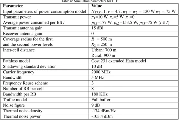
To evaluate the tradeoff between power and delay in LTE, we compute the optimal solution of our MILP Weighted-Sum-Power-Delay-Min-LTE problem using the CPLEX solver [48]. The input data for the CPLEX solver are gen-erated using MATLAB [49]. Thus, in MATLAB, we implement an LTE network topology where the LTE BSs are transmitting using omni-directional antennas in three deployment cases: urban, rural and realistic LTE deployment. For both cases (urban and rural deployment), the network topology is composed of nine cells (Nbs=9) and the