Discrete Controller Synthesis for Infinite State Systems with ReaX

Motivated by recent work of Au, C´ ebron, Dahlqvist, Gabriel, and Male, we study regularity properties of the distribution of a sum of two selfad- joint random variables in a

Ainsi qu’il a ´et´e rappel´e en introduction, les ´etoiles `a neutrons sont des astres tr`es relativistes, presque autant que les trous noirs, leur param`etre de relativit´e

is a curve germ then it is in fact bilipschitz equivalent to the metric cone over its link with respect to the inner metric, while the data of its Lipschitz outer geometry is

Patients #18, 20 and 23 had negative FDG- PET examinations at baseline (cf. text for further discussion); b Semiquantitative grading of intensity of 18-F-Fluorodeoxyglu- cose

For the present test assessment, we used different groups of animals or sera to evaluate the operating characteristics: Experimentally infected calves served to comparatively

The purpose of this study was to assess the motor output capabilities of SMA, relative to M1, in terms of the sign (excitatory or inhibitory), latency and strength of

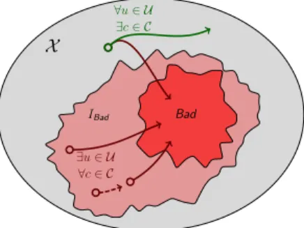
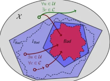
Our aim is to modify the initial system so that the controlled system could not enter the states of E(v). However, it is not possible to perform this transformation on the

Physical intuition tells us that a quantum system with an infinite dimen- sional Hilbert space can be approximated in a finite dimensional one if the amount of energy transferred

REFERENCES

Benveniste, A., Caspi, P., Edwards, S., Halbwachs, N., Le Guernic, P., and de Simone, R. (2003). The Syn-chronous Languages Twelve Years Later. Proceedings of the IEEE, 91(1), 64–83.
Billon, J. (1987). Perfect normal forms for discrete programs. Technical report, Bull.
Cassandras, C. and Lafortune, S. (2007). Introduction to Discrete Event Systems. Springer.
Cassez, F., David, A., Fleury, E., Larsen, K., and Lime, D. (2005). Efficient on-the-fly algorithms for the analysis
of timed games. In Conf. on Concurrency Theory (CONCUR), volume 3653 of LNCS, 66–80.
Clarke, E.M., McMillan, K.L., Zhao, X., Fujita, M., and Yang, J. (1993). Spectral transforms for large boolean functions with applications to technology mapping. In 30th Conference on Design Automation, 54–60. IEEE. Cousot, P. and Cousot, R. (1976). Static determination
of dynamic properties of programs. In Proceedings of the Second International Symposium on Programming, 106–130. Dunod, Paris, France.
Cousot, P. and Cousot, R. (1977). Abstract interpretation: a unified lattice model for static analysis of programs by construction or approximation of fixpoints. In Proceedings of the 4th ACM Symposium on Principles of Programming Languages, POPL ’77, 238–252. Cousot, P. and Cousot, R. (1979). Systematic design of
program analysis frameworks. In Proceedings of the 6th ACM SIGACT-SIGPLAN Symposium on Principles of Programming Languages, POPL ’79, 269–282.
Cousot, P. and Halbwachs, N. (1978). Automatic discovery of linear restraints among variables of a program. In Proceedings of the 5th ACM Symposium on Principles of Programming Languages, POPL ’78, 84–96.
Delaval, G., Marchand, H., and Rutten, E. (2010). Con-tracts for modular discrete controller synthesis. In Proceedings of the Conference on Languages, Compilers, and Tools for Embedded Systems, 57–66.
Delaval, G., Rutten, E., and Marchand, H. (2013). Inte-grating discrete controller synthesis into a reactive pro-gramming language compiler. Discrete Event Dynamic Systems, 23(4), 385–418.
Halbwachs, N., Proy, Y.E., and Roumanoff, P. (1997). Verification of Real-Time Systems using Linear Relation Analysis. Form. Methods Syst. Des., 11, 157–185. Holloway, L., Krogh, B., and Giua, A. (1997). A survey
of Petri net methods for controlled discrete event sys-tems. Discrete Event Dynamic Systems: Theory and Application, 7, 151–190.
Jeannet, B. (2003). Dynamic Partitioning in Linear Relation Analysis: Application to the Verification of Reactive Systems. Form. Methods Syst. Des., 23, 5–37. Jeannet, B. and Min´e, A. (2009). Apron: A library of numerical abstract domains for static analysis. In Computer Aided Verification, 661–667. Springer. Kalyon, G., Le Gall, T., Marchand, H., and Massart, T.
(2011). Symbolic supervisory control of infinite transition systems under partial observation using abstract inter-pretation. Discrete Event Dynamic Systems : Theory and Applications, 22(2), 121–161.
Kumar, R., Garg, V., and Marcus, S. (1993). Predicates and predicate transformers for supervisory control of discrete event dynamical systems. IEEE Trans. Autom. Control, 38(2), 232–247.
Kumar, R. and Garg, V. (2005). On computation of state avoidance control for infinite state systems in assignment program model. IEEE Trans. on Automation Science and Engineering, 2(2), 87–91.
Le Gall, T., Jeannet, B., and Marchand, H. (2005). Supervisory control of infinite symbolic systems using abstract interpretation. In Proceedings of the 44th IEEE Conference on Decision and Control, 31–35.
Li, Y. and Wohnam, W. (1994). Control of vector discrete-event systems-part ii : controller synthesis. IEEE Trans. Automatic Control, 39(3), 512–531.
Marchand, H., Bournai, P., Le Borgne, M., and Le Guernic, P. (2000). Synthesis of discrete-event controllers based on the signal environment. Discrete Event Dynamic System: Theory and Applications, 10(4), 325–346.
Marchand, H. and Samaan, M. (2000). Incremental Design of a Power Transformer Station Controller Using a Controller Synthesis Methodology. IEEE Trans. Softw. Eng., 26, 729–741.
Miremadi, S., Akesson, K., and Lennartson, B. (2008). Extraction and representation of a supervisor using guards in extended finite automata. In 9th International Workshop on Discrete Event Systems, 193–199.
Ramadge, P.J. and Wonham, W.M. (1989). The control of discrete event systems. Proceedings of the IEEE; Special issue on Dynamics of Discrete Event Systems, 77(1), 81–98.
Schrammel, P. (2013). Logico-Numerical Verification Methods for Discrete and Hybrid Systems. Ph.D. thesis, University of Grenoble.
Schrammel, P. and Jeannet, B. (2012). Applying Abstract Acceleration to (Co-)Reachability Analysis of Reactive Programs. J. Symb. Comput., 47(12), 1512–1532.
Figure
Fig. 1. Exact computation of the forbidden states I Bad . 2.2 Control of an ASTS: Boolean Case
Fig. 2. Over-approximation I Bad ′ of the possibly non- non-computable set of forbidden states I Bad .
Fig. 4. Synthesis times for the parallel tasks example.