Frequency analysis of daily maximum temperature in southern Québec with a view to interpret heatwaves = Analyse frequentielle des températures maximum journalières du sud du Québec pour des fins d'interprétation des canicules.

(1)

FREQUENCY ANALYSIS OFDAILY

MAXIMUM TEMPERATURE IN

SOUTHERN QUÉBEC WITH A VIEW

TO INTERPRET HEATW A VES

(2)

(3)

c-~

C>UR4,..,C>S

FREQUENCY ANAL YSIS OF DAIL Y MAXIMUM

TEMPERATURE IN SOUTHERN QUÉBEC WITH A

VIEW TO INTERPRET HEATW A VES

ANALYSE FREQUENTIELLE DES TEMPÉRATURES

MAXIMUM JOURNALIÈRES DU SUD DU QUÉBEC POUR

DES FINS D'INTERPRÉTATION DES CANICULES

Rapport présenté au Groupe Impacts et Adaptations du Consortium Ouranos Par

M. Naveed Khaliq

André St-hilaire

Taha B.M.]. Ouarda

Bernard Bobée

AOUT 2004

(4)

Référence

Khaliq, M.N., A. St-Hilaire, T.B.M.J. Ouarda, B. Bobée. 2004. Frequency Analysis of daily maximum temperature in southem Québec with a view to interpret heatwaves. INRS-ETE, Research Report R-747, 34 pages and 3 appendices.

(5)

LIST OF TABLES

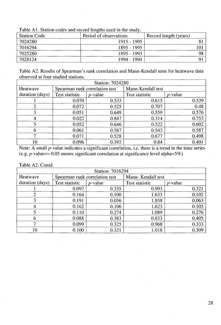
Table No. and Caption ... Page No. Table A 1. Stations and their record length used in the study ... 28 Table A2. Results of Spearman's rank correlation and Mann-Kendall tests for heatwave data

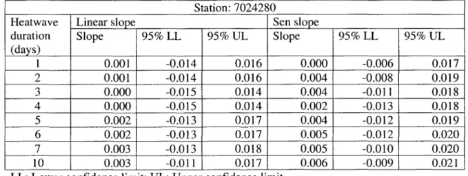
observed at four studied stations ... 28 Table A3. Linear regression and Sen's slope estimates for heatwaves observed at four studied

stations ... 29 Table A4. Lag-1 autocorrelation coefficients and their 95% confidence intervals ... 31

Table A5. The numbers of r_k values, that falls outside the confidence bands ... 31

Table A6a. p-values for F-tests of stability/equality of variance of a time series considering two sub-samples ... 32 Table A6b. p-values for F-tests of stability/equality of variance of a time series considering three

sub-samples ... 32 Table A7a. p-values for t-tests of stability/equality of mean of a time series considering two

sub-samples ... 33 Table A7b. p-values for t-tests of stability/equality of mean of a time series considering three

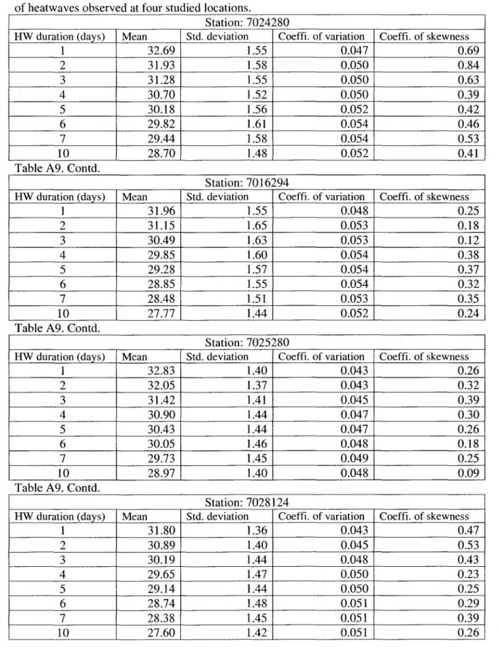
sub-samples ... 33 Table A8a. An ove rail summary of F-tests based on two and three sub-samples ... 34 Table A8b. An overall summary of t-tests based on two and three sub-samples ... 34 Table A9. Basic statistics (mean, standard deviation and coefficients of variation and skewness) of

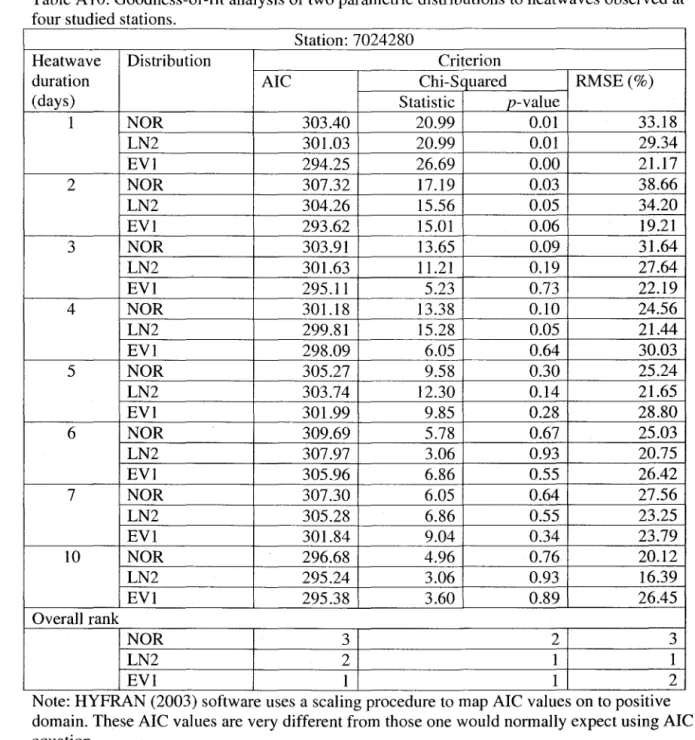
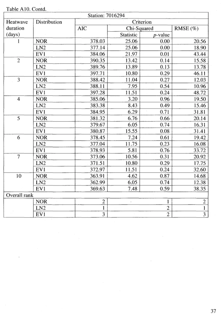
heatwaves observed at four studied locations ... 35 Table A 10. Goodness-of-fit analysis of two parametric distributions to heatwave data observed at

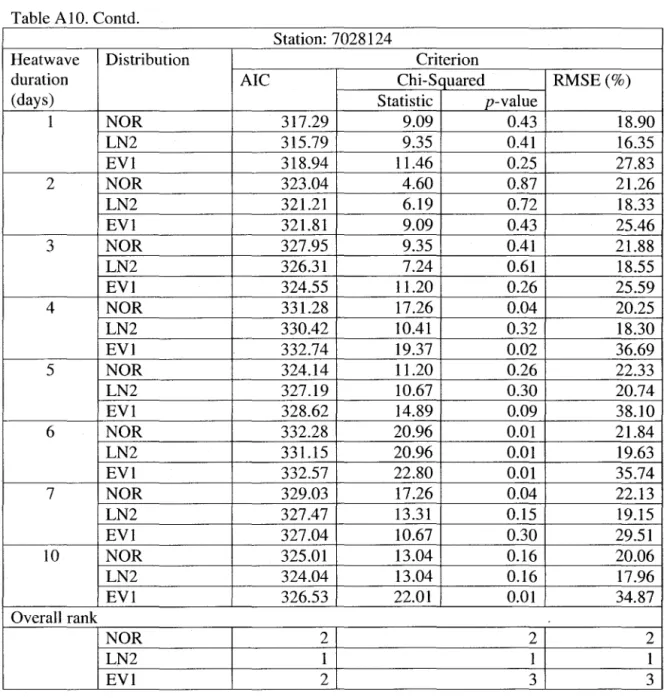
four studied stations ... 36 Table A 11. Goodness-of-fit analysis of three parametric distributions to heatwave data observed at

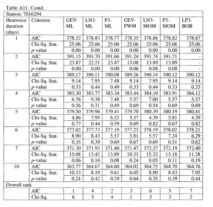
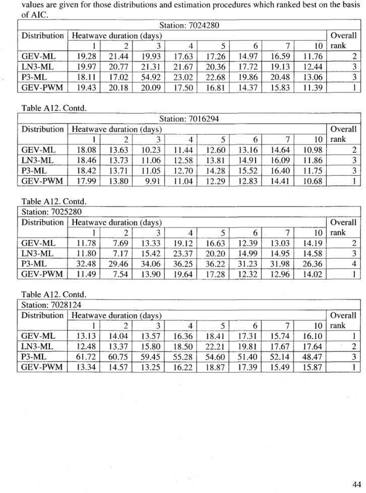
four studied locations ... 40 Table A 12. Goodness-of-fit analysis using root mean square error (RMSE) criterion. The RMSE

values are given for those distributions and estimation procedures which ranked best on the basis of Ale ... 44

(8)

Table A 13. Overall ranks after combining the results of two parametric and three parametric best fitting distributions ... 45

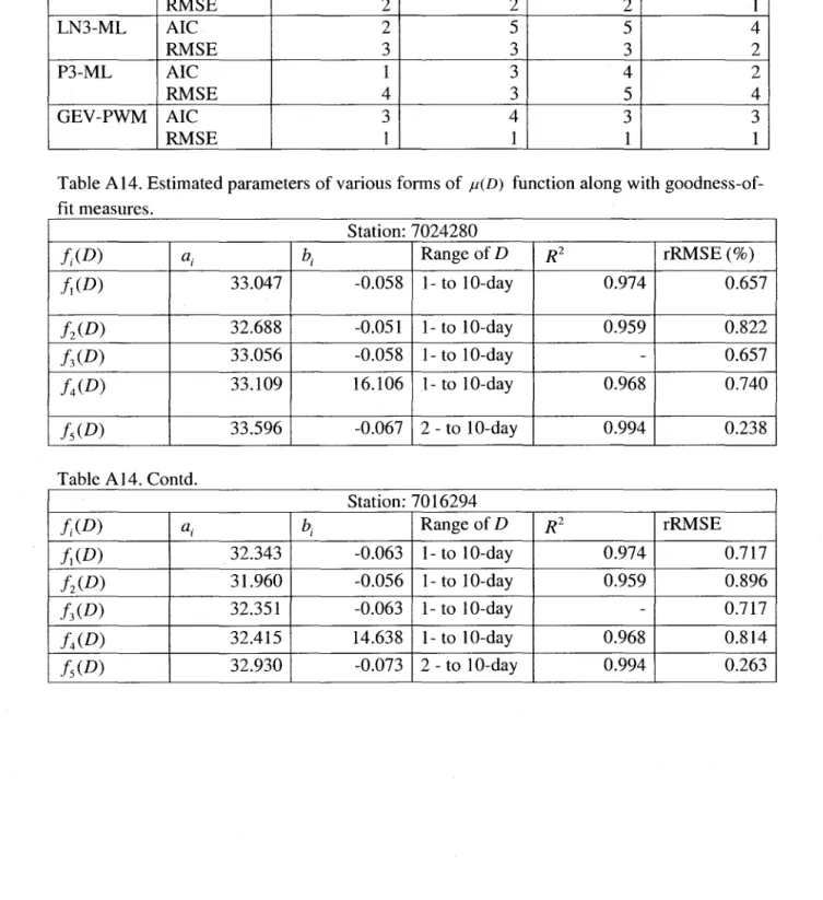
Table A 14. Estimated parameters of various forms of J'(D) function along with goodness-of-fit

measures ... 45

Table A 15. Results of Spearman's rank correlation and Mann-Kendall tests for starting dates of first

occurrences of heatwaves ... 47

Table A 16. Linear regression and Sen's slope estimates for starting dates first of occurrences of

(9)

LIST OF FIGURES

Figure No. and Caption ... Page No. Figure B1. A definition sketch for extraction of heatwaves of 1- and 2-day durations. Hl, is

the highest 1-day tempe rature and H 2, is the highest 2-day average temperature during

any year i ... 51

Figure B2. Time series plots of heatwaves (Ho series) of various durations along with linear trends observed at four studied stations ... 52

Figure B3. Correlograms of heatwaves of various durations. Solid, small dotted and large dotted lines represent 90%,95% and 99% confidence bands, respectively ... 56

Figure B4. Displays of basic statistics (mean, standard deviation, coefficients of variation and skewness) of heatwaves (Ho series) observed at four studied stations ... 60

Figure B5. Extreme value plots of heatwaves of 1-day to 10-day durations ... 62

Figure B6. L-moment ratio diagram of heatwaves (Ho series) for four studied stations. Small symbols (open circle, cross, open square and open triangle) represent observed values and corresponding large symbols represent group averages ... 64

Figure B7. At-site observed mean heatwaves and fitted f.l(D) functions. Fitting of f.l(D) functions consisted of mean heatwaves of 1 to 10 days duration ... 64

Figure B8. Site independent comparison of fitted f.l(D) functions. The closer the points are to the 11 D* line the better is the fitting ... 66

Figure B9. Fitting of GEV distribution to a selected set of observed heatwaves ... 67

Figure B10. Plots of standardized heatwaves along with fitted GEV distribution ... 67

Figure B11. Comparison of at-site growth curves ... 68

Figure B12. Comparison of estimated quantiles using models M1 to M5 with those of base model quantiles. Heatwave duration decreases along the "exact match" line. For each duration of heatwave, estimated quantiles appear as a group in vertical direction ... 68

Figure B13. Plots of base and modeled quantiles along with 95% upper and lower confidence intervals. CI-LL: Confidence intervallower limit, CI-UL: Confidence interval upper limit. ... 70

(10)

Figure B 14. Comparison of adequacy of models M 1 (extreme left bar) to M5 (extreme right bar) in preserving base model quanti les on the basis of relative root mean square error criterion ... 71 Figure B15. Dates of first occurrence and additional occurrences of heatwaves of same

magnitude in a year for heatwave durations of 1 to 10 days. Dot: first occurrence; Cross: second occurrence; Circle: third occurrence ... 72 Figure B16. Time series plots of dates (converted to Julian days) of first occurrence of

heatwave of indicated duration. Bracketed value is standard error of estimated slope .. 76 Figure B17. Quartile plots of dates of first occurrence of heat waves of 1-10 days

durations ... 80 Figure B18. Relationship between heatwave magnitude and date of first occurrence for

heatwave durations of 1-10 days. Relative frequencies are shown as stem plots (vertical lines) ... 81 Figure B19. Ten largest heatwaves and their corresponding dates of occurrence for

heatwave durations of 1-10 days. Vertical Lines (from left to right) represent end of May, June, July and August, respectively ... 85

(11)

SOMMAIRE EXÉCUTIF

Les extrêmes estivaux de température de l'air peuvent avoir un impact majeur sur la population humaine et même sur l'économie. Ces événements peuvent être caractérisés par leur amplitude

et leur durée. Les canicules sont non seulement définis par des températures maximales

journalières jugées extrêmes, mais aussi par une durée importante (i.e. plusieurs jours).

Le Groupe Impacts et Adaptation du consortium Ouranos a suggéré que les extrêmes de certaines variables climatiques jugées importantes pour le sud du Québec, telles que la température de

l'air, soient analysées statistiquement. Ces analyses permettent de mieux caractériser la

variabilité et les extrêmes de ces variables (ou des données dérivées) et permettent aussi de valider certaines méthodologies qui pourront ensuite être appliquées aux données provenant des simulations sous scénario de changements climatiques.

Les travaux de la présente étude ont donc pour objectif de valider une approche de type Intensité-durée-fréquence pour la caractérisation statistique des canicules dans le sud du Québec. Cette approche a été appliquée aux données de température de l'air maximum journalières provenant de quatre stations de la région, soit Montéral-McGill (7025280), Sherbrooke (7028124), Lennoxville (7024280) et Québec A (7016294).

La méthode utilisée consiste, en premier lieu, à calculer des séries de durée D Gours) à partir des séries de maximums journaliers. Pour ce faire, on calcule des moyennes mobiles sur une fenêtre de D jours pour toutes les stations. On extrait ensuite les maximums annuels de ces nouvelles séries de moyennes mobiles (D

=

1,2, 3,4, 5, 6, 7 et 10 jours). L'analyse fréquentielle est alors faite séparément sur chacune des 8 séries ainsi obtenues pour chaque station.

L'objectif de l'analyse fréquentielle consiste à trouver x_{T '}la variable ou quantile de retour T, de probabilité au non-dépassement p, où T

=

1/(1- p). On utilise des observations d'événements extrêmes passés afin d'estimer les probabilités futures d'occurrence. On doit, au préalable, vérifier l'hypothèse d'indépendance et de distribution identique (i.i.d.) des observations. On cherche ensuite à estimer les quantiles XT de période de retour T ou x_{p ,}la probabilité au non-dépassement tel que: x p == prob{ X ::;; x

T } == l-lIT. Pour ce faire, on sélectionne· une loi

statistique à partir de plusieurs modèles disponibles. La loi sélectionnée doit ensuite être ajustée aux séries de mesures, et l'estimation d'un quantile X_T par une estimation ponctuelle

x

_T est

alors donnée à partir de la loi ajustée.

Dans la présente étude, plusieurs lois ont été ajustées et ces ajustements ont été comparés. Par la suite, les quantiles estimés pour différentes périodes de retour T ont aussi été comparés pour différentes durées et un modèle général a été proposé.

Finalement, les dates d'occurrence des canicules ont aussi été analysées afin de confirmer ou infinner leur stationnarité (i.e. vérifier si la date d'occurrence de la canicule varie significativement au cours des années).

(12)

1.. L'amplitude des canicules est demeurée stationnaire au cours du siècle dernier, et ce, pour les quatre stations étudiées. Les valeurs moyennes des canicules de durée 10 jours ont varié entre 27,6 oc (Sherbrooke) et 29 oC (Montréal). Les canicules de durée 3 jours ont varié entre 30.19 oC (Sherbrooke) et 31.42 oC (Montréal).

2. L'évaluation de l'adéquation des distributions statistiques ajustées aux séries de canicules ont démontré que la loi log-normale est la meilleure loi à deux paramètres, tandis que la loi GEV semble être la loi à trois paramètres qui s'ajuste le mieux pour les échantillons provenant des quatre stations.

3. Les courbes Intensité-Durée-Fréquence obtenues ont un comportement mathématique similaire pour une station donnée et pour l'ensemble des séries étudiées. II devient donc possible de modéliser les quanti les de canicules de différentes durées à partir d'un facteur d'échelle et d'une courbe de croissance. Le facteur d'échelle établit la relation entre une valeur adimensionnelle de canicule et la période de retour T. La courbe de croissance est une distribution statistique adéquate pour tous les échantillons. La loi GEV (Generalized Extreme Value) a été utilisée comme courbe de croissance dans cette étude. Six différentes formulations mathématiques du facteur d'échelle ont été testées. Les erreurs relatives associées à chacune de ces formulations sont toutes inférieures à 1,5%. De plus, les courbes de croissance peuvent être estimées à partir de la courbe des quanti les de durée 1 jour, ce qui permet d'obtenir un modèle régional multi-durée simple à développer.

4. Une analyse des dates d'occurrence des canicules (date à laquelle commence une

canicule de durée D jours) a démontré que ces occurrences sont non-stationnaires dans

plusieurs cas. Ainsi, pour la station 7024280 (Lennox ville), une pente négative

significative existe pour les canicules de durée 1 à 4 jour, ce qui signifie que ces événements se produisent plus tôt dans l'année à la fin du siècle qu'au début de ce dernier. Cette conclusion s'applique aussi aux canicules (toutes durées confondues) de la station 7016294 (Québec A) et pour les événements de durée 1 à 3 jours à la station 7025280 (Montréal McGill). La station de Sherbrooke est aussi caractérisée par un avancement des dates d'occurrence de canicule de durée 1 à 3 jours au cours du siècle. Les canicules de durée supérieure à 5 jours ont plutôt tendance à se produire plus tard, comme en témoignent les pentes positives significatives des séries de date d'occurrence aux stations 7024280 (durée 6 et 10 jours), 7025280 (durée 4, 6 et 10 jours) et 7028124 (durée 6 à 10 jours).

(13)

1.0 INTRODUCTION

Extreme air temperature is known to have major effects on human populations, especially in

urban areas. It has been shown in many parts of the world that extreme maximum air

temperatures of long duration, the so-called heatwaves, can have adverse effects on public health (Rainham and Smoyer-Tomic, 2003; Duenas et al., 2002; Huth et al., 2000) and on the economy (Subak et al., 2000). Recently, Europe has experienced an intense heatwave that created vast health hazards and claimed thousands of lives (UK Guardian, 2003).

In Canada, a study performed in the nation's largest city (Toronto) investigated the link between

non-accidentaI human mortality and heat stress. A statistically significant relation was

established between the two variables measured for the period 1980-1996 (Rainham and Smoyer-Tomic, 2003). Although this study stated that the impact was minimal for the population of Toronto during this period, it is possible that the impact of heatwaves on urban population in Canada may bec orne a more serious public health problem in the future.

Bonsal et al. (2001) studied the characteristics of extreme temperatures over Canada. They found no significant trend over the course of the 20th century (1900-1998) for the higher percentiles of daily summer maxima. They concluded that the number of extreme hot days showed litde change during this period. However, mean annual temperature over Canada has increased by 0.9 OC between 1900 and 1998 (Zhang et al., 2000), and a recent climate change modelling study by Kharin and Zwiers (2000) has shown that daily maximum temperature extremes with a retum period of 20 years may increase by as much as 2.4 oC over the course of the next 50 years. In light of such findings and scenarios, it is of the utmost importance to develop statistical tools that may assist in providing a sound basis of comparison for future changes in extreme air temperature events such as summer heatwaves.

Frequency analysis is a widely used tool for describing the behaviour of hydro-meteorological variables, like flood peaks, low flows, flood volumes, drought duration, temperature and wind speed. To carry out frequency analysis, generally two different approaches are used to define the time series of the extreme variable of interest, i.e. annual maximum series and peaks-over-threshold series. Peaks-over-peaks-over-threshold series is also called partial duration series. In the annual maximum approach, only one value per year is used whereas in the peaks-over-threshold approach, there can be more than one value per year (i.e. aIl values above a certain threshold are included). In order to extract either annual maximum or peaks-over-threshold series from the observed data, instantaneous observations (e.g. flood peaks) or time-averaged observations (e.g. hourly rainfall intensity) or time-accumulated values (e.g. flood volumes, 24-hourly rainfall depth, degree-days) are used. Depending upon the type of analysis and application, other variables can also be defined and analysed. Haan (1977) and Cunnane (1989) document sorne hydro-meteorological variables which are often considered for frequency analysis. For methodological developments and application procedures of frequency analysis techniques in the areas of hydro-meteorology, the readers are referred to the reviews and comparison of techniques compiled by Cunnane (1989), GREHYS (1996), Madsen et al. (1997a, 1997b), Lang et al. (1999), Smakhtin (2001) and Katz et al. (2002).

(14)

Frequency analysis of rainfall of various durations has long been in use to develop rainfall intensity-duration-frequency (IDF) curves/relationships for sizing various hydraulic structures (Viessman et al., 1977). IDF curves can be developed for a particular site, for a geographical region or for a homogeneous region containing more than one site. Systematic methods for grouping a number of sites to form a homogeneous region have been developed by Hosking and Wallis (1997) in the context of regional flood frequency analysis. Sveinsson et al. (2002) and Ferro and Porto (1999) have developed regional IDF relationships for hydrologie al homogeneous regions following the approach of regional flood frequency analysis of Hosking and Wallis (1997). Inspired by the IDF analysis and regional flood frequency analysis, Javelle et al. (2000, 2002, 2003) have carried out flood-duration-frequency (QDF) analyses. In their studies, flood volumes were taken as accumulated flows over fixed durations and average flood flows were obtained by dividing the flood volume by the corresponding duration. Thus a 2-day flood was defined as the average of two consecutive days of maximum daily flows. Analogously, the present study is related to frequency analysis of daily maximum temperatures to characterize heatwaves. Merely performing a frequency analysis of daily maximum temperatures is not sufficient to interpret heatwaves, since these extreme events can only be full y described by associating duration with temperature magnitude. Therefore, in this work, a heatwave is defined as a run of consecutive days (say from 1-10 days) when the average daily maximum temperature is observed at the highest. This approach is referred to as heatwave-duration-frequency (HDF henceforth) analysis in the remainder of this report. The HDF concept is akin to the IDF and QDF approaches. Similarly to the QDF approach, a 2-day heatwave is defined as the largest average of two consecutive days of daily maximum temperature.

ln Southem Québec, maximum daily summer temperatures can exceed 30 oC during the summer months. In urban areas such as Montreal, such high temperatures may have adverse effects on public health, depending on their duration. The results of the HDF analysis would be useful to determine heatwaves of various retum periods and of various durations. It is hoped that this case study will complement the work done by Kharin and Zwiers (2000), who have used frequency analysis in their study of air temperature extremes but did not take into account the duration of events.

The dataset used in this work consists of relatively long series of daily maximum temperatures of four different locations in Southem Québec for the five months period from May to September. The data length ranges from 81 to 101 years. While July and August are the peak summer months, individual hot days or a group of two or three hot days have been observed as early as mid May and as late as during the second last week of September. Therefore, the analysis of daily maximum temperature series including the months of May to September guaranteed the inclusion of aIl peak values. The heatwave durations considered range from 1-10 days. At-site HDF analysis is performed using annual maximum series, index-flood method of Dalrymple (1960) and regional flood frequency approach developed by Hosking and Wallis (1997). In QDF analysis and in most of the regional frequency analyses, the index-statistic, which is used to standardize at-site data, is usually taken as the at-site mean. In this work, the index-heatwave for any duration is taken as the corresponding at-site mean value. Inspired from the regional flood frequency analysis and with sorne reasonably verifiable assumptions, the possibility of pooling standardized data across durations or adopting Hosking and Wallis (1997)' s regional frequency

(15)

analysis approach for at-site analysis, similarly as in Javelle et al. (2002,2003) for QDF analysis, is explored and studied in order to develop a parsimonious HDF approach.

This report is organized into various sections. In section 2, objectives of the research project are presented. A methodology is presented in section 3. The third section also contains a subsection on data screening to ascertain the quality of data used in this work. Detailed results of HDF analysis and pattern of occurrences of heatwaves are presented in section 4, followed by discussion and conclusions in section 5. Appendix A contains tables and Appendix B contains figures associated with this report. A summary of the non-parametric and parametric tests used for checking quality of data and Hosking and Wallis (1993)'s homogeneity test are presented in Appendix C.

2.0 PROJECT SPECIFIC OBJECTIVES

The main objectives of this project are summarized below:

• To perform exploratory data analysis of heatwaves to explore behaviours of basic statistics (i.e. mean, variance and coefficients of variation and skewness) in order to formulate appropriate modeling hypotheses.

• To set up a basis for performing frequency analysis of heatwaves in a parsimonious manner

o by modifying and utilizing the concepts and techniques developed for frequency analysis of other hydro-meteorological variables, and

o by selecting a suitable statistical model, on the basis of sorne model selection criteria, to de scribe the behaviour of D-day heatwave, where D is an integer number of days.

• To perform model validation.

• To study time-trends both in the magnitude and pattern of occurrences of heatwaves.

• To present and discuss results obtained and to identify future research directions.

3.0 METHODOLOGY

3.1

DATA EXTRACTION

As described earlier in the introduction section, a heatwave is a run of consecutive days with highest average daily maximum temperature (DMT). The time series of heatwave of duration D-day is denoted by HD • Thus for year i, H Di is the largest value of average maximum temperature

observed consistently for any D-day duration during May-September period (e.g. H3

i

=

30 oC if the observed daily maxima has been 30 oC during 3 consecutive days in year i). Similarly, J..lD

and Œ D are the mean and standard deviation of H_Dseries. For performing HDF analysis, DMT

data observed during May-September at four stations in Southern Québec, Canada is used. Station detail is given in Table Al.The length of data series ranges between 81 and 101 years. The peak summer period (i.e. July-August) is given more importance when deciding the Iength of record to be considered for analysis. For example, if for any year the DMT data for both July and August were missing then that year was not included in the analysis. As par definition of

(16)

heatwave, the temperature data for various durations needs to be computed from the DMT series. Temperature time series for various durations are extracted from DMT series using a moving

average with a window of width D-day (i.e. D

=

2-, 3-,4-,5-,6-, 7- and lO-day). The procedure

is explained in Figure BI. RD extreme values can thus be extracted from the original DMT series

to form new time series using either annual maximum or peaks-over-threshold approach. In this work, the annual maximum approach is used to extract RD series. Thus for every station, 8 samples (one for each duration) of RD series are obtained which constitute the basic set of data for the present analysis. Occasionally, reference has been made to RD series for D

=

15- and 30-day to verify sorne of the assumptions used in the analysis. However, these two RD series are not subjected to detailed analysis.

3.2

QUALITY OF

H

_DSERIES

For a successful frequency analysis, it is imperative to check data quality through graphical plots and statistical tests of significance. In graphical plots of sequential data, one can visually observe the presence of trends and jumps and the statistical tests help in explaining whether the trends and jumps, if any, are real or just because of sampling variability. There are two general approaches for testing quality of data: parametric and non-parametric. Parametric approaches make certain assumptions about the nature of data and non-parametric approaches do not make any assumptions about the underlying statistical distribution of the data. By making no assumptions about the distribution of the data, non-parametric tests are more widely applicable than parametric tests, which often require normality in the data. While more widely applicable, the trade off is that non-parametric tests are less powerful than parametric tests.

Two non-parametric tests, Spearman's rank correlation and Mann-Kendall tests are selected to verify the absence of trend and the independence of a time series (i.e. there is no correlation between the order in which the data have been collected and the increase or decrease in the magnitude of those data). Nevertheless, the independence of a time series depends on both the level of aggregation and separation in time of the data points. These tests are also recommended by WMO (WMO, 1966) for checking quality of hydro-meteorological data. To further strengthen the results of these two tests, Sen's (1968) non-parametric method is used to obtain an estimate of the magnitude of a monotonie trend. In addition to these non-parametric tests, ordinary linear regression slope and correlograms are used to verify absence of trend and independence of observations. Also, the t-test for stability of mean and the F-test for stability of variance are used to study stationarity of heatwave observations. A short description of aIl the above indicated tests is given in Appendix C.

Results of Spearman's rank correlation and Mann-Kendall tests are provided in Table A2. It is interesting to note that none of the RD series for ail the four stations exhibit any evidence of trend at 5% significance level. Results of Sen's slope are provided in Table A3. Again, the 95% confidence interval around the slope estimate does not support the presence of a monotonie trend in any of the RD series. Estimates of linear si ope, along with 95% confidence intervals are provided in Table A3. For obtaining linear slopes, linear regression was performed between values of RD series and time points. Plots of RD time series, along with linear slope estimates, are provided in Figure B2. AIso, the regression slope does not support the presence of a linear trend

(17)

at 5% significance level. Based on the results of all these tests, it can be conc1uded that HD data for all four stations are free of trends and jumps.

Computed values of lag-l autocorrelation coefficient, lj, and upper and lower limits of

confidence interval, at 5% significance level, are provided in Table A4. None of the lj values is significant at 5% significance level. The correlograms for Hl to HIO series are provided in Figure B3. In this figure, autocorrelations up to lag 20 along with 90%, 95% and 99% confidence intervals are plotted. For a quick inference, the numbers of r_k values, which fall outside the confidence intervals, are given in Table A5. None of the r_k values falls outside the 95% confidence interval for Hl to HIO series for station 7024280. For station 7025280, there is one r_k

value that faUs outside the 95% confidence band for Hl series. For station 7028124, there is one

r_k value that fans outside the 95% confidence band for each of Hl and H2 series. For station 7016294, there are two r_k values outside the 95% band for Hl series and one r_k value outside the 95% confidence band for each of the remaining series. Based on the 95% confidence bands, the only heatwave series that could be non-independent is Hl at station 7016294. In general, the above indicated significant r_k values are not extremely large because nearly an of them faU near the boundaries of confidence interval. Furthermore, the occurrences of significant r_k values are within the expected v ari ability , i.e. one out of 20 values is expected to faU outside the 95% confidence band. At a more conservative confidence interval (i.e. 90%), the occurrences of significant r_k values are within the expected variability for heatwave data of stations 7024280, 7025280 and 7028124. However, for heatwave data of station 7016294, there are two time series (i.e. H3 and HIO) which could be regarded as non-independent. In general, it seems that the quality of heatwave data of station 7016294 is relatively poor in comparison to other three stations.

The parametric tests used for testing stability/equality of variance and mean are the F-test and the t-test, respectively. These tests are based on the normality assumption. The requirement for normality is much less stringent for the t-test than for the F-test. One can apply the F-test for stability of variance and the t-test for stability of mean to data that belong to any frequency distribution, but the length of the sub-samples should be equal, or approximately so, if the distribution is skewed (Dahmen and Hall, 1990). Hence to apply these tests, the time series needs to be divided into two or three split, non-overlapping, sub-samples of approximately equal length. The heatwave time series are mildly skewed, so it is expected that the F-test will give an acceptable indication of stability of variance and the t-test for stability of mean. The t-test for stability of mean assumes that the variances of the two sub-samples are statisticaUy similar. The variances, can, however, differ only because of sampling variability. The test for stability of variance is usuaUy done first because instability of the variance implies that the time series is not stationary and is not suitable for a modeling exercise where one assumes stationarity of observations.

The results of F-test for stability of variance are provided in Table A6a for the case of two sub-samples and in Table A6b for the case of three sub-sub-samples. None of the heatwave series at an stations indicates instability of variance at 5% significance level (the same is true ev en at 10% significance level) when the time series were divided into two non-overlapping sub-samples of

(18)

approximately equal length. However, when using three sub-samples, the variance of Hl series, at station 7028124, is found instable at 5% significance level with one marginal case of Hl series at station 7016294. The results of t-test for stability of mean are provided in Table A 7a for the case of two sub-samples and in Table A 7b for the case of three sub-samples. None of the heatwave series at aIl stations indicates instability of mean (at 5% significance level) when the time series are divided into two non-overlapping sub-samples of approximately equal length. There are two significant cases at 10% significance level for station 7016294. When using three sub-samples, none of the time series showed any sign of instability of mean at 5% and 10% significance levels. Combined results of both F-test and t-test are provided in Tables A8a and A8b, respectively. Based on the results of F-test for stability of variance and the t-test for stability of mean, the Hl series at station 7028124 is probably non-stationary at 5% significance lev el. The number of non-stationary cases increases when using a more conservative significance level, e.g. 10%.

The results of statistical tests presented in this section indicate that there is one data series (Hl series at station 7016294) which could be non-independent at 5% significance level. However, the dependence is not very strong because firstly this non-independence vanishes at 1 % significance level and secondly the same series becomes independent at 10% significance level because the number of r_k values outside the 90% confidence interval is within allowed statistical variability. Furthermore, the values of the significant autocorrelation coefficients are within 6-22% of the 95% confidence intervals. Another data series (Hl series at station 7028124) is found non-stationary in the variance but stationary in the mean. However, the non-stationarity is dependent on the number of non-overlapping sub-samples the series is divided into in order to perform statistical tests for stability of variance. The non-stationarity vanishes wh en using two non-overlapping sub-samples. Thus, it is conjectured that inclusion of these two series into frequency analysis will have negligible effect on the overall results of the remaining large number of series. However, the results of frequency analysis of these two series should be interpreted with caution.

3.3

BASIC STATISTICS OF HDSERIES

Basic statistics (i.e. mean, standard deviation, and coefficients of variation and skewness) of aIl HD series are provided in Table A9 and plotted in Figure B4. It is useful to plot these statistics as a function of dependent variable to study their mutual variability and to formulate appropriate hypotheses. Plots of mean values in Figure B4 indicate that the mean J.1D is a decreasing function of duration and it decreases in a parabolic fashion. However, standard deviation CY D does not

depict a regular increasing/decreasing pattern as a function of duration. It fluctuates around a mean value randomly except for station 7016294 where it shows a regular decreasing trend after

D=2-day duration. Small values for the range of CY D for stations 7024280, 7025280 and 7028124

(i.e. 0.12, 0.09 and 0.12, respectively) and increase in coefficient of variation as duration

increases (Figure B4) suggest that the assumption of duration-independent value of CY_D would be

appropriate for these stations. For station 7016294, where a decreasing trend after D=2-day duration is realized, the assumption of duration-independent value of CY D is appropriate for a

subset of durations. However, overall small range of CY D (i.e. 0.20) for this station also suggests

(19)

Both Table A9 and Figure B4 indicate that BD series are just moderateIy skewed, i.e. coefficient of skewness ranges between 0.39 and 0.84 for station 7024280, between 0.12 and 0.37 for station 7016294, between 0.09 and 0.39 for station 7025280 and between 0.23 and 0.53 for station 7028124. One could expect that BIO series should present minimum value of coefficient of skewness because each value in this series is an average of 10 consecutive values. The minimum value of skewness is observed for B4 series at station 7024280 and 7028124, for B3 series at station 7025280, and for BIO series at station 7025280. A regular decrease in skewness as duration increases can probably be hypothesized in the case of station 7028124. However, small range of coefficient of skewness indicates that it could be possible to assume a duration-independent value of skewness for aIl heatwave series at each station. The above presented behaviours of basic statistics, particularly the dominance of scale, are exploited in the domain of L-moments (Hosking, 1990) to formulate appropriate hypotheses in order to deveIop a parsimonious at-site HDF approach.

3.4

SELECTION OF A STATISTICAL DISTRIBUTION FOR

H

_DSERIES

Extreme value plots of heatwaves are provided in Figure B5 for the four studied stations. Extreme values are plotted against Extreme Value type 1 (EVl) reduced variate using Gringorton plotting position formula: p

=

Ci -

0.44) /(n

+

0.12), where i is the rank in ascending order and n is the number of observations. Such plots help one to decide about the suitability of the EVl (or Gumbel) distribution for modelling purposes. A straight line plot would suggest that the EV 1 distribution is a strong candidate model. The plots of Figure B5 show moderate downward curvature except for station 7024280, for which plots tend to follow straight lines. Another obvious observation is that the plots of extreme values of various durations demonstrate a parallei behaviour, except for few observations at both tails. This behaviour suggests that scale is a dominant factor and if the effect of sc ale is removed then aIl the plots could overlap each other. The effect of scale is studied in a subsequent section.

In order to model values of BD series, sorne of the 2-parameter and 3-parameter statistical distributions are analyzed and no attempt has been made to perform an exhaustive analysis in this respect. The 2-parameter distributions include the Normal (NOR), Lognormal (LN2), and Extreme Value Type l (EVl). The 3-parameter distributions include the Generalized Extreme Value (GEV), Lognormal (LN3), Pearson Type III (P3) and Log Pearson Type III (LP3). For 2-parameter distributions, only maximum likelihood (ML) estimators are used. For the LN3 and P3, both ML and ordinary moment (MOM) estimators are used. For the GEV, both ML and probab il it y weighted moments (PWM) estimators are used. LP3 distribution is fitted using the procedure described by Bobée (1975). AlI of the parameter estimations are performed using HYFRAN (2003) software. The choice of a best fitting model is performed on the basis of three modeI selection criteria, i.e. Akaike Information Criterion (AIC), Chi-squared test statistic and Root Mean Square Error (RMSE).

The Chi-squared goodness-of-fit statistic is weIl documented in most of the statistical books (e.g. Snedecor and Cochran, 1989), and is not repeated here. This test is very sensitive to the number of classes in which the empirical distribution is divided into. It is possible that if the test statistic is significant with nI class intervals then it may not be significant with n2 (where n2 being greater

(20)

than or less than nI) class intervals. For ca1culating class intervals, HYFRAN (2003) software is used and no attempt has been made to analyze the effect of class intervals because the chi-squared test statistic is not used to perform a test of significance rather its magnitude is used for ranking purposes to distinguish a statistical mode! that gives the smalIest value of the test statistic in a manner similar to AIC and RMSE criteria. Thus among a group of competing models, the one that gives minimum value of the Chi-squared test statistic is the best fitting model on the basis of Chi-squared test statistic criterion and the one that gives the minimum value of the AIC is the best fitting model on the basis of Ale. Similar argument is applicable for RMSE criterion.

Various forms of AIC have been used in literature. The form of AIC varies with respect to how the test statistic is penalized for the estimated parameters and record length. The form of AIC used in this work is given below:

AIC

=

-2 ln (ML) + 2m (3.1)

where ML denotes the maximum likelihood and m denotes the number of fitted parameters. The

AIC is employed to select the best fitting model. The best fitting model is the one with the smalIest value of AIC. AIthough the AIC goodness-of-fit criterion is constrained to maximum likelihood estimation, it has been used regardless of the estimation method (Strupczewski et al., 2001; Mutua, 1994).

The use of RMSE for model selection is demonstrated by Cunnane (1989) and a variant of it by Yu et al. (1993). This criterion is evaluated as folIows:

(3.2)

where Xi and Xi are respective!y the observed and estimated quantiles corresponding to ith plotting position and n is the record length. In order to estimate the value of this criterion, one needs to select an appropriate plotting position formula. A number of plotting position formulae have been proposed in the literature for various distributions. Cunnane (1989) analyzed that the choice of a best fitting distribution using RMSE criterion is independent of the plotting position formula and method of parameter estimation (i.e. maximum likelihood and moments). Cunnane (1978) proposed a single distribution free formula as a reasonable compromise for mildly skewed data and same has been used to compute RMSE in the present work. The current dataset is mildly skewed and hence, the choice of Cunnane plotting position formula seems reasonable. A model that gives smalIest value of RMSE is considered the best fitting model among a group of competing models.

For the 2-parameter distributions, the values of AIC, Chi-squared and RMSE are given in Table AlO. AlI three criteria suggest that LN2 is the overall best fitting distribution. However, EVI is another equally likely choice for station 7024280. The choice of best fitting distribution is made as follows: for each record, each distribution is assigned a rank between 1 and 3, rank 1 for the best fitting distribution (e.g. the distribution having lowest value of Chi-squared test statistic).

(21)

For each distribution, the ranks are summed over aIl 8-durations and these totals of ranks are used to choose a best fitting distribution. Table AlI presents the values of AIC and Chi-squared criteria for 3-parameter distributions. As commented earlier, the value of Chi-squared test statistic is very sensitive to the number of class intervals. Renee, the Chi-squared test statistic criterion is not used to distinguish best fitting 3-parameter distributions. Based on AIC criterion, first four best fitting distributions are GEV-ML, LN3-ML, P3-ML and GEV-PWM. The RMSE for these four best fitting distributions are given in Table A12. According to RMSE, the order of best fitting distribution for stations 7024280 and 7016294 is GEV-PWM, GEV-ML, LN3-ML, and P3-ML, with the last two being at the same rank. For station 7025280, the order is PWM, ML, LN3-ML, and P3-ML. For station 7028124, the order is PWM, GEV-ML, LN3-GEV-ML, and P3-GEV-ML, with the first two of the same rank. Combined results of AIC and RMSE for 2-parameter best fitting distribution (i.e. LN2) and 3-parameter distributions are given in Table A13. Based on AIC, overall best fitting distribution is the GEV -ML and based on RMSE the best fitting distribution is the GEV-PWM.

The L-moment ratio diagram for RD series is provided in Figure B6. The definitions and methods

of computing L-moments, which are linear combination of order statistics, of various commonly used distributions are given in Hosking (1990). The moment ratio diagram represents the L-kurtosis of a sample as a function of its L-skewness. In this diagram, two parameter distributions are defined as points and three parameter distributions are defined as curves. The L-moment ratio diagram given in Figure B6 suggest that the points of sorne of the RD series are located more close to Generalized Pareto distribution (GPD) curve as compared to curves of LN3, P3 and GEV distributions. However, none of those series which faIl near GPD curve could be fitted by GPD when its parameters were estimated by method of moments and probability weighted moments because the upper bound of the distribution was always smaller than the maximum value of the observed sample. The points of RD series of 7016294 and 7025280 sUITound LN3, P3 and GEV curves indicating that any one of them could be a suitable choice for these two stations. However, this behavior is less obvious for the remaining two stations particularly in the case of 7024280. The L-moment ratio diagram is provided here for the sake of completeness rather being used as a model selection criterion.

Based on the above presented results and discussion, the GEV-PWM distribution is selected for modeling RD series for aIl four stations. One obvious conclusion is that the Normal distribution that has been used by Wettstein and Mearns (2002) to model daily maximum temperature series cannot be selected as the best fitting distribution on the basis of AIC and RMSE criteria for the CUITent dataset.

3.5

HEATWAVE MAGNITUDE-DuRATION-FREQUENCY (HDF) ApPROACH

The RDF analysis presented here is restricted to D=l-, 2-, ... , 7-, and lO-day durations. It is possible to extend the analysis beyond 10-day duration but in that case the usefulness of

heatwave may become meaningless. The aim of the HDF modeling is to de scribe the RD

distributions in a parsimonious manner by adopting the methodology of regional index-flood frequency analysis. Similar approach has been adopted by Javelle et al. (2002, 2003) for QDF analysis. It is assumed that for any site the T-year heatwave, RD (T), can be expressed as the product of two terms. These two terms are the scale factor, f.l D' and the growth factor, g(T). The

(22)

scale factor is called the index-heatwave and the growth factor describes the relationship between dimensionless heatwave and the recurrence interval, T. The index heatwave is duration dependent while the growth curve is assumed to be valid for the entire group of HD distributions. This can be eXplained by the following relationship:

H(D,T)

=

f.1(D)g(T) (3.3)

where H(D,T) is the modeled value of H D (T) and f.1(D) is the modeled value of f.1D and g(T) is a dimensionless parent fitted distribution, with a mean of 1. This implies that aIl H D (T)

distributions approach the same distribution wh en standardized by the respective mean value and this assumption is in parallel to behaviors of basic statistics presented in section 3.3 and further verified in section 4.2. Based on the analysis presented in the above section, g(T) is taken to be GEV distribution with probability distribution function given by

fy(y;u,a,k)

=

(lI a)[l-k(y-u)1

ar

l+l/k xexp{-[I-k(y -u)1 a]J/k} (3.4) where, - 00 < u, a > 0, and k are the location, scale and shape parameters respectively. The

range of y is such that 1-k(y - u) 1 a >

o.

The return level which is exceeded once every T years on average, is given by

Y(T)

=

u

+

(a 1 k)[l- (-ln(l-I/T)/]. (3.5)

The parameters of the GEV distribution can be estimated either by pooling standardized observations across durations and thereby estimating parameters from the pooled sample or from standardized PWMs averaged across durations. The later approach, which is weIl documented by Hosking and Wallis (1997) for regional frequency analysis, is adopted here. The averaged standardized probability weighted moments are defined below:

(3.6)

where ber) is the rth PWM of g(T), bD(r) the rth PWM of H D distribution, bD(1) is the first PWM of HD distribution which is equivalent to f.1 D and ND is the number of durations. The PWM parameter estimation for the GEV distribution is given in Hosking et al. (1985).

The scale factor f.1D can be modeled as a function of D similarly as in Javelle et al. (2002, 2003) for QDF analysis and as in Ferro and Porto (1999) for regional IDF analysis. The general form of this relationship is given by

(23)

Six different fonns of f(D) are assumed and analyzed. These different fonns of f(D) are given below (where a and b are parameters of the function):

(3.8) (3.9) (3.10) F (D) _ a4 )4 -1+ln(D)/b 4 (3.11)

J

f5 (1)

=

,ul lf5 (D)

=

a_5Db5 for D

=

1

for D

=

2-,3-, ... , 7 -, and 10 - day (3.12)

(3.13)

The fonns J;(D), f2(D), f~(D) and f6(D) are fitted to ,uD values using a least squares approach by linearizing the functions through log-transfonnation, the fonn f4 (D) is fitted using a least squares approach by linearizing the function through inverse-transfonnation and the fonn

f3 (D) is fitted following the minimization approach introduced by Javelle et al. (2002). The

rational behind studying six functional fonns of f(D) is explained below.

The functional fonn

fI

(D) has been used by Ferro and Porto (1999) and Porras and Porras (2001) for IDF analysis and is included here to investigate if same functional fonn could also be used for HDF analysis. However both of these studies also noticed the duration dependent functional fonn of f(D) relation, i.e. multiple functional fonns govem the ,u(D)

=

f(D)

relationship. This possibility of multiple relations is also investigated in the case of HDF analysis by hypothesizing f5 (D) functional fonn for modeling ,u2 to ,u1O and ,ul independently. Thus the functional fonn

f

₅(D) has total of three parameters as opposed to aIl other fonns. The functional fonn f2 (D) is designed to study if the ,uD values for D=2- to lü-day can be scaled from,ul . The parameter b2 of this fonn can be estimated through least squares approach first by dividing each ,uD value by ,ul' perfonning log-transfonnation and setting constant to zero. The functional fonn f3 (D) is exactly same as

fI

(D) but differs with respect to the fitting procedure. The

fI

(D) functional fonn is fitted through least squares method and f3 (D) is fitted using the method of Javelle et al. (2002), i.e. the parameter b3 is estimated by minimizing the following error criterion:

(24)

(3.14)

where n is the number of values within each sample of HD • "X(j) is the mean ordered observed duration scaled value given by

(3.15)

where x_D; (j) is the duration scaled value obtained by dividing the H D; (j) value by Db,. The

parameter G 3 is taken as the average of "X(j) series. The above equation implies that "X(j) is computed by taking average of duration scaled ordered values across durations. This implies that sample size has to be same for each HD series. If the sample size is different for each HD series (which could result in case of peaks-over-threshold approach), then this approach cannot be applied and recourse has to be made to an alternate method given in Javelle et al. (2003) or to sorne other appropriately designed methods. The above described parameter estimation procedure is included here to find the effect of parameter estimation procedure on the estimated parameters. It is necessary to mention here that Javelle et al. (2002) used "X(j) series to estimate quantiles of the averaged series for scaling purposes to estimate quantiles corresponding to various durations. Their approach for estimating H (D, T) quantiles is retained here for comparison purposes. The functional form f4 (D) is designed as an alternative to f6 (D), which has been used by Javelle et al. (2002, 2003) for QDF analysis. The functional form f6 (D) is included here for comparison purposes and to investigate if same could be used for HDF analysis. It is important to mention here that no physical meanings are associated with parameters of any of the functional form f(D) and focus has been on how weIl the f.1D values

can be modeled.

Site independent comparison of f(D) functions can also be performed by defining the following

quantities:

f* (D) = f(D)/ Gand (3.16)

D* =I/Db and D* =l/(l+lnD/b). (3.17)

The quantile estimates of heatwave of any desired return period T and any desired duration D depend upon the choice of scaling function (i.e. fI (D) to f6 (D») and upon the type of quantiles being scaled, i.e. dimensionless quantiles given by g(T) or H(l,T) quantiles or quantiles of averaged series "X(j). For the sake of presentation convenience, these combinations are given acronyms as eXplained below:

(25)

Model 1 (Ml) - The H (D, T) quantiles for this case are estimated using

fI

(D) functional form of f.l(D) and g(T) dimensionless quantiles, i.e.

(3.18)

Model 2 (M2) - The H(D,T) quantiles for this case are scaled from H(1,T) quantiles using

f2 (D) functional form of f.l(D). H (1, T) quantiles are estimated by fitting GEV distribution to HI series using PWMs.

Model 3 (M3) - The H (D, T) quantiles for this case are estimated by scaling the quantiles obtained by fitting GEV distribution to x(j) series with f3 (D) functional form of f.l(D).

Model4 (M4) - The H(D,T) quantiles for this case are estimated similarly as in the case of Ml but using f4 (D) functional form of f.l(D).

ModelS (MS) - The H(D,T) quantiles for this case are estimated similarly as in the case of Ml but using f5 (D) functional form of f.l(D).

Model6 (M6) - The H(D,T) quantiles for this case are estimated similarly as in the case of Ml but using f6 (D) functional form of f.l(D).

Having obtained H(D,T) quantiles for a set of durations and return periods, heatwave

magnitude-duration-frequency relationships can be established.

3.6

PATTERN OF OCCURRENCES OF HEATWAVES

The pattern of occurrences of heatwaves (i.e. values of HD series) is studied by extracting the time series of starting date (denoted by SDD) of heatwave and converting it into Julian days. For any year i, the value of SD_I, is the day of the year when the highest DMT occurred and the value

of SD3, is the day of the year wh en highest 3-day average DMT started occurring.

The time trends in the pattern of occurrences are analysed using Spearman's rank correlation and Mann-Kendall non-parametric tests. The results of these tests are further supported using Sen' slope and linear regression slope estimates.

4.0 RESULTS

The HDF approach presented above is applied to DMT series observed at 4 stations in Quebec and results for these stations are presented with respect to validation of HDF approach, i.e. fitting

(26)

magnitude-duration-relationships and their adequacy in preserving base model quantiles. Finally, the pattern of occurrences of heatwaves is presented.

4.1

FUNCTIONAL FORMS OF f-l(D) FUNCTION

The estimated parameters of aIl functional forms of f-l(D) are given in Table A14. The R2

values are also provided in this table wh en the parameters are estimated through least squares approach. The Relative Root Mean Square Error (rRMSE) values are also provided as an alternate measure for goodness-of-fit of the functional form. It is interesting to note that R2

values are quite high (> 0.95) for aIl functional forms indicating that any one functional form can be assumed to model f-l(D)

=

f(D) relationship. To visuaIly compare this relationship, the plots of observed and modeled values of f-lD are provided in Figure B7. In this figure, the functional forms are also compared with respect to extrapolation, i.e. how weIl they perform beyond the range used for estimating their parameters. The relationships are extrapolated up to D=30 days. It is obvious from Figure B7 that the functional form f6 (D) does not foIlow the trend of f-lD curve. Hence, this form is not an appropriate choice to model f-l(D)

=

f(D) relationship for heatwaves and the results of analysis using this form are not included in the remainder of this work. The estimated parameters of fi (D) and f3 (D) are almost similar and hence they perform similarly.

There is almost negligible effect of estimation method on the estimated parameters. The

f

₂(D)

functional form preserves f-ll but generally underestimates f-l2 to f-l5 values and overestimates in the extrapolated region. The f4 (D) functional form performs almost similarly as

fi

(D) and

f3 (D). The functional form f5 (D) preserves f-ll' performs very weIl both in the parameter estimation region and in the extrapolated region. Although f-l15 and f-l30 are not used for fitting

f5 (D) function, it provides reasonably good estimates of those values. The weIl behaved nature of f5 (D) can be partly explained as foIlows. The HD series can be divided into two domains i.e.

one without any averaging (i.e. Hl series) and another with averaging (i.e. H2 to H30 series). It seems that these two domains need to be modeled independently - this observation supports the findings of Ferro and Porto (1999) and Porras and Porras (2001) for noticing more than one functional form for sorne datasets.

Site independent comparison of f(D) functions is provided in Figure B8 where f* (D) and D*

values are plotted. The closer the plotted points are to the l/D* line the better are the estimated values. The extrapolated region for the f5 (D) case is also shown in this figure. The lower part of the curve presents the extrapolated region where the plotted points are very close to l/D* line. From the results presented above, it is obvious that the f5 (D) functional form performs very well. For aIl the stations, the relative error between f-lD and corresponding modeled value for

1;

(D) and f3 (D) varies between -1.0% and 1.2%, for f₂(D) between -1.4% and 1.2%, for

f

4(D) between -1.1% and 1.4% and for

f

5(D) between -0.4% and 0.5%. The rRMSE given in

(27)

appropriate for modeling Il(D)

=

f(D) relationship for the current dataset while other forms,

fI

(D), f3 (D) and f4 (D), also provide reasonable estimates of IlD. AlI functional forms of Il(D) are considered for the remaining analysis presented here.

4.2

DEVELOPMENT OF AT-SITE GROWTH CURVE

The fitting of GEV distribution to a selected set of HD series is provided in Figure B9. It is obvious that the GEV distribution provides a good fit to observed data at aIl four stations. The quantitative measures of goodness-of-fit have already been presented and discussed in a previous section on model selection. The quantiles H D (T) estimated by fitting the GEV distribution to

each individual HD series are referred to as base model quantiles for comparison purposes while assessing the validity of HDF modelling approach.

It is hypothesized in the previous section that if the effect of scale is removed by standardizing HD extreme values then all plots would overlap each other. This is demonstrated in Figure BIO

where standardized plots along with fitted GEV distribution are provided. AlI standardized empirical distributions overlap each other and the GEV distribution provides a good fit to standardized data. Thus it is safe to assume that various H D (T) distributions are linked through

a scale factor. The validity of this assumption is investigated using Hosking and Wallis (1993)' s homogeneity test, which was specifically devised for defining homogeneous group of stations, by extending its definition from a group of stations to a group of hydro-meteorological series

(HD series in the present context) at a single site. A summary of this test is provided in Appendix C. To apply this test for at-site HD series, vector Bootstrap technique (Efron and Tibshirani, 1994) was used to evaluate W_k statistics. It was found that W_k statistics were much less than 1 at all four studied stations. This indicates that at-site standardized HD series can be pooled together to form a homogeneous group and, hence, to derive a common at-site growth curve. The suitability of a common at-site growth curve is again verified by comparing H D (T) and

H(D,T) quantiles in section 4.3.

The GEV produced g(T) growth curves for aIl four stations are plotted together in Figure Bll and they differ from each other in extreme upper and Iower tails onIy. Although there are small differences from one growth curve to the other, it is not possible to assume a single growth curve for these four stations without providing any physical justification with respect to weather producing mechanisms that prevail over these stations during summer season. This aspect is beyond the scope of present study. It is worth mentioning that almost negligible differences were

found between growth curve, g(1), parameters and quantiles using average standardized PWMs

and PWMs of standardized pooled sample. Thus either approach is equally applicable. This observation indicates that non-parametric density estimation methods can also be used to obtain

g(T) growth curve using standardized pooled sample.

4.3

HEATWAVE MAGNITUDE-DuRATION-FREQUENCY RELATIONS

Estimated quantiles for models MI to M5 are plotted in Figure B 12 against base model quantiles, which are estimated by fitting the GEV distribution to each HD series. The line of perfect fit help

(28)

quickly determine the under- or over-estimation. Overall best estimates are provided by mode!

M5 while mode! Ml, M3 and M4 perform similarly but always over-estimate H (1, T) quantiles.

Model M2 provides exact estimates of H (1, T) quantiles, relatively better estimates of H (1 0, T) and poor estimates of quantiles of heatwave of other in-between durations (i.e. H (2, T) to

H (7, T» and difference between base and estimated quantiles increases as retum period increases. The significance of over- or under-estimation of base quantiles can be assessed by plotting aIl estimated quantiles within 90% or 95% or 99% confidence bands. 95% confidence interval is se!ected here. AlI estimated and base quantiles along with 95% confidence band for 2 and 50 year retum periods are plotted in Figure B 13. The 95 % confidence intervals are estimated using vector Bootstrap technique (Efron and Tibshirani, 1994). It is hoped that the Bootstrap technique would provide reasonable estimates because of re!atively large sample sizes used in this work. In order to determine the number of replicates required to obtain stable estimates of confidence intervals, estimates were obtained for 200, 500, 1000, 2000, 5000, 10000 replicates and assessed against those obtained from 20000 replicates. It was found that 10000 replicates are sufficient to obtain stable estimates of confidence intervals. Rence, the values located at 2.5% and 97.5% position were taken as lower and upper 95% confidence intervals. Figure B 13 indicates that the quantiles estimated with model M5 generaIly lie right inside the 95% confidence band for aIl durations at aIl sites. The H (1, T) quantiles estimated with models Ml, M3 and M4 lie at the boundary of upper 95% confidence interval and those for other durations inside the confidence band. The H (2, T) to H (6, T) quantiles estimated with model M2 lie at or near the lower boundary of 95% confidence interval. It is expected that if the confidence interval is expanded to 99% then they might fall inside the confidence interval.

The adequacy of MI to M5 models in preserving the base model quantiles is also assessed on the basis of rRMSE criterion. The plots of rRMSE for various models are provided in Figure B 14. The rRMSE varies between 0.77% (7025280) and 0.88% (7016295) for Ml, between 1.1 % (7025280) and 1.39% (7028124) for M2, between 0.78% (7025280) and 0.88% (7016294) for M3, between 0.85% (7025280) and 0.98% (7016294) for M4 and between 0.47% (7024280) and 0.59% (7028124) for MS. The rRMSE is generaIly smaIl for small retum periods and large for large retum periods. The rRMSE is the lowest for MS for aIl the four stations and almost indifferent for Ml and M3. Although the rRMSE for M2 is highest among aIl models for aIl stations, the overall performance can be considered adequate (rRMSE<2%). This method is of particular interest because of the manner in which various quantiles are scaled. The useful feature of this approach is that it would permit to derive quantiles of heatwave of higher durations from quantiles of heatwave of I-day duration only.

4.4

PATTERN OF OCCURRENCES OF HEATWAVES

Time series of starting dates of first occurrence of heatwave, SDD, were extracted from the

historical observations and are plotted in Figure B 15. It was observed that in sorne years the heatwave of same magnitude had occurred more than once. Therefore, the starting dates of additional occurrences were also extracted and plotted in Figure B15. It can be seen from this figure that in sorne years, at most three occurrences of the same heatwave had occurred and this observation is uniform across ail four stations. In general, the frequency of second occurrence either decreases or stays almost constant as the duration of heatwave increases. Third occurrence

Frequency analysis of daily maximum temperature in southern Québec with a view to interpret heatwaves = Analyse frequentielle des températures maximum journalières du sud du Québec pour des fins d'interprétation des canicules.

FREQUENCY ANALYSIS OFDAILY

MAXIMUM TEMPERATURE IN

SOUTHERN QUÉBEC WITH A VIEW

TO INTERPRET HEATW A VES

c-~

C>UR4,..,C>S

FREQUENCY ANAL YSIS OF DAIL Y MAXIMUM

TEMPERATURE IN SOUTHERN QUÉBEC WITH A

VIEW TO INTERPRET HEATW A VES

ANALYSE FREQUENTIELLE DES TEMPÉRATURES

MAXIMUM JOURNALIÈRES DU SUD DU QUÉBEC POUR

DES FINS D'INTERPRÉTATION DES CANICULES

M.

Naveed Khaliq

André St-hilaire

Taha B.M.]. Ouarda

Bernard Bobée

TABLE OF CONTENTS

LIST OF TABLES

LIST OF FIGURES

SOMMAIRE EXÉCUTIF

=

=

x

1.0

INTRODUCTION

2.0 PROJECT SPECIFIC OBJECTIVES

3.0 METHODOLOGY

3.1

=

=

=

3.2

H

3.3

3.4

H

=

Ci -

+

=

3.5

=

=

ar

o.

=

+

J

=

=

=

=

fI

=

f

fI

fI

fI

3.6

4.0 RESULTS

4.1

=

=

f

fi

1;

f

f

=

fI

4.2

4.3

4.4