arXiv:1210.2329v2 [astro-ph.EP] 16 Jan 2013
January 17, 2013
WASP-54b, WASP-56b and WASP-57b:
Three new sub-Jupiter mass planets from SuperWASP
⋆
F. Faedi
∗1,2, D. Pollacco
∗1,2, S. C. C. Barros
3, D. Brown
4, A. Collier Cameron
4, A.P. Doyle
5, R. Enoch
4, M. Gillon
6, Y.
G ´omez Maqueo Chew
∗1,2,7, G. H´ebrard
8,9, M. Lendl
10, C. Liebig
4, B. Smalley
5, A. H. M. J. Triaud
10, R. G. West
11, P.
J. Wheatley
1, K. A. Alsubai
12, D. R. Anderson
5, D. Armstrong
∗1,2, J. Bento
1, J. Bochinski
13, F. Bouchy
8,9, R.
Busuttil
13, L. Fossati
14, A. Fumel
6, C. A. Haswell
13, C. Hellier
5, S. Holmes
13, E. Jehin
6, U. Kolb
13, J.
McCormac
∗15,2,1, G. R. M. Miller
4, C. Moutou
3, A. J. Norton
13, N. Parley
4, D. Queloz
10, A. Santerne
3, I. Skillen
15, A.
M. S. Smith
5, S. Udry
10, and C. Watson
21 Department of Physics, University of Warwick, Coventry CV4 7AL, UK
e-mail: [email protected]
∗ part of the work was carried out while at Queen’s University Belfast
2 Astrophysics Research Centre, School of Mathematics and Physics, Queen’s University Belfast, University Road, Belfast BT7
1NN.
3 Aix Marseille Universit, CNRS, LAM (Laboratoire d’Astrophysique de Marseille) UMR 7326, 13388, Marseille, France 4 School of Physics and Astronomy, University of St. Andrews, St. Andrews, Fife KY16 9SS, UK
5 Astrophysics Group, Keele University, Staffordshire, ST5 5BG, UK 6 Universit´e de Li`ege, All´ee du 6 aoˆut 17, Sart Tilman, Li`ege 1, Belgium
7 Physics and Astronomy Department, Vanderbilt University, Nashville, Tennessee, USA 8 Institut d’Astrophysique de Paris, UMR7095 CNRS, Universit´e Pierre & Marie Curie, France 9 Observatoire de Haute-Provence, CNRS/OAMP, 04870 St Michel l’Observatoire, France
10 Observatoire astronomique de l’Universit´e de Gen`eve, 51 ch. des Maillettes, 1290 Sauverny, Switzerland 11 Department of Physics and Astronomy, University of Leicester, Leicester, LE1 7RH
12 Qatar Foundation, P.O.BOX 5825, Doha, Qatar
13 Department of Physical Sciences, The Open University, Milton Keynes, MK7 6AA, UK
14 Argelander-Institut f¨ur Astronomie der Universit¨at Bonn, Auf dem Hgel 71, 53121, Bonn, Germany 15 Isaac Newton Group of Telescopes, Apartado de Correos 321, E-38700 Santa Cruz de Palma, Spain
Received; accepted
ABSTRACT
We present three newly discovered sub-Jupiter mass planets from the SuperWASP survey: WASP-54b is a heavily bloated planet of mass 0.636+0.025
−0.024MJand radius 1.653 +0.090
−0.083RJ. It orbits a F9 star, evolving off the main sequence, every 3.69 days. Our MCMC fit of the system yields a slightly eccentric orbit (e = 0.067+0.033
−0.025) for WASP-54b. We investigated further the veracity of our detection of the eccentric orbit for WASP-54b, and we find that it could be real. However, given the brightness of WASP-54 V=10.42 magnitudes, we encourage observations of a secondary eclipse to draw robust conclusions on both the orbital eccentricity and the thermal structure of the planet. WASP-56b and WASP-57b have masses of 0.571+0.034
−0.035MJ and 0.672+0.049−0.046MJ , respectively; and radii of 1.092+0.035−0.033
RJfor WASP-56b and 0.916+0.017−0.014RJ for WASP-57b. They orbit main sequence stars of spectral type G6 every 4.67 and 2.84 days,
respectively. WASP-56b and WASP-57b show no radius anomaly and a high density possibly implying a large core of heavy elements; possibly as high as∼50 M⊕ in the case of WASP-57b. However, the composition of the deep interior of exoplanets remain still undetermined. Thus, more exoplanet discoveries such as the ones presented in this paper, are needed to understand and constrain giant planets’ physical properties.
Key words.planetary systems – stars: individual: (WASP-54, WASP-56, WASP-57, GSC 04980-00761) – techniques: radial velocity, photometry
To date the number of extrasolar planets for which precise mea-surements of masses and radii are available amounts to more than a hundred. Although these systems are mostly Jupiter– like gas giants they have revealed an extraordinary variety of physical and dynamical properties that have had a profound im-pact on our knowledge of planetary structure, formation and evolution and unveiled the complexity of these processes (see Baraffe et al. 2010, and references there in). Transit surveys such as SuperWASP (Pollacco et al. 2006) have been extremely suc-cessful in providing great insight into the properties of extra-solar planets and their host stars (see e.g., Baraffe et al. 2010). Ground-based surveys excel in discovering systems with pe-culiar/exotic characteristics. Subtle differences in their observ-ing strategies can yield unexpected selection effects impact-ing the emergimpact-ing distributions of planetary and stellar proper-ties such as orbital periods, planetary radii and stellar metal-licity (see e.g., Cameron 2011 for a discussion). For exam-ple WASP-17b (Anderson et al. 2010b) is a highly inflated (Rpl = 1.99RJ), very low density planet in a tilted/retrograde orbit, HAT-P-32b (Hartman et al. 2011) could be close to fill-ing its Roche Lobe Rpl = 2.05RJ (if the best fit eccentric orbit is adopted1), thus possibly losing its gaseous envelope, and the heavily irradiated and bloated WASP-12b (Hebb et al. 2009), has a Carbon rich atmosphere (Kopparapu et al. 2012; Fossati et al. 2010), and is undergoing atmospheric evaporation (Llama et al. 2011; Lecavelier Des Etangs 2010) losing mass to its host star at a rate∼10−7M
Jyr−1(Li et al. 2010). On the op-posite side of the spectrum of planetary parameters, the highly dense Saturn-mass planet HD 149026b is thought to have a core of heavy elements with∼70M⊕, needed to explain its small ra-dius (e.g., Sato et al. 2005, and Carter et al. 2009), and the mas-sive WASP-18b (Mpl= 10MJ, Hellier et al. 2009), is in an or-bit so close to its host star with period of ∼0.94 d and ec-centricity e = 0.02, that it might induce significant tidal ef-fects probably spinning up its host star (Brown et al. 2011). Observations revealed that some planets are larger than ex-pected from standard coreless models (e.g., Fortney et al. 2007, Baraffe et al. 2008) and that the planetary radius is correlated with the planet equilibrium temperature and anti-correlated with stellar metallicity (see Guillot et al. 2006; Laughlin et al. 2011; Enoch et al. 2011; Faedi et al. 2011). For these systems dif-ferent theoretical explanations have been proposed for exam-ple, tidal heating due to unseen companions pumping up the eccentricity (Bodenheimer et al. 2001; and Bodenheimer et al. 2003), kinetic heating due to the breaking of atmospheric waves (Guillot & Showman 2002), enhanced atmospheric opac-ity (Burrows et al. 2007), semi convection (Chabrier & Baraffe 2007), and finally ohmic heating (Batygin et al. 2011, 2010; and Perna et al. 2012). While each individual mechanism would pre-sumably affect all hot Jupiters to some extent, they can not ex-plain the entirety of the observed radii (Fortney & Nettelmann 2010; Leconte et al. 2010; Perna et al. 2012). More complex thermal evolution models are necessary to fully understand their cooling history.
Recently, the Kepler satellite mission released a large num-ber of planet candidates (>2000) and showed that Neptune-size candidates and Super-Earths (> 76% of Kepler planet
candi-⋆ Spectroscopic and photometric data are available in electronic form at the CDS via anonymous ftp to cdsarc.u-strasbg.fr (130.79.128.5) or via http://cdsweb.u-strasbg.fr/cgi-bin/qcat?J/A+A/
1 However, we stress here that the favoured circular solution results
in a best fit radius of 1.789± 0.025RJ
2011, and Batalha et al. 2012). Although these discoveries are fundamental for a statistically significant study of planetary pop-ulations and structure in the low–mass regime, the majority of these candidates orbit stars that are intrinsically faint (V > 13.5 for ∼78% of the sample of Borucki et al. 2011) compared to those observed from ground-based transit surveys, making exo-planet confirmation and characterisation extremely challenging if not impossible. Thus, more bright examples of transiting plan-ets are needed to extend the currently known parameter space in order to provide observation constraints to test theoretical mod-els of exoplanet structure, formation and evolution. Additionally, bright gas giant planets also allow study of their atmospheres via transmission and emission spectroscopy, and thus provide interesting candidates for future characterisation studies from the ground (e.g. VLT and e-ELT) and from space (e.g. PLATO, JWST, EChO, and FINESSE).
Here we describe the properties of three newly discov-ered transiting exoplanets from the WASP survey: WASP-54b, WASP-56b, and WASP-57b. The paper is structured as follows: in§ 2 we describe the observations, including the WASP dis-covery data and follow up photometric and spectroscopic ob-servations which establish the planetary nature of the transiting objects. In§ 3 we present our results for the derived system pa-rameters for the three planets, as well as the individual stellar and planetary properties. Finally, in§ 4 we discuss the implica-tion of these discoveries, their physical properties and how they add information to the currently explored mass-radius parameter space.
2. Observations
The stars 1SWASP J134149.02-000741.0 (2MASS J13414903-0007410) hereafter WASP-54; 1SWASP J121327.90+230320.2 (2MASS J12132790+2303205) hereafter WASP-56; and 1SWASP J145516.84-020327.5 (2MASS J14551682-0203275) hereafter WASP-57; have been identified in several northern sky catalogues which provide broad-band optical (Zacharias et al. 2005) and infra-red 2MASS magnitudes (Skrutskie et al. 2006) as well as proper motion information. Coordinates, broad-band magnitudes and proper motion of the stars are from the NOMAD 1.0 catalogue and are given in Table 1.
2.1. SuperWASP observations
The WASP North and South telescopes are located in La Palma (ORM - Canary Islands) and Sutherland (SAAO - South Africa), respectively. Each telescope consists of 8 Canon 200mm f/1.8 focal lenses coupled to e2v 2048× 2048 pixel CCDs, which yield a field of view of 7.8× 7.8 square degrees, and a pixel scale of 13.7′′ (Pollacco et al. 2006).
WASP-56 (V = 11.5) is located in the northern hemi-sphere with Declination δ ∼ +23h and thus it is only observed by the SuperWASP-North telescope; WASP-54 and WASP-57 (V = 10.42 and V = 13.04, respectively) are located in an equatorial region of sky monitored by both WASP instruments, however only WASP-54 has been observed simultaneously by both telescopes, with a significantly increased observing cover-age on the target. In January 2009 the SuperWASP-N telescope underwent a system upgrade that improved our control over the main sources of red noise, such as temperature-dependent focus changes (Barros et al. 2011; Faedi et al. 2011). This upgrade
re-sulted in better quality data and increased the number of planet detections.
All WASP data for the three new planet-hosting stars were processed with the custom-built reduction pipeline described in Pollacco et al. (2006). The resulting light curves were analysed using our implementation of the Box Least-Squares fitting and SysRem de-trending algorithms (see Collier Cameron et al. 2006; Kov´acs et al. 2002; Tamuz et al. 2005), to search for signatures of planetary transits. Once the candidate planets were flagged, a series of multi-season, multi-camera analyses were performed to strengthen the candidate detection. In addition different de-trending algorithms (e.g., TFA, Kov´acs et al. 2005) were used on one season and multi-season light curves to confirm the transit signal and the physical parameters of the planet candidate. These additional tests allow a more thorough analysis of the stellar and planetary parameters derived solely from the WASP data thus helping in the identification of the best candidates, as well as to reject possible spurious detections.
- WASP-54 was first observed in 2008, February 19. The same field was observed again in 2009, 2010 and 2011 by both WASP telescopes. This resulted in a total of 29938 photometric data points, of which 1661 are during transit. A total of 58 par-tial or full transits were observed with an improvement in χ2of the box-shaped model over the flat light curve of ∆χ2 =
−701, and signal-to-red noise value (Collier Cameron et al. 2006) of S Nred = −13.02. When combined, the WASP data of WASP-54, showed a characteristic periodic dip with a period of P = 3.69 days, duration T14 ∼ 270 mins, and a depth
∼ 11.5 mmag. igure 1 shows the discovery photometry of WASP-54b phase folded on the period above, and the binned phased light curve.
- WASP-56 was first observed during our pilot survey in May 2004 by SuperWASP-North. The same field was also observed in 2006 and 2007 yielding a total of 16441 individual photometric observations. SuperWASP first began operating in the northern hemisphere in 2004, observing in white light with the spectral transmission defined by the optics, detectors, and atmosphere. During the 2004 season the phase coverage for WASP-56b was too sparse to yield a robust detection with only∼ 10 points falling during the transit phase. Later in 2006 a broad-band filter (400 – 700 nm) was introduced and with more data available multi-season runs confirmed the transit detection. Over the three seasons a total of 14 partial or full transits were observed, yielding 300 observations in transit, with a ∆χ2 = −213 improvement over the flat light curve, and
S Nred = −7.02. The combined WASP light curves, plotted in Figure 2, show the detected transit signal of period = 4.61 days, depth =∼ 13 mmag, and duration T14 ∼ 214 mins.
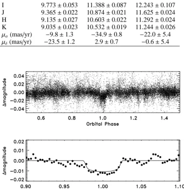
- WASP-57b was first observed in March 2008 and sub-sequently in Spring 2010. A total of 30172 points were taken of which about 855 were during transit. About 65 full or par-tial transits were observed overall with a ∆χ2 =
−151, and
S Nred = −6.20. Figure 3-upper panel shows the combined WASP light curves folded on the detected orbital period of 2.84 days. Additionally, for WASP-57b there is photometric coverage from the Qatar Exoplanet Survey (QES, Alsubai et al. 2011) and the phase folded QES light curve is shown in Figure 3-middle panel. In both WASP and QES light curves the tran-sit signal was identified with a period ∼2.84 days, duration
T14∼ 138 mins, and transit depth of ∼ 17 mmag.
Table 1. Photometric properties of the stars 54,
WASP-56 and WASP-57. The broad-band magnitudes and proper mo-tion are obtained from the NOMAD 1.0 catalogue.
Parameter WASP-54 WASP-56 WASP-57
RA(J2000) 13:41:49.02 12:13:27.90 14:55:16.84 Dec(J2000) −00:07:41.0 +23:03:20.2 −02:03:27.5 B 10.98± 0.07 12.74± 0.28 13.6± 0.5 V 10.42± 0.06 11.484± 0.115 13.04± 0.25 R 10.0± 0.3 10.7± 0.3 12.7± 0.3 I 9.773± 0.053 11.388± 0.087 12.243± 0.107 J 9.365± 0.022 10.874± 0.021 11.625± 0.024 H 9.135± 0.027 10.603± 0.022 11.292± 0.024 K 9.035± 0.023 10.532± 0.019 11.244± 0.026 µα(mas/yr) −9.8 ± 1.3 −34.9 ± 0.8 −22.0 ± 5.4 µδ(mas/yr) −23.5 ± 1.2 2.9± 0.7 −0.6 ± 5.4
Fig. 1. Upper panel: Discovery light curve of WASP-54b phase
folded on the ephemeris given in Table 4. Lower panel: binned WASP-54b light curve. Black-solid line, is the best-fit tran-sit model estimated using the formalism from Mandel & Agol (2002).
2.2. Low S/N photometry
Several observing facilities are available to the WASP consor-tium and are generally used to obtain multi-band low-resolution photometry to confirm the presence of the transit signal detected in the WASP light curves. This is particularly useful in case of unreliable ephemerides, and in case the transit period is such that follow up from a particular site is more challenging. Small-to-medium sized telescopes such as the remote-controlled 17-inch PIRATE telescope in the Observatori Astronomic de Mallorca (Holmes et al. 2011), together with the James Gregory 0.94 m telescope (JGT) at the University of St. Andrews, provide higher precision, higher spatial resolution photometry as compared to WASP, and thus have an important role as a link in the planet-finding chain, reducing the amount of large telescope time spent on false-positives. Observations of WASP-56 were obtained with both PIRATE and JGT, while observations of WASP-54 were obtained only with PIRATE.
Multiple Markov-Chain Monte Carlo (MCMC) chains have been obtained for both systems to assess the significance of adding the PIRATE and JGT light curves to the corresponding dataset in determining the transit model, in particular the impact parameter, the transit duration, and a/R⋆. We conclude that for
Fig. 2. Upper panel: Discovery light curve of WASP-56b phase
folded on the ephemeris given in Table 5. Lower panel: binned WASP-56b light curve. Black-solid line, is the best-fit tran-sit model estimated using the formalism from Mandel & Agol (2002).
WASP-54 the effect is not significant, never the less, the PIRATE light curves were included in our final analysis presented in sec-tion§3.2. In the case of WASP-56 instead, because we only have a partial TRAPPIST light curve (see section§2.4), the full JGT light curve, although of lower quality, is crucial to better con-strain the transit ingress/egress time, impact parameter and a/R⋆, allowing us to relax the main sequence mass-radius constraint.
2.3. Spectroscopic follow up
WASP-54, 56 and 57 were observed during our follow up cam-paign in Spring 2011 with the SOPHIE spectrograph mounted at the 1.93 m telescope (Perruchot et al. 2008; Bouchy et al. 2009) at Observatoire de Haute-Provence (OHP), and the CORALIE spectrograph mounted at the 1.2 m Euler-Swiss telescope at La Silla, Chile (Baranne et al. 1996; Queloz et al. 2000; Pepe et al. 2002). We used SOPHIE in high efficiency mode (R = 40 000) and obtained observations with very similar signal-to-noise ratio (∼30), in order to minimise systematic errors (e.g., the Charge Transfer Inefficiency effect of the CCD, Bouchy et al. 2009). Wavelength calibration with a Thorium-Argon lamp was per-formed every∼2 hours, allowing the interpolation of the spectral drift of SOPHIE (< 3 m s−1 per hour; see Boisse et al. 2010). Two 3′′diameter optical fibers were used; the first centered on the target and the second on the sky to simultaneously measure the background to remove contamination from scattered moon-light. During SOPHIE observations of WASP-54, 56 and 57 the contribution from scattered moonlight was negligible as it was well shifted from the targets’ radial velocities. The CORALIE observations of WASP-54 and WASP-57 were obtained during dark/grey time to minimise moonlight contamination. The data were processed with the SOPHIE and CORALIE standard data
Fig. 3. Upper panel: Discovery WASP light curve of WASP-57b
phase folded on the ephemeris given in Table 5. Middle panel: QES light curve of WASP-57b. Lower panel: binned WASP light curve of WASP-57b. Black-solid line, is the best-fit transit model estimated using the formalism from Mandel & Agol (2002).
reduction pipelines, respectively. The radial velocity uncertain-ties were evaluated including known systematics such as guiding and centering errors (Boisse et al. 2010), and wavelength cali-bration uncertainties. All spectra were single-lined.
For each planetary system the radial velocities were com-puted from a weighted cross-correlation of each spectrum with a numerical mask of spectral type G2, as described in Baranne et al. (1996) and Pepe et al. (2002). To test for possible stellar impostors we performed the cross-correlation with masks of different stellar spectral types (e.g. F0, K5 and M5). For each mask we obtained similar radial velocity variations, thus reject-ing a blended eclipsreject-ing system of stars with unequal masses as a possible cause of the variation.
We present in Tables 6, 7, and 8 the spectroscopic measure-ments of WASP-54, 56 and 57 together with their line bisec-tors (Vspan). In each Table we list the Barycentric Julian date (BJD), the stellar radial velocities (RVs), their uncertainties, the bisector span measurements, and the instrument used. In col-umn 6, we list the radial velocity measurements after subtract-ing the zero point offset to CORALIE and SOPHIE data respec-tively (the zero-point offsets are listed in Table 4, and Table 5 respectively). In column 7 we also give the line bisectors af-ter subtracting the mean value for SOPHIE and CORALIE re-spectively, and finally, in column 8, the radial velocity residuals to the best-fit Keplerian model. The Root-Mean-Square (RMS ) of the residuals to the best-fit Keplerian models are as follow:
RMS = 18.9 ms−1for WASP-54, RMS = 19.5 ms−1for WASP-56, and RMS = 24.4ms−1for WASP-57.
For all Figures presented in the paper we adopted the con-vention for which SOPHIE data are always represented as filled circles and CORALIE data are represented as open squares. In Figures 4 to 9 we present the RVs, Vspan, and the residuals O – C diagrams for the three systems. Both CORALIE and
Fig. 4. Upper panel: Phase folded radial velocity
measure-ments of WASP-54 obtained combining data from SOPHIE (filled-circles) and CORALIE (open-squares) spectrographs. Superimposed is the best-fit model RV curve with parameters from Table 4. The centre-of-mass velocity for each data set was subtracted from the RVs (γSOPHIE= -3.1109 km s−1 and
γCORALIE= -3.1335 km s−1). Lower panel: Residuals from the RV orbital fit plotted against time.
SOPHIE data sets are offset with respect to the radial velocity zero point, γSOPHIEand γCORALIE, respectively (see Tables 4 and 5). We examined Vspan to search for asymmetries in spectral line profiles that could result from unresolved binarity or indeed stellar activity. Such effects would cause the bisector spans to vary in phase with radial velocity. For the three systems no significant correlation is observed between the radial velocity and the line bisector, or the bisector and the time at which observation were taken. This supports each signal’s origin as being planetary, rather than due to a blended eclipsing binary system, or to stellar activity (see Queloz et al. 2001).
- WASP-54’s follow up spectroscopy was obtained from both the SOPHIE and CORALIE spectrographs (see Figures 4 and 5). The RMS for SOPHIE and CORALIE radial velocity resid-uals to the best-fit model are RMSSOPHIE = 33.6 m s−1 and
RMSCORALIE= 8.2 m s−1. Typical internal errors for CORALIE and SOPHIE are of 10–15 m s−1. The significantly higher RMS of the SOPHIE residuals is mostly due to one observation (RV = 134 m s−1). Removing this measurement results in a RMSSOPHIE
= 18 m s−1, which is comparable to the quoted internal error. We investigated the reasons of the particularly large error bar asso-ciated with the measurement above (55 m s−1) and we found that it is due to a shorter exposure time, cloud absorption, and Moon pollution. The specific observation was obtained during grey time at a Moon distance of 57◦. To estimate and remove the sky contamination we used the method described in Pollacco et al. (2008) and H´ebrard et al. (2008), however, the RV shift induced by the Moon was high (310 m s−1) and the relative low S/N
Fig. 5. Upper panel: The bisector span measurements of
WASP-54 as a function of radial velocity, values are shifted to a zero-mean (<Vspan>S OPHIE=−29 m s−1, <Vspan>CORALIE= 48 m s−1).
Lower panel: The bisector span measurements as a function of
time (BJD – 245 0000.0). The bisector span shows no significant variation nor correlation with the RVs, suggesting that the signal is mainly due to Doppler shifts of the stellar lines rather than stel-lar profile variations due to stelstel-lar activity or a blended eclipsing binary.
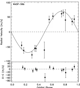
Fig. 6. Upper panel: Similar to Figure 4, the phase folded
ra-dial velocity measurements of WASP-56. The centre-of-mass velocity for the SOPHIE data was subtracted from the RVs (γSOPHIE= −4.6816 km s−1). Lower panel: Residuals from the RV orbital fit plotted against time.
Fig. 7. Upper panel: The bisector span measurements for
WASP-56 as a function of radial velocity, values are shifted to a zero-mean (<Vspan>S OPHIE= −40 m s−1). Lower panel: The bisector span measurements as a function of time (BJD – 245 0000.0). No correlation with radial velocity and time is ob-served suggesting that the Doppler signal is induced by the planet.
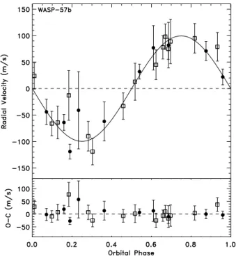
Fig. 8. Upper panel: Similar to Figures 4 and 6 for
WASP-57. The centre-of-mass velocity for each data set was sub-tracted from the RVs (γSOPHIE=−23.214 km s−1and γCORALIE=
−23.228 km s−1). Lower panel: Residuals from the RV orbital fit plotted against time.
Fig. 9. Upper panel: Same as Figures 5 and 7 we show the
bi-sector span measurements for WASP-57 as a function of ra-dial velocity, values are shifted to a zero-mean(<Vspan>S OPHIE= −2 m s−1, <V
span>CORALIE= 22 m s−1). Lower panel: The bisec-tor span measurements as a function of time (BJD – 245 0000.0). No correlation with radial velocity and time is observed suggest-ing that the Doppler signal is induced by the planet.
resulted in a less accurate measurement (1.3-σ away from the residuals).
- WASP-56 has radial velocity data only from SOPHIE (see Figures 6 and 7). The RMS of the RV residuals to the best-fit model is 19.4 m s−1. When removing the only discrepant RV value at phase 0.5 (RV =−61 m s−1) the overall RMS reduces to 12 m s−1, comparable to SOPHIE internal error. - Finally, for
WASP-57 the RMS of the SOPHIE and CORALIE radial
veloc-ity residuals to the best-fit model are RMSSOPHIE = 22.3 m s−1 and RMSCORALIE = 26.5 m s−1, respectively (see Figures 8 and 9). These become 14 m s−1and 17.4 m s−1respectively for SOPHIE and CORALIE data sets when ignoring the two mea-surements with the largest errors.
2.4. follow up Multi-band Photometry
In order to allow more accurate light curve modelling of the three new WASP planets and tightly constrain their param-eters, in-transit high-precision photometry was obtained with the TRAPPIST and Euler telescopes located at ESO La Silla Observatory in Chile. The TRAPPIST telescope and its char-acteristics are described in Jehin et al. (2011) and Gillon et al. (2011). A detailed description of the physical characteristics and instrumental details of EulerCam can be found in Lendl et al. (2012).
All photometric data presented here are available from the NStED database2. One full and one partial transits of WASP-54b have been observed by EulerCam in 2011 April 6 and TRAPPIST in 2012 February 26, respectively. Only a partial
Fig. 10. Euler r−band and TRAPPIST ‘I + z′−band follow up high signal-to-noise photometry of WASP-54 during the transit (see Table 2). The TRAPPIST light curve has been offset from zero by an arbitrary amount for clarity. The data are phase-folded on the ephemeris from Table 4. Superimposed (black-solid line) is our best-fit transit model estimated using the formalism from Mandel & Agol (2002). Residuals from the fit are displayed un-derneath.
Table 2. Photometry for WASP-54, WASP-56 and WASP-57
Planet Date Instrument Filter Comment
WASP-54b 06/04/2011 EulerCam Gunn r full transit 27/02/2012 TRAPPIST I + z partial transit WASP-56b 16/05/2011 TRAPPIST I + z partial transit
11/03/2012 JGT R full transit
WASP-57b
05/05/2011 TRAPPIST I + z partial transit 10/06/2011 TRAPPIST I + z full transit 10/06/2011 EulerCam Gunn r full transit
transit of WASP-56b was observed by TRAPPIST in 2011 May 16, and a full transit was observed by JGT in 2012 March 11. A partial and a full transit of WASP-57b were captured by TRAPPIST on the nights of 2011 May 5 and June 10 re-spectively, while a full transit of WASP-57b was observed with EulerCam in 2011 June 10. A summary of these observations is given in Table 2.
We show in Figures 10, 11, and 12 the high S/N follow up photometry (EulerCam and TRAPPIST) for 54b, WASP-56b and WASP-57b respectively. In each plot we show the differ-ential magnitude versus orbital phase, along with the residual to the best-fit model. The data are phase folded on the ephemerides derived by our analysis of each individual object (see§ 3.2). In Figures 10 and 12 some of the light curves are assigned an arbi-trary magnitude offset for clarity.
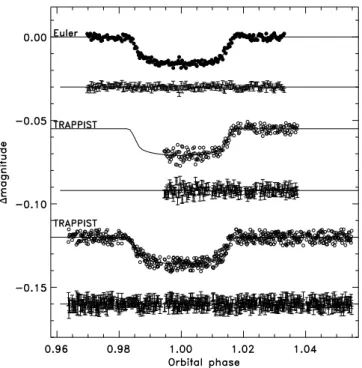
Fig. 11. TRAPPIST ‘I +z′−band and JGT R-band follow up high
signal-to-noise photometry of WASP-56 during the transit (see Table 2). The JGT light curve has been offset from zero by an arbitrary amount for clarity. The The data are phase-folded on the ephemeris from Table 5. Superimposed (black-solid line) is our best-fit transit model estimated using the formalism from Mandel & Agol (2002). Residuals from the fit are displayed un-derneath.
2.5. TRAPPIST ‘I + z’–band photometry
TRAPPIST photometry was obtained using a readout mode of 2× 2 MHz with 1 × 1 binning, resulting in a readout time of 6.1 s and readout noise 13.5 e−pix−1, respectively. A slight defo-cus was applied to the telescope to optimise the observation effi-ciency and to minimise pixel to pixel effects. TRAPPIST uses a special ‘I+z’ filter that has a transmittance > 90% from 750 nm to beyond 1100 nm. The positions of the stars on the chip were maintained to within a few pixels thanks to the ‘software guid-ing’ system that regularly derives an astrometric solution to the most recently acquired image and sends pointing corrections to the mount, if needed (see e.g., Gillon et al. 2011 for more de-tails). A standard pre-reduction (bias, dark, flat field correction), was carried out and the stellar fluxes were extracted from the images using the IRAF/DAOPHOT3 aperture photometry soft-ware Stetson (1987). After a careful selection of reference stars differential photometry was then obtained.
2.6. Euler r–band photometry
Observations with the Euler-Swiss telescope were obtained in the Gunn r filter. The Euler telescope employs an absolute track-ing system which keeps the star on the same pixel durtrack-ing the observation, by matching the point sources in each image with a catalogue, and adjusting the telescope pointing between expo-3 IRAF is distributed by the National Optical Astronomy
Observatory, which is operated by the Association of Universities for Research in Astronomy, Inc., under cooperative agreement with the National Science Foundation.
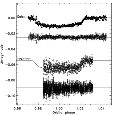
Fig. 12. Euler r−band and TRAPPIST ‘I + z′−band follow up high signal-to-noise photometry of WASP-57 during the tran-sit (see Table 2). The TRAPPIST light curves have been offset from zero by an arbitrary amount for clarity. The data are phase-folded on the ephemeris from Table 5. Superimposed (black-solid lines) are the best-fit transit models estimated using the for-malism from Mandel & Agol (2002). The residuals from each fit are displayed underneath the relative light curves.
sures to compensate for drifts (Lendl et al. 2012). WASP-54b’s observations were carried out with a 0.2 mm defocus and one-port readout with exposure time of 30 s. All images were cor-rected for bias and flat field effects and transit light curve were obtained by performing relative aperture photometry of the tar-get and optimal bright reference stars. For WASP-57b no defo-cus was applied, and observations were performed with four-port readout, and 60 s exposures. Six reference stars were used to per-form relative aperture photometry to obtain the final light curve.
3. Results
3.1. Stellar parameters
For all the three systems the same stellar spectral analysis has been performed, co-adding individual CORALIE and SOPHIE spectra with a typical final S/N of∼80:1. The standard pipeline reduction products were used in the analysis, and the analysis was performed using the methods given in Gillon et al. (2009). The Hα line was used to determine the effective temperature (Teff). The surface gravity (log g) was determined from the Ca i lines at 6122Å, 6162Å and 6439Å along with the Na i D and Mg i b lines. The elemental abundances were determined from equivalent width measurements of several clean and unblended lines. A value for micro-turbulence (ξt) was determined from Fe i using the method of Magain (1984). The quoted error estimates include that given by the uncertainties in Teff, log g and ξt, as well as the scatter due to measurement and atomic data uncertainties. The projected stellar rotation velocity (v sin i⋆) was determined by fitting the profiles of several unblended Fe i
lines. For each system a value for macro-turbulence (vmac) was assumed based on the tabulation by Bruntt et al. (2010), and we used the telluric lines around 6300Å to determine the instrumen-tal FWHM. The values for the vmacand the instrumental FWHM are given in Table 3. There are no emission peaks evident in the Ca H+K lines in the spectra of the three planet host stars. For each stellar host the parameters obtained from the analysis are listed in Table 3 and discussed below:
WASP-54: Our spectral analysis yields the following
results: Teff = 6100± 100 K, log g = 4.2 ± 0.1 (cgs), and [Fe/H]= −0.27 ± 0.08 dex, from which we estimate a spectral type F9. WASP-54’s stellar mass and radius were estimated using the calibration of Torres et al. (2010). We find no sig-nificant detection of lithium in the spectrum of WASP-54, with an equivalent width upper limit of 0.4 mÅ, corresponding to an abundance upper limit of log A(Li) < 0.4 ± 0.08. The non-detection of lithium together with the low rotation rate obtained from v sin i⋆(Prot = 17.60± 4.38 d), assuming i⋆ is perpendicular to the line of sight (thus v sin i⋆=V
equatorial), and the lack of stellar activity (shown by the absence of Ca ii H and K emission), all indicate that the star is relatively old. From the estimated v sin i⋆ we derived the stellar rotation rates, and we used the expected spin-down timescale (Barnes 2007) to obtain a value of the stellar age through gyrochronology. We estimate an age of 4.4+7.4−2.7 Gyr, This value also suggest the system is old. Although we point out that in the case of WASP-54 using gyrochoronlogy to constrain the age of the system could be in-appropriate as the planet could have affected the stellar rotation velocity via tidal interaction (see section§4.1 for more details). However, we note that the gyrochronological age we obtain is in agreement with that from theoretical evolutionary models discussed below, which imply that WASP-54 has evolved off the main sequence.
WASP-56 and WASP-57: Both stellar hosts are of spectral
type G6V. From our spectral analysis we obtain the following parameters: Teff = 5600± 100 K, and log g = 4.45 ± 0.1 (cgs) for WASP-56, Teff = 5600± 100 K, and log g = 4.2 ± 0.1 (cgs) for WASP-57. As before the stellar masses and radii are esti-mated using the Torres et al. (2010) calibration. With a metal-licity of [Fe/H]= 0.12 dex WASP-56 is more metal rich than the sun, while our spectral synthesis results for WASP-57 show that it is a metal poor star ([Fe/H]= −0.25 dex). For both stars the quoted lithium abundances take account non-local thermody-namic equilibrium corrections (Carlsson et al. 1994). The values for the lithium abundances if these corrections are neglected are as follows: log A(Li) = 1.32 and log A(Li) = 1.82 for WASP-56 and WASP-57, respectively. These values imply an age of >
∼ 5 Gyr for the former and an age of >∼ 2 Gyr for the latter (Sestito & Randich 2005). From v sin i⋆ we derived the stellar rotation period Prot = 32.58± 18.51 d for WASP-56, imply-ing a gyrochronological age (Barnes 2007) for the system of ∼ 5.5+10.6
−4.6 Gyr. Unfortunately, the gyrochronological age can only provide a weak constraint on the age of WASP-56. For WASP-57 we obtain a rotation period of Prot = 18.20± 6.40 d corresponding to an age of∼ 1.9+2.4−1.2Gyr. Both the above results are in agreement with the stellar ages obtained from theoretical evolution models (see below) and suggest that WASP-56 is quite old, while WASP-57 is a relatively young system.
For each system we used the stellar densities ρ⋆, measured directly from our Markov-Chain Monte Carlo (MCMC) anal-ysis (see §3.2, and also Seager & Mall´en-Ornelas 2003),
to-Fig. 13. Isochrone tracks from Marigo et al. (2008) and
Girardi et al. (2010) for WASP-54 using the metallicity [Fe/H]= −0.27 dex from our spectral analysis and the best-fit stellar den-sity 0.2 ρ⊙. From left to right the solid lines are for isochrones of: 1.0, 1.3, 1.6, 2.0, 2.5, 3.2, 4.0, 5.0, 6.3, 7.9, 10.0 and 12.6 Gyr. From left to right, dashed lines are for mass tracks of: 1.4, 1.3, 1.2, 1.1 and 1.0 M⊙.
Fig. 14. Isochrone tracks from Demarque et al. (2004) for
WASP-56 using the metallicity [Fe/H]= 0.12 dex from our spec-tral analysis and the best-fit stellar density 0.88 ρ⊙. From left to right the solid lines are for isochrones of: 1.8, 2.0, 2.5, 3.0, 4.0, 5.0, 6.0, 7.0, 8.0, 9.0, 10.0, 11.0, 12.0, 13.0 and 14.0 Gyr. From left to right, dashed lines are for mass tracks of: 1.2, 1.1, 1.0, 0.9 and 0.8 M⊙.
Table 3. Stellar parameters of 54, 56, and
WASP-57 from spectroscopic analysis.
Parameter WASP-54 WASP-56 WASP-57
Teff(K) 6100± 100 5600± 100 5600± 100 log g 4.2± 0.1 4.45± 0.1 4.2± 0.1 ξt(km s−1) 1.4± 0.2 0.9± 0.1 0.7± 0.2 v sin i⋆(km s−1) 4.0± 0.8 1.5± 0.9 3.7± 1.3 [Fe/H] −0.27 ± 0.08 0.12± 0.06 −0.25 ± 0.10 [Na/H] −0.30 ± 0.04 0.32± 0.14 −0.20 ± 0.07 [Mg/H] −0.21 ± 0.05 0.24± 0.06 −0.19 ± 0.07 [Si/H] −0.16 ± 0.05 0.31± 0.07 −0.13 ± 0.08 [Ca/H] −0.15 ± 0.12 0.09± 0.12 −0.21 ± 0.11 [Sc/H] −0.06 ± 0.05 0.35± 0.13 −0.08 ± 0.05 [Ti/H] −0.16 ± 0.12 0.18± 0.06 −0.18 ± 0.07 [Cr/H] −0.21 ± 0.12 0.20± 0.11 – [Co/H] – 0.35± 0.10 – [Ni/H] −0.29 ± 0.08 0.21± 0.07 −0.25 ± 0.10 log A(Li) <0.4± 0.08 1.37± 0.10 1.87± 0.10 Mass (M⊙) 1.15± 0.09 1.03± 0.07 1.01± 0.08 Radius (R⊙) 1.40± 0.19 0.99± 0.13 1.32± 0.18 Sp. Type F9 G6 G6 Distance (pc) 200± 30 255± 40 455± 80
Note: Mass and radius estimate using the Torres et al. (2010) calibra-tion. Spectral type estimated from Teffusing the table in Gray (2008).
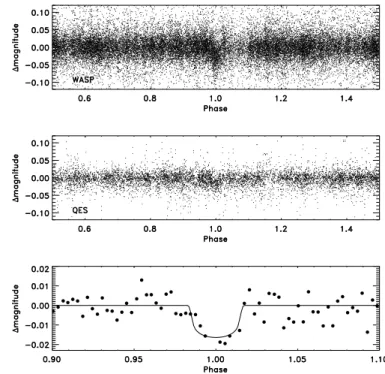
Fig. 15. Isochrone tracks from Demarque et al. (2004) for
WASP-57 using the metallicity [Fe/H]= −0.25 dex from our spectral analysis and the best-fit stellar density 1.638 ρ⊙. From left to right the solid lines are for isochrones of: 0.1, 0.6, 1.0, 1.6, 2.0, 2.5, 3.0, 4.0, 5.0 and 6.0 Gyr. From left to right, dashed lines are for mass tracks of: 1.1, 1.0, 0.9 and 0.8 M⊙.
gether with the stellar temperatures and metallicity values de-rived from spectroscopy, in an interpolation of four different stellar evolutionary models. The stellar density, ρ⋆, is directly determined from transit light curves and as such is indepen-dent of the effective temperature determined from the spectrum (Hebb et al. 2009), as well as of theoretical stellar models (if
Mpl ≪ M⋆is assumed). Four theoretical models were used: a) the Padova stellar models (Marigo et al. 2008, and Girardi et al. 2010), b) the Yonsei-Yale (YY) models (Demarque et al. 2004), c) the Teramo models (Pietrinferni et al. 2004) and finally d) the Victoria-Regina stellar models (VRSS) (VandenBerg et al. 2006). In Figures 13, 14, and 15, we plot the inverse cube root of the stellar density ρ⋆−1/3= R⋆/M⋆1/3(solar units) against ef-fective temperature, Teff, for the selected model mass tracks and isochrones, and for the three planet host stars respectively. For WASP-54 and WASP-56 the stellar properties derived from the four sets of stellar evolution models (Table 9) agree with each other and with those derived from the Torres et al. (2010) cali-bration, within their 1–σ uncertainties. For WASP-57 the best-fit M⋆ from our MCMC analysis agrees with the values de-rived from theoretical stellar tracks with the exception of the Teramo models. The latter give a lower stellar mass value of 0.87± 0.04 M⊙which is more than 1–σ away from our best-fit result (although within 2–σ). The stellar masses of planet host stars are usually derived by comparing measurable stel-lar properties to theoretical evolutionary models, or from em-pirical calibrations. Of the latter, the most widely used is the Torres et al. (2010) calibration, which is derived from eclipsing binary stars, and relates log g and Teff to the stellar mass and radius. However, while Teff can be determined with high preci-sion, log g is usually poorly constrained, and thus stellar masses derived from the spectroscopic log g can have large uncertain-ties and can suffer from systematics. For example the masses of 1000 single stars, derived by Valenti et al. (1998) via spec-tral analysis, were found to be systematically 10% larger than those derived from theoretical isochrones. A similar discrep-ancy was also found in the analysis of the stellar parameters of WASP-37 (Simpson et al. 2011), WASP-39 (Faedi et al. 2011), and WASP-21 (Bouchy et al. 2010). Additionally, different sets of theoretical models might not perfectly agree with each other (Southworth 2010), and moreover at younger ages isochrones are closely packed and a small change in Teff or ρ⋆ can have a significant effect on the derived stellar age. For each planet host star we show a plot with one set of stellar tracks and isochrones, while we give a comprehensive list of the four models’ results in Table 9. Using the metallicity of [Fe/H]=−0.27 dex our best-fit stellar properties from the Padova isochrones (Marigo et al. 2008 and Girardi et al. 2010) for WASP-54 yield a mass of 1.1+0.1
1.0 M⊙and a stellar age of 6.3
+1.6
−2.4Gyr, in agreement with the gyrochronological age and a more accurate estimate. The Padova isochrones together with the stellar mass tracks and WASP-54 results are shown In Figure 13. According to the stellar models, a late-F star with [Fe/H]= −0.27 dex, of this radius and mass has evolved off the zero-age main sequence and is in the shell hydrogen burning phase of evolution with an age of 6.3+1.6
−2.4Gyr. The best-fit stellar ages from the other sets of stellar models of WASP-54 also agree with our conclusion. In Figure 13 the large uncertainty on the minimum stellar mass estimated from inter-polation of the Padova isochrones is likely due to the proximity to the end of the main sequence kink. The Padova evolutionary models were selected nevertheless, because they show clearly the evolved status of WASP-54.
In Figures 14, and 15 we show the best-fit Yonsei-Yale stellar evolution models and mass tracks (Demarque et al. 2004) for the planet host stars WASP-56 and WASP-57, respectively. Using the metallicity of [Fe/H]= 0.12 dex for WASP-56 our fit of the YY-isochrones gives a stellar mass of 1.01+0.03−0.04M⊙and a stellar age of 6.2+3.0−2.1Gyr. This is in agreement with the Li abundance measured in the spectral synthesis (see Table 3), and supports the conclusion that WASP-56 is indeed an old system. Using
the metallicity of [Fe/H]=−0.25 dex derived from our spectral analysis of WASP-57, we interpolate the YY-models and we ob-tain a best-fit stellar mass of 0.89+0.04
−0.03M⊙and age of 2.6 +2.2 −1.8Gyr. These results also agree with our results from spectral synthesis and shows that WASP-57 is a relatively young system. For each system the uncertainties in the derived stellar densities, temper-atures and metallicities were included in the error calculations for the stellar ages and masses, however systematic errors due to differences between various evolutionary models were not con-sidered.
3.2. Planetary parameters
The planetary properties were determined using a simultane-ous Markov-Chain Monte Carlo analysis including the WASP photometry, the follow up TRAPPIST and Euler photom-etry, together with SOPHIE and CORALIE radial velocity measurements (as appropriate see Table 2 and Tables 6, 7, and 8). A detailed description of the method is given in Collier Cameron et al. (2007) and Pollacco et al. (2008). Our it-erative fitting method uses the following parameters: the epoch of mid transit T0, the orbital period P, the fractional change of flux proportional to the ratio of stellar to planet surface areas ∆F = R2
pl/R 2
⋆, the transit duration T14, the impact parameter b, the radial velocity semi-amplitude K1, the stellar effective tem-perature Teff and metallicity [Fe/H], the Lagrangian elements
√
e cos ω and √e sin ω (where e is the eccentricity and ω the
longitude of periastron), and the systematic offset velocity γ. For WASP-54 and WASP-57 we fitted the two systematic ve-locities γCORALIE and γSOPHIE to allow for instrumental offsets between the two data sets. The sum of the χ2 for all input data curves with respect to the models was used as the goodness-of-fit statistic. For each planetary system four different sets of solutions were considered: with and without the main-sequence mass-radius constraint in the case of circular orbits and orbits with floating eccentricity.
An initial MCMC solution with a linear trend in the systemic velocity as a free parameter, was explored for the three plane-tary systems, however no significant variation was found. For the treatment of the stellar limb-darkening, the models of Claret (2000, 2004) were used in the r-band, for both WASP and Euler photometry, and in the z-band for TRAPPIST photometry.
From the parameters mentioned above, we calculate the mass M, radius R, density ρ, and surface gravity log g of the star (which we denote with subscript ⋆) and the planet (which we denote with subscriptpl), as well as the equilibrium temperature of the planet assuming it to be a black-body (Tpl,A=0) and that energy is efficiently redistributed from the planet’s day-side to its night-side. We also calculate the transit ingress/egress times
T12/T34, and the orbital semi-major axis a. These calculated values and their 1–σ uncertainties from our MCMC analysis are presented in Tables 4 and 5 for WASP-54, WASP-56 and WASP-57. The corresponding best-fitting transit light curves are shown in Figures 1, 2, and 3 and in Figures 10, 11, and 12. The best-fitting RV curves are presented in Figures 4, 6, and 8.
– For WASP-54 the MCMC solution imposing the main sequence mass-radius constraint gives unrealistic values for the best-fit stellar temperature and metallicity, as we expected for an evolved star. We then relaxed the main sequence constraint and explored two solutions: one for a circular and one for an eccentric orbit. In the case of a non-circular orbit we obtain a best-fit value for e of 0.067+0.033−0.025. This is less than a 3–σ
detection, and as suggested by Lucy & Sweeney (1971), Eq. 22, it could be spurious. From our analysis we obtain a best-fit χ2 statistic of χ2
circ = 24.3 for a circular orbit, and χ 2
ecc = 18.6 for an eccentric orbit. The circular model is parameterised by three parameters: K, γSOPHIE and γCORALIE, while the eccentric model additionally constrains e cos ω and e sin ω. We used the 23 RV measurements available and we performed the Lucy & Sweeney F-test (Eq. 27 of Lucy & Sweeney 1971), to investigate the probability of a truly eccentric orbit for WASP-54b. We obtained a probability of 9% that the improvement in the fit produced by the best-fitting eccentricity could have arisen by chance if the orbit were real circular. Lucy & Sweeney (1971) suggest a 5% probability threshold for the eccentricity to be significant. From our MCMC analysis we obtain a best-fit value for ω = 62+20−30 de-gree, this differs from 90 ◦ or 270◦ values expected from an eccentric fit of a truly circular orbit (see Laughlin et al. 2005). We decided to investigate further our chances to detect a truly eccentric orbit which we discuss in §3.3. Table 4 shows our best-fit MCMC solutions for WASP-54b for a forced circular orbit, and for an orbit with floating eccentricity. However, based on our analysis in§3.3, we adopted the eccentric solution.
– For WASP-56b the available follow up spectroscopic and photometric data do not offer convincing evidence for an eccentric orbit. The free-eccentricity MCMC solution yields a value of e = 0.098± 0.048. The Lucy & Sweeney (1971) F-test, indicates that there is a 42% probability that the improvement in the fit could have arisen by chance if the orbit were truly circular. With only a partial high S/N follow up light curve it is more difficult to precisely constrain the stellar and planetary parameters (e.g., the time of ingress/egress, the impact parame-ter b, and a/R⋆), however the full, although noisy, low S/N GJT light curve (see Figure 11), allows us to better constrain the parameters mentioned above. Therefore we decided to relax the main-sequence constrain on the stellar mass and radius and we adopt a circular orbit.
– For WASP-57b the follow up photometry and radial ve-locity data allowed us to relax the main-sequence mass-radius constrain and perform an MCMC analysis leaving the eccentric-ity as free parameter. However, our results do not show evidence for an eccentric orbit, and the Lucy & Sweeney test yields a 100% probability that the orbit is circular. Moreover, we find that imposing the main-sequence constraint has little effect on the MCMC global solution. Thus, we decided to adopt no main sequence prior and a circular orbit.
3.3. The Eccentricity of WASP-54b
Here we investigate possible biases in the detection of the ec-centricity of WASP-54b, and we explore the possibility that the eccentricity arises from the radial velocity measurements alone. It is well known that eccentricity measurements for a planet in a circular orbit can only overestimate the true zero eccentricity (Ford 2006). We want to quantify whether using only the radial velocity measurements at hand we can find a significant differ-ence in the best-fit model of truly circular orbit compared to that of a real eccentric orbit with e = 0.067, as suggested by our free-floating eccentric solution. Indeed, the best-fit eccentricity depends on the signal-to-noise of the data, on gaps in the phase coverage, on the number of orbital periods covered by the data set, and the number of observations (see e.g., Zakamska et al. 2011).
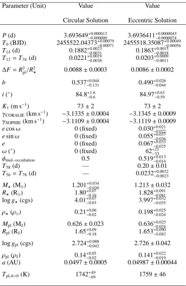
Table 4. System parameters of WASP-54
Parameter (Unit) Value Value
Circular Solution Eccentric Solution
P (d) 3.693649+0.000013 −0.000009 3.6936411 +0.0000043 −0.0000074 T0(BJD) 2455522.04373+0.00079−0.00071 2455518.35087+0.00049−0.00056 T14(d) 0.1882+0.0023−0.0031 0.1863+0.0015−0.0018 T12= T34(d) 0.0221+0.0019−0.0038 0.0203+0.0009−0.0011 ∆F = R2 pl/R 2 ⋆ 0.0088± 0.0003 0.0086± 0.0002 b 0.537+0.044 −0.131 0.490 +0.026 −0.044 i (◦) 84.8+1.6 −0.6 84.97 +0.63 −0.59 K1(m s−1) 73± 2 73± 2 γCORALIE(km s−1) −3.1335 ± 0.0004 −3.1345 ± 0.0009 γSOPHIE(km s−1) −3.1109 ± 0.0004 −3.1119 ± 0.0009 e cos ω 0 (fixed) 0.030+0.021 −0.022 e sin ω 0 (fixed) 0.055+0.037 −0.036 e 0 (fixed) 0.067+0.033 −0.025 ω(◦) 0 (fixed) 62+21 −33 φmid−occultation 0.5 0.519+0.013 −0.014 T58(d) — 0.20± 0.01 T56= T78(d) — 0.0232+0.0032−0.0023 M⋆(M⊙) 1.201+0.034−0.036 1.213± 0.032 R⋆(R⊙) 1.80+0.07−0.16 1.828 +0.091 −0.081 log g⋆(cgs) 4.01+0.07−0.03 3.997+0.032−0.035 ρ⋆(ρ⊙) 0.21+0.06−0.02 0.198 +0.025 −0.024 Mpl(MJ) 0.626± 0.023 0.636+0.025−0.024 Rpl(RJ) 1.65+0.09−0.18 1.653+0.090−0.083 log gpl(cgs) 2.724+0.088−0.042 2.726± 0.042 ρpl(ρJ) 0.14+0.05−0.02 0.141+0.022−0.019 a (AU) 0.0497± 0.0005 0.04987± 0.00044 Tpl,A=0(K) 1742+49−69 1759± 46 aT
14: time between 1stand 4thcontact
Notes. RJ/R⊙= 0.10273; MJ/M⊙=0.000955
We use the uncertainty of the CORALIE and SOPHIE radial velocity measurements of WASP-54, the MCMC best-fit orbital period, velocity semi-amplitude K, and epoch of the transit T0 as initial parameters, to compute synthetic stellar radial veloci-ties at each epoch of the actual WASP-54 RV data set. We gen-erated synthetic radial velocity data using the Keplerian model of Murray & Dermott (1999), for the two input eccentricities,
e = 0 and e = 0.067. We then added Gaussian noise deviates
to the synthetic RV at each epoch, corresponding to the original RV uncertainties added in quadrature with 3.5 m s−1accounting for stellar jitter. In this way at each observation time the simu-lated velocity is a random variable normally distributed around a value v(ti) + γ, with dispersion
q σ2
obs+ σ 2
Jitter, where γ is the centre of mass velocity. In this manner the simulated data have similar properties to the real WASP-54 velocities but with the advantage of having a known underlying eccentricity and orbital properties.
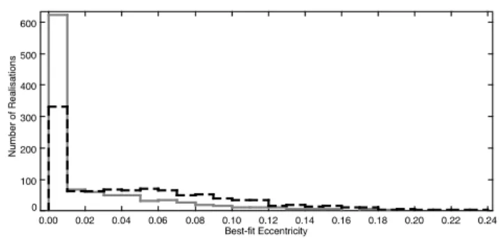
We generated 1000 synthetic data sets for each input eccen-tricity and found the best-fit values for e. In Figure 16 we show the output eccentricity distributions for the input e = 0 (grey solid line), and for the input eccentricity of 0.067 (black dashed
Table 5. System parameters of WASP-56 and WASP-57
WASP-56 WASP-57
Parameter (Unit) Value Value
P (d) 4.617101+0.000004 −0.000002 2.838971± 0.000002 T0(BJD) 2455730.799± 0.001 2455717.87811± 0.0002 T14(d) 0.1484± 0.0025 0.0960± 0.0005 T12= T34(d) 0.0146± 0.0005 0.01091+0.00032−0.00018 ∆F = R2 pl/R 2 ⋆ 0.01019± 0.00041 0.01269± 0.00014 b 0.272+0.029 −0.018 0.345 +0.033 −0.014 i (◦) 88.5+0.1 −0.2 88.0 +0.1 −0.2 K1(m s−1) 69± 4 100± 7 γSOPHIE(km s−1) 4.6816± 0.0001 −23.214 ± 0.002 γCORALIE(km s−1)) — −23.228 ± 0.002 e 0 (fixed) 0 (fixed) M⋆(M⊙) 1.017± 0.024 0.954± 0.027 R⋆(R⊙) 1.112+0.026−0.022 0.836 +0.07 −0.16 log g⋆(cgs) 4.35± 0.02 4.574+0.009−0.012 ρ⋆(ρ⊙) 0.74± 0.04 1.638+0.044−0.063 Mpl(MJ) 0.571+0.034−0.035 0.672+0.049−0.046 Rpl(RJ) 1.092+0.035−0.033 0.916+0.017−0.014 log gpl(cgs) 3.039+0.035−0.038 3.262+0.063−0.033 ρpl(ρJ) 0.438+0.048−0.046 0.873+0.076−0.071 a (AU) 0.05458± 0.00041 0.0386± 0.0004 Tpl,A=0(K) 1216+25−24 1251+21−22 aT
14: time between 1stand 4thcontact
Notes. RJ/R⊙= 0.10273; MJ/M⊙=0.000955
Fig. 16. Histograms of the output eccentricity distributions for
the input e = 0 (grey solid line), and for the input eccentricity of 0.067 (black dashed line).
line). Clearly, the one-dimensional distribution of the output ec-centricity is highly asymmetric. Because e is always a positive parameter, the best-fit eccentricities are always positive values. We used the 1000 output best-fit values of e of the two samples of synthetic data sets to perform the Kolmogorov-Smirnov (KS) test to asses our ability to distinguish between the two underlying distributions. In Figure 17 we show the Cumulative Distribution Function (CDFs) of the 1000 mock best-fit eccentricities for the two cases. We show in grey the CDFs for the simulated data sets with underlying circular orbits, and in black the CDFs for the eccentric case. We calculated D, the absolute value of the
Fig. 17. Cumulative Distribution Function for the two sets of
best-fit eccentricities. We show in grey the CDFs for the sim-ulated data sets with underline circular orbits, and in black the CDFs for the eccentric ones.
maximum difference between the CDFs of the two samples, and we used tabulated values for the KS test. We are able to reject the hypothesis that the two samples have the same underlying distribution with a confidence of 99.999%. We then conclude that the detected eccentricity of WASP-54b could indeed be real. We point out however, that time-correlated noise could poten-tially yield a spurious eccentricity detection. This is difficult to asses with the limited number of radial velocity observations at hand; more data and photometric monitoring during transit and secondary eclipses are needed to better constrain the orbital pa-rameters of WASP-54b. In the following, we adopt the eccentric MCMC model for WASP-54b.
4. Discussion
We report the discovery of three new transiting extra-solar plan-ets from the WASP survey, 54b, 56b and WASP-57b. In the following we discuss the implications of these new planet discoveries.
4.1. WASP-54b
From our best-fit eccentric model we obtain a planetary mass of 0.634+0.025
−0.024 MJ and a radius of 1.653 +0.090
−0.083 RJ which yields a planetary density of 0.141+0.022−0.019 ρJ. Thus, WASP-54b is among the least dense, most heavily bloated exoplanets and shares similarities with low-density planets such as WASP-17b (Anderson et al. 2010b), WASP-31b (Anderson et al. 2010a), and WASP-12b (Hebb et al. 2010). These exoplanets have short orbital periods, orbit F-type host stars and therefore are highly irradiated. Using standard coreless models from Fortney et al. (2007) and Baraffe et al. (2008), we find that WASP-54b has a radius more than 50% larger than the maximum planetary radius predicted for a slightly more massive 0.68MJ coreless planet, orbiting at 0.045 AU from a 5 Gyr solar-type star (Rexpected=1.105 RJ ). However, WASP-54 is an F-type star and therefore hotter than the Sun, implying that WASP-54b is more strongly irradiated. The low stellar metallicity ([Fe/H]= −0.27 ± 0.08) of WASP-54 supports the expected low plane-tary core-mass thus favouring radius inflation. Different mecha-nisms have been proposed to explain the observed anomalously
large planetary radii such as tidal heating (Bodenheimer et al. 2001, 2003), kinetic heating (Guillot & Showman 2002), en-hanced atmospheric opacity (Burrows et al. 2007), and semi-convection (Chabrier & Baraffe 2007). While each individual mechanism would presumably affect all hot Jupiters to some de-gree – for example the detected non-zero eccentricity of WASP-54b and the strong stellar irradiation are contributing to the radius inflation – they cannot explain the entirety of the ob-served radii (Fortney & Nettelmann 2010, Baraffe et al. 2010), and additional mechanisms are needed to explain the inflated radius of WASP-54b. More recently, Batygin et al. (2011) and Perna et al. (2010) showed that the ohmic heating mechanism (dependent on the planet’s magnetic field and atmospheric heavy element content), could provide a universal explanation of the currently measured radius anomalies (see also Laughlin et al. 2011). However, according to Wu & Lithwick (2012) Eq.6, the maximum expected radius for WASP-54b, including ohmic heat-ing, is 1.61RJ. This value for the radius is calculated assuming a system’s age of 1 Gyr and that ohmic heating has acted since the planet’s birth. Therefore, if we regard this value as an upper limit for the expected radius of WASP-54b at 6 Gyr, it appears more difficult to reconcile the observed anomalously large ra-dius of WASP-54b (although the value is within 1-σ) even when ohmic heating is considered, similarly to the case of WASP-17b (Anderson et al. 2010a), and HAT-P-32b (Hartman et al. 2011), as discussed by Wu & Lithwick (2012). Additionally, Huang & Cumming (2012) find that the efficacy of ohmic heat-ing is reduced at high Teff and that it is difficult to explain the observed radii of many hot Jupiters with ohmic heating under the influence of magnetic drag. The ability of ohmic heating in inflating planetary radii depends on how much power it can generate and at what depth, with deeper heating able to have a stronger effect on the planet’s evolution (Rauscher & Menou 2012; Guillot & Showman 2002). Huang & Cumming (2012) models predict a smaller radius for WASP-54b (see their Fig. 12).
However, the discrepancy between observations and the ohmic heating models in particular in the planetary low-mass regime (e.g. Batygin et al. 2011), shows that more understand-ing of planets’ internal structure, chemical composition and evo-lution is required to remove assumptions limiting current the-oretical models. Moreover, Wu & Lithwick (2012) suggest that ohmic heating can only suspend the cooling contraction of hot– Jupiters; planets that have contracted before becoming subject to strong irradiation, can not be re-inflated. Following this sce-nario, the observed planetary radii could be relics of their past dynamical histories. If this is true, we could expect planets mi-grating via planet–planet scattering and/or Kozai mechanisms (which can become important at later stages of planetary forma-tion compared to disc migraforma-tion, (Fabrycky & Tremaine 2007, Nagasawa et al. 2008), to show a smaller radius anomaly and large misalignments. This interesting possibility can be tested by planets with Rossiter-McLaughlin (RM) measurements of the spin–orbit alignment (Holt 1893; Rossiter 1924; McLaughlin 1924 Winn et al. 2006). We use all systems from the RM-encyclopedia (http://ooo.aip.de/People/rheller/) to estimate the degree of spin-orbit (mis)alignment. We consider aligned ev-ery system with |λ| < 30◦ (a 3–σ detection from zero de-grees; Winn et al. 2010), and define ηRM = (|λ| − 30◦)/30◦ as the measure of the degree of (mis)alignment of each system. This has the advantage to show all aligned systems in the re-gion−1 < ηRM ≤ 0. In Figure 18 we show ηRM versus the ra-dius anomaly and the stellar temperature Teff (as a colour gra-dient) for planets with RM measurements. We have calculated
Fig. 18. We plot the degree of (mis)alignment, ηRM, versus the
radius anomalyR and the stellar effective temperature for known planets (see text for details). The black dashed line separates aligned from mis-aligned systems following our description. The black solid line indicatesR = 0. Known planetary systems with characteristics across the parameter space are indicated as fol-lows: W for WASP, H for HatNet, C for CoRoT, K for Kepler, and others by their full name. Our three new discoveries are indi-cated by fuchsia square symbols. We note that no RM measure-ment is yet available for WASP-54b, WASP-56b, WASP-57b.
the radius anomaly, R, as follows (Robs− Rexp)/Rexp, see also Laughlin et al. (2011). We find it difficult to identify any corre-lation (see also Jackson et al. 2012, and their Fig. 11). We want to stress here that the uncertainty in the timescales of planet– planet scattering and Kozai migration mechanism relative to disc migration remain still large and thus any robust conclusion can not be drawn until all the underlying physic of migration is understood. Moreover, Albrecht et al. (2012) suggest that the Kozai mechanism is responsible for the migration of the ma-jority, if not all, hot Jupiters, those mis-aligned as well as the aligned ones, and finally, that tidal interaction plays a central role. Additionally, measurements of spin–orbit obliquities could bear information about the processes involved in star formation and disc evolution rather than on the planet migration. For exam-ple Bate et al. (2010) have recently proposed that stellar discs could become inclined as results of dynamics in their environ-ments (e.g. in stellar clusters), and Lai et al. (2011) suggest that discs could be primordially mis-aligned respect to the star, al-though Watson et al. (2011) could find no evidence of disc mis-alignment. Last but not least we note that not many planets show-ing the radius anomaly have measured RM effects and that more observations are needed to constrain theoretical models before any robust conclusion can be drawn.
We investigate the radius anomaly of WASP-54b with re-spect to the full sample of known exoplanets and rere-spect to the sample of Saturn-mass planets including the latest discoveries and the planets presented in this work (for an updated list see the extra-solar planet encyclopaedia4. In Figure 19 we plot the plan-etary radius versus the stellar metallicity (left panel), and as a function of the planet equilibrium temperature Teq(right panel). WASP-54b is indicated with a filled fuchsia circle. We highlight the sample of Saturn mass planets in turquoise; the black and turquoise dashed lines show a simple linear regression for the full exoplanet and the Saturn mass sample respectively.
WASP-54b appears to strengthen the correlation between planets’ inflated radii and stellar temperature, and the
Fig. 19. The Planetary radius versus stellar metallicity [Fe/H] (dex)(left panel), and as a function of planet equilibrium temperature
Teq (K) (right panel). Black points indicate all planets, planets in the mass range 0.2< Mpl <0.7MJ are indicated by Turquoise points. Black and turquoise dashed lines are a simple linear regression to the two samples. Data were taken from the exoplanet encyclopaedia. Known planetary systems with characteristics across the parameter space are indicated as in Figure 18. Our three new discoveries are indicated by fuchsia filled circles.
correlation with metallicity. With an irradiation temperature of ∼2470 K, WASP-54b is in the temperature region, identified by Perna et al. (2012), with Tirr > 2000 K (Tirr as defined by Heng et al. 2012), in which planets are expected to show large day-night flux contrast and possibly temperature inversion, in which case the ohmic power has its maximum effect. With more gas giant planet detections we can start to shed some light on which mechanism might be more efficient and in which cir-cumstances. For example, in the case of WASP-39b (Faedi et al. 2011), and WASP-13b (Skillen et al. 2009; Barros et al. 2011), two Saturn-mass planets with similar density to WASP-54b, but much less irradiated (Teq = 1116 K, and Teq = 1417 K, re-spectively) ohmic heating could play a less significant role (see for example Perna et al. 2012). However, many unknowns still remain in their model (e.g., internal structure, magnetic field strength, atmospheric composition). We selected all the exo-planets in the mass range between 0.1 < Mpl < 12MJ, and we used the empirical calibrations for planetary radii derived by Enoch et al. (2012) to calculate the expected planetary ra-dius Rexp. We then used these values to derive again the Radius Anomaly. We plot the results of radius anomaly versus stellar metallicity [Fe/H] and as a function of Teqin Figure 20. Colours and symbols are like in Figure 19, the dotted line indicates a zero radius anomaly. The Enoch et al. (2012) relations take into account the dependence of the planetary radius from planet Teq, [Fe/H], and also tidal heating and semi-major axis. However, we note that even including this dependence, there remained signif-icant scatter in the observed radii in particular for systems such as WASP-17b, WASP-21b and also WASP-54b, WASP-56b and WASP-57b.
Thus, more gas giant planet discoveries and their accurate characterisation are needed to compare planetary physical prop-erties, in order to understand their thermal structure and distin-guish between various theoretical models. With a magnitude of V= 10.42 WASP-54 is a bright target and thus its spectroscopic and photometric characterisation is readily feasible. Given the detected non-zero eccentricity we encourage secondary eclipse observations in the IR. These observations will allow precise measurement of the system’s eccentricity as well as provide
fundamental information on the thermal structure of the planet. However, we note that even in the case of a circular orbit our MCMC solution for WASP-54 yields a very similar, inflated, planetary radius Rcircpl = 1.65 RJ, see Table 4.
Finally, WASP-54 is an old (> 6 Gyr) F9 star which has evolved off the main sequence and is now in the Hydrogen shell-burning phase of stellar evolution (see Figure 13). This implies that recently in its life WASP-54 has increased its radius by more than 60%, and thus it is ascending the red giant branch (RGB). WASP-54b thus could be experiencing drag forces, both gravita-tional and tidal, which will affect its orbital radius. Two main factors contribute to the change of the planetary orbit: 1) the host-star can lose mass via stellar wind which could be accreted by the planet resulting in an increase of the orbital radius, and 2) the planet’s orbital angular momentum decreases due to the tidal drag, leading to a decrease of the orbital radius. This is expressed by ˙apl = ˙atide+ ˙amass loss(Zahn 1977, 1989). While the second term is negligible for Jupiter-like planets (Duncan & Lissauer 1998), the term due to tides can become important as it is pro-portional to (R⋆/a(r))8, where a(r) is the decreasing orbital ra-dius. This could re-set the clock of WASP-54b making it appear younger, and maybe contributing to the planet radius inflation. Finally, any planet within the reach of the star’s radius during RGB and asymptotic giant branch (AGB) phases (about 1 AU for a Solar-type star) will spiral-in and eventually merge with the star or evaporate (Villaver & Livio 2007; Livio & Soker 1984).
4.2. WASP-56b and WASP-57b
Our modelling of the WASP-56 system yields a planet mass of 0.571+0.034
−0.035 MJ and radius of 1.092 +0.035
−0.033RJ which in turn give a planet density of 0.438+0.048−0.046 ρJ. Hence WASP-56b belongs to the class of Saturn-mass planets and does not show a radius anomaly (Laughlin et al. 2011). Figure 19 shows that the radius of WASP-56b is not inflated. With a metallicity of [Fe/H]= +0.12 dex WASP-56 is more metal rich than the Sun, and with an age of ∼6.3 Gyr standard planetary evolutionary models from Fortney et al. (2007) and Baraffe et al. (2008), show that WASP-56b has a core of approximately > 10 M⊕ of heavy
![Fig. 15. Isochrone tracks from Demarque et al. (2004) for WASP-57 using the metallicity [Fe/H]= − 0.25 dex from our spectral analysis and the best-fit stellar density 1.638 ρ ⊙](https://thumb-eu.123doks.com/thumbv2/123doknet/5477736.130165/9.892.66.451.611.1004/isochrone-tracks-demarque-metallicity-spectral-analysis-stellar-density.webp)