HAL Id: hal-01561628
https://hal-mines-paristech.archives-ouvertes.fr/hal-01561628
Submitted on 13 Jul 2017
HAL is a multi-disciplinary open access
archive for the deposit and dissemination of sci-entific research documents, whether they are pub-lished or not. The documents may come from teaching and research institutions in France or abroad, or from public or private research centers.
L’archive ouverte pluridisciplinaire HAL, est destinée au dépôt et à la diffusion de documents scientifiques de niveau recherche, publiés ou non, émanant des établissements d’enseignement et de recherche français ou étrangers, des laboratoires publics ou privés.
Simulations
Kristian Pagh Nielsena, Philippe Blanc, Franck Vignola, Lourdes Ramirez,
Manuel Blanco, Richard Meyer
To cite this version:
Kristian Pagh Nielsena, Philippe Blanc, Franck Vignola, Lourdes Ramirez, Manuel Blanco, et al.. Discussion of currently used practices for: ”Creation of Meteorological Data Sets for CSP/STE Per-formance Simulations. [Research Report] SolarPACES Report, IEA SolarPACES. 2017, 103 p. �hal-01561628�
Page 1 of 103
Discussion of currently used practices for:
“Creation of Meteorological Data Sets for
CSP/STE Performance Simulations”
Kristian Pagh Nielsena, Philippe Blancb, Frank Vignolac, Lourdes Ramírezd, Manuel Blancoe, Richard Meyerf
a
Danish Meteorological Institute, DK-2100 Copenhagen, Denmark. b
ARMINES, F-75272 Paris Cedex 06, France. c
The Solar Radiation Monitoring Lab, University of Oregon, Eugene, OR 97403-1274, USA.
d
CIEMAT, E-28040, Madrid, Spain. e
The Cyprus Institute, Athalassa Campus, 20 Konstantinou Kavafi Street 2121, Aglantzia, Nicosia, Cyprus.
f
Page 2 of 103
Introduction
A Concentrating Solar Power (CSP)/Solar Thermal Electric (STE) power plant is a substantial long-term investment. To evaluate the opportunities and risks associated with such a long-long-term in-vestment requires careful technical and economic analysis. Usually, the results of such analysis are presented in what are known as feasibility studies.
Traditional CSP/STE feasibility studies start by defining an economic model to estimate the eco-nomic metrics that characterize the quality and attractiveness of the investment project associat-ed with the building and exploitation of the CSP/STE power plant. Typical economic metrics are the Levelized Cost of Energy (LCOE), the Internal Rate of Return (IRR), the Net Present Value (NPV), and the Debt Coverage Ratio (DCR).
Once the model is defined, the main challenge is to accurately estimate the technical and econom-ic variables and parameters that informs the model (see Figure 1), such as the project’s Total In-vestment, the Annual O&M costs, the Annual Electricity Generation, the Discount Rates, the Equi-ty-to-Debt ratio, etc.
Figure 1. Traditional feasibility study approach.
Of all of these variables and parameters, the Annual Electricity Generation is the one that charac-terizes the quality of the solar resource at the CSP/STE plant site and the technical performance of
Page 3 of 103
the CSP/STE technology selected to build the solar power plant. To estimate it, one should first develop or acquire a year of relevant solar radiation and other meteorological data that is repre-sentative of the long-term meteorology at the solar plant site, and use it, together with the tech-nical parameters that define the plan technology, configuration and operation strategy, to feed a technical model of the plant and estimate the Annual Electricity Generation estimate.
Often, only one yearly data set is used that is representative of the average meteorological year to be expected at the site in the long-term. Sometimes this is supplemented by estimates of the pro-duction in a bad year that will be exceeded with a certain probability.
While the above approach, combined with a sensitivity analysis of the economic variables and pa-rameters of the economic model is useful to banks and other potential investors in the decision making process related to the decision of carrying out the investment, there are other more so-phisticated approaches that can be pursued.
The one we think is worth exploring is a full stochastic approach (see Figure 2), in which the fol-lowing aspects are explicitly modeled and taking into account:
The intrinsic variability of the solar resources and other meteorological variables.
The intrinsic variability of the price of commodity-like plan components, such as molten salt.
The uncertainty of the technical model used to determine the annual electricity yield.
The uncertainty associated with all the different component costs and other costs that de-termine the aggregate values of the plan investment and the Annual O&M cost.
Page 4 of 103
In such a model, all the input variables and parameters are considered probability distributions. The challenge is to determine these distributions. How to determine the probability distribution of the Annual Electricity yield of the CSP/STE plant is the overarching theme of this document. Obvi-ously, it starts with how to model the probability distribution of the solar radiation and other rele-vant meteorological variables. In this report we discuss the factors affecting this distribution. In Chapter 1 we review the current methods and standards. In Chapter 2 we describe and discuss methods for quantifying the uncertainties in irradiance data from various sources. Chapter 3 is about the other relevant meteorological variables. In Chapter 4 the sources of the natural variabil-ity of direct normal irradiances are discussed. In Chapter 5 methods for statistical characterization of solar resource long-term variability are described. In Chapter 6 current methods for assessing the quality of a yearly meteorological data set are detailed. Finally, in Chapter 7 we go through economic feasibility analysis and discuss the advent of stochastic approaches to perform such analysis.
Forecasting and nowcasting of the solar resource for CSP/STE plants is an important issue of the use of meteorological data, however, it is not one that we address in the present report.
Data formatting and metadata are important aspects of meteorological data sets for solar energy in general. If these are not addressed properly errors and misunderstood uses of the data become much more likely. These topics will be detailed as a part of the final report to IEA SHC Task 46, where the “IEA MET Data format” will be described. We recommend this format.
Economic support from the IEA Technology Collaboration Programme for Solar Power and Chemi-cal Energy Systems (SolarPACES) for meeting and travel expenses connected to making this report is highly appreciated. Additional funding from the Energy Development and Demonstration Pro-gram (EUDP) of the Danish Energy Agency, The Energy Trust of Oregon, The National Renewable Energy Laboratory, Bonneville Power Administration, Suntrace GmbH, the Danish Meteorological Institute, and CIEMAT is also acknowledged.
Page 5 of 103
1.
Standards and methods for making
typical meteorological data sets for
CSP/STE
In this chapter, we summarize the historical development and current methods and practices used for making meteorological data sets for solar energy simula-tions. The chapter reviews the pros and cons of current data sets, and the rea-soning for why meteorological data sets “beyond typical meteorological years
(TMY)” are needed, when simulating concentrating solar power/solar thermal
electric (CSP/STE) power plants.
1.1 Introduction
The classical methodology for characterizing meteorological conditions according to WMO (2011) is using 30 years of data to calculate the average climate normal. These are averages of meteoro-logical variables including temperature, wind and precipitation. The main 30-year periods used are 1901-1930, 1931-1960 and 1961-1990. The choice of 30-year periods comes from the fact that this was the time span of good quality measurements available when this standard process was de-fined. Some meteorological institutes also make 15-year or 10-year climate normals. The strict definition of the time spans used for climate normals enables them to be used as references to which current data can be compared. The climate normals can be subtracted from a set of mete-orological measurements to obtain an anomaly data set.
In the case or renewable energy, where the system’s behavior is strongly dependent on meteoro-logical conditions, appropriate knowledge of these is needed to assess the system’s response. To estimate the project profitability (the financial gain to be expected) and the pay-back period (the time required to recover an investment) (Varela et al., 2004), detailed meteorological data are needed. The met data to be supplied for financing purposes should represent as good as possible the local conditions to be expected at the plant site at least over the tenure of the loan, which typically is in the order of 15 years. Some investors interested in the ‘golden end’ of a power pro-ject might also consider up to 20-25 years. Thus, in case of CSP/STE propro-jects the long-term average of solar resources should well represent the average but also inter-annual variability of the DNI. As the short-term variability of DNI also plays a major role on yields of CSP/STE-plants (Chhatbar and Meyer, 2011) the met data sets to be provided also should include hourly data sequences and true interdependencies between the meteorological variables. For some variables sub-hourly or even
Page 6 of 103
minute scale temporal resolution is preferable. In particular, when it comes to heat and energy storage management detailed meteorological data are needed.
The availability of this information is not common. In the 1970s it was even less so, and even when it was, computers were not fast enough to perform the simulations in the expected time. For these reasons, methodologies for collecting the hourly weather conditions in a reduced period of data were developed.
One of the first meteorological data sets for simulations was made by (Benseman and Cook, 1969) represent the starting point of the called typical meteorological years (TMY) methodology (Hall et al., 1978) or test reference years (TRY) in the case of the Danish methodology (Andersen et al., 1974). ASHRAE (American Society of Heating, Refrigerating, and Air-Conditioning Engineers) have made the Weather Year for Energy Calculations WYEC2 data sets in collaboration with NREL (Stof-fel, 1998).
In this document, we review the main practices for the creation of meteorological data sets for solar thermal electricity (STE) performance simulations. STE technologies have been using basic and /or modified TMY / TRY methodologies, but the specific needs and special characteristics of this technology make relevant have into account new considerations not included in classical TMY. In recent years, several initiatives at national (Spain or Germany) as well as international (Interna-tional Electrotechnical Committee) level are pushing for standardizing the new proposed method-ologies for assessing relevant subject for solar energy project’s profitability as uncertainty or prob-ability.
1.2 Review of methodologies for creating reduced meteorological data
sets
For engineering simulations, climate normals are not sufficient, as they do not contain hourly or daily variability and the interdependency of the meteorological variables on short time scales. In order to accommodate this shortcoming, specific data sets were developed for solar project prof-itability assessments and simulations.
It is generally accepted that a data set of meteorological measurements with true sequences and real interdependencies between the meteorological variables is needed. There were proposals based on the use of only one week at each month (Petrie and McClintock, 1978), but most of the proposals were focused on the use of one whole year, using real months selected from a long-term hourly database.
Page 7 of 103
This is the case of (Benseman and Cook, 1969) using only solar radiation as the criterion for the selection of each month and the monthly distribution of daily totals. In their publication several methods are pioneered. Firstly, they introduce the method of selecting 12 standard months from a long-term data set. Secondly, they use the mean square differences of the cumulative distribution of the clearness index (the global horizontal irradiance at the surface relative to that at the top of the atmosphere) relative to the long-term average cumulative distribution. Thirdly, they use the number of cycles due to low-pressure system passages in a month to pick the best months. (Andersen et al., 1974) include 20 meteorological variables for the selection of twelve individual months with hourly data for most variables with some exceptions – for instance, daily maximum and minimum temperatures. The twelve months chosen are selected based on how close their mean values and (Gaussian) standard deviations are to the average mean values and standard deviations of the full long-term meteorological data sets. Since it is impossible to find months with representative data for all meteorological variables, Lund (1974) made the selection only based on global radiation, temperature and daily maximum temperature. These references (Andersen et al., 1974; Lund, 1974) are the base of what is often referred to as the Danish method.
These models are the precursors of the so-called Typical Meteorological Year (TMY) in the USA and Test Reference Years (TRY) in Europe. In both cases, true frequencies, true sequences and true correlations between different variables are main requirements.
TRY evolves to Design Reference Year (DRY) when adding some new variables and new types of variables as 5-minute values for direct irradiance, and forecast information. Lund (1995) shows a detailed description of the DRY using ten years as the minimum period of input data. The selection criterion contains two parts: a climatological evaluation and a mathematical selection. In the cli-matological evaluation mean values and standard deviations for each month are checked. Each month is given a qualification label according to the weighted difference to the long term averages of fourteen meteorological variables. In the mathematical selection, means and variances for daily values of three variables (dry-bulb temperature, daily maximum temperature, and global irradi-ance) have been taken into account. This selection gives three candidates, and from these, the best qualified is chosen. (Festa and Ratto, 1993) study the use of different distance parameters for the month’s selection, using means, standard deviations and Kolmogorov-Smirnoff (KS) statistics as well as taking into account the correlations of daily values. For more details on KS statistics see section 5.2.
To address the needs for simulating building energy performance, the Sandia National Laborato-ries developed a methodology for generating Typical Meteorological Year (TMY) data sets from long-term observational records (Hall, et al., 1978). This is often called the Sandia methodology. In this, data from twelve individual months are chosen from a period of 15-30 years of hourly
mete-Page 8 of 103
orological data – just as for the TRYs – from 26 weather stations with measurements of solar irra-diance. The main difference between the TRY and the TMY is that the TRY months are chosen based on the mean values and the (Gaussian) standard deviations of the 2-meter temperatures and global radiation. For the TMYs, the Finkelstein & Schafer method for arbitrary (non-Gaussian) cumulative distributions is used, and the selection is based on nine weighted meteorological vari-ables. Twelve typical months are selected in a two-step process. The first step is the selection of five candidates, those with cumulative distribution functions (CDFs) closest to the average CDFs of the long-term meteorological variables. Finkelstein-Schafer (FS) parameter (Finkelstein and Schaf-er, 1971) is used for this purpose. The hourly global horizontal irradiance measurements were giv-en one-half of the weighting for the meteorological parameters considered in order to make the TMYs broadly applicable for the energy simulations of buildings that account for both active and passive solar energy. In the second step, statistics and persistence structure associated with both mean and median daily dry-bulb temperature and daily total global solar radiation are taken into account for the final selection. This methodology was applied to 26 sites in the United States providing meteorological input data for simulating the performance of various technologies and systems. Nearly twenty years later, new TMYs were developed to meet the demands for data from more locations and improved estimates of direct normal irradiance. Typical Meteorological Year Version 2 (TMY2) data for 239 locations are representative of the period 1961-1990 (Marion and Urban, 1995). Further refinements to the process for including more locations with more recent data, the TMY3 files are representative of the hourly weather observations from 1991-2005 at 1,020 stations (Wilcox and Marion, 2008).
Through the years, few research projects have been related to this topic, but the method for mak-ing TMY/TRY data sets has not evolved much. Durmak-ing the eighties, only one relevant work can be pointed out (Pissimanis et al., 1988). They revised the Sandia methodology to create meteorologi-cal data sets for the City of Athens.
During the next twenty years, modifications of the Sandia or Danish methodologies are shown around the world. From the methodological point of view, the main differences are related to (1) the variables needed to build the final series; (2) the weight of each variable in the selection pro-cedure; (3) the application of one, two or several steps in the selection procedure. In Egypt (Mosalam Shaltout and Tadros, 1994) uses only solar radiation data in a one-step FS based selec-tion procedure; In Cyprus (Petrakis et al., 1998) uses also a one-step FS methodology, but using 15 different meteorological variables; In Greece the project of Argiriou et al. (1999) is worth highlight-ing. In this work, the original methodologies are compared. Additionally, modified weights are tested for each methodology. Their impact on performance simulations for solar systems (flat plane collector, photovoltaic, and large-scale solar heating) is assessed and the Festa and Ratto
Page 9 of 103
(1993) modification to the Danish methodology, using the FS weighed sum for the selection crite-ria instead of the KS statistic, is the most suitable methodology (Argiriou et al. 1999).
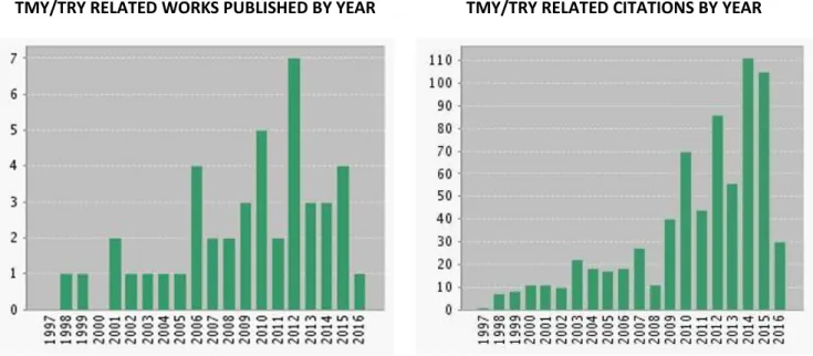
In Figure 1.1 the most relevant TMY/TRY research publications and the distribution through the years can be shown. 49 works has been selected from the Institute for Scientific Information (ISI) and using the Web of Science, citations of this selected works are shown. It is interesting to see how the industry needs pushed for an increasing number of works during 2012 which were cited and revised mainly during 2014 and 2015.
TMY/TRY RELATED WORKS PUBLISHED BY YEAR TMY/TRY RELATED CITATIONS BY YEAR
Figure 1.1. TMY/TRY related works and citation report since 1997.
For simulations of the thermal performance of buildings the ISO 15927-4 standard (ISO 15927-4, 2005) describes a standardized version of previous TRY methodologies: using dry-bulb tempera-ture, solar radiation and humidity as main variables; not specifying the weight of each variable but using a global ranking combination; using a two steps procedure based on the FS as the first step, but adding wind speed in a second step selection criterion among the three preselected through the ranking. This method is applied and well described in (Lee et al., 2010) and (Kalamees et al., 2012). In general, it is important to mention that the use of FS statistic is a very robust selection methodology because it does not rely on any specific probability distribution function to capture the internal variability of monthly or annual values.
Page 10 of 103
1.3 Recent works on the creation of reduced meteorological data sets
In recent years, the growing number of solar thermal electricity projects has pushed researchers to look for solutions to specific needs of this technology. Main topics to be discussed are related to: (1) the use of direct normal irradiance (DNI) as unique relevant input, or the need for additional related meteorological variables; (2) The use of measured and / or modeled data; (3) The need to provide probabilistic information for profitability assessments and annual payback.
There are works focused in typical solar radiation years (TSRY) (Mosalam Shaltout and Tadros, 1994; Zhou et al., 2006; Bulut, 2010; Zang et al., 2012) where relatively large weighting factors are given to the solar radiation variables compared to the TMY and TMY2 weighting factors. For solar thermal electricity (STE) applications, direct normal irradiance (DNI) is the single most important meteorological variable. Therefore, new methodologies where DNI is 100% weighted have been designed by Hoyer-Klick et al. (2009) or Habte et al. (2014). In addition to DNI a maximum wind threshold can be taken into account, as is shown in the ENDORSE TMY generation service (Espinar et al., 2012). In the case of the Spanish standard (AENOR, 2014), DNI can be weighted with 100% or with 50% sharing with global horizontal irradiance (GHI) the whole weight.
Threshold effective DNI as discussed by Rheinländer et al. (2008) and (Meyer et al., 2009), can re-place DNI to take into account the DNI angle of incidence, the shut down and the dumping effects respectively for too low and too high effective DNI, and the effect of wind speed above a certain speed threshold for which the collectors is in an security position.
Due to the high cost of solar radiation measurements and the impossibility to have 20 years of measurements in all locations with potential solar installations, the use of gridded data sets (Hoyer-Klick et al., 2009; Habte et al., 2014) has become essential. Gridded data sets cover all land points with a specific spatial resolution, unlike local measurements that provide information only for a specific location. Gridded data sets can be derived from satellite observation data, from nu-merical weather prediction (NWP) model analysis, or interpolated between ground-based meas-urement stations. In Zelenka et al. (1992) and Zelenka et al. (1999) validation exercises of several satellite-derived solar radiation databases are shown. They also analyzed the impact of distance from the nearest measurement station on the gridded data representation. Each of these options (satellite-derived data sets vs. measurements) has different qualities and uncertainties, which are not always clear to the user. In order to minimize uncertainties in the satellite data sets, at least one year of hourly ground-based measurements should be used for site-adaptation of the satellite data (Ramírez et al., 2012; Polo et al., 2015). This should be used to ensure that the satellite-derived data do not have major biases in daily profiles, even when monthly and yearly values could be similar. Site-adaptation can also provide empirical corrections for the effects of small scale clouds that the satellite images cannot resolve. Meyer et al. (2009) summarize requirements
Page 11 of 103
to satellite-derived irradiances, including the need for higher time resolution than one hour, site adaptation, and a minimum spatial resolution of 0.1°.
Although solar radiation is the main impact variable in STE power plants, in order to cover all the possible applications as well as to improve the system characterization, temperature, humidity and wind speed are also needed. For most meteorological variables the highest quality gridded data sets are obtained by re-analyzing all available and quality-controlled measurements with a numerical weather prediction (NWP) model (Daley, 1993). For solar irradiance data, this is, how-ever, not the case. Boilley and Wald (Boilley and Wald, 2015) show that both the ERA-Interim (Dee et al., 2011) and MERRA reanalysis (Rienecker et al., 2011) data sets are of lower quality than the best satellite-derived data sets. This may well change in the future as the NWP models used for reanalysis improve. Currently, reanalysis data sets are not recommended as a solar radiation data source.
In order to enable reliable profitability and annual pay back assessments, one annual series of meteorological data is not enough. Additional probabilistic information related to the energy out-put has to be available. Festa & Ratto started their work on statistical properties of solar radiation more than 20 years ago (Festa and Ratto, 1992); but this type of investigations where decoupled from the TMY assessments until 2013 (McMahan et al., 2013; Vignola et al., 2013), and in relation-ship with the fast growth of STE plants in Spain. A typical CSP project in Spain provides 50 MW nominal installed power. Such an installation could cost more than 300 M€ (Ruíz et al., 2011), and the investment of such size usually requires loans from banks. For risk analysis financial experts need to know the project’s incomes even in very bad years. For detailed analysis of potential cash flows they need information related to the probability distribution of the generated income through the years. It should be noted that this is not necessarily proportional to the probability distribution of the solar radiation through the years!
1.4 Ongoing initiatives and future needs
TMY Standardization is one of the main related ongoing initiatives, pushed and requested by
companies. Figure 1.2 shows timeline of TMY activities. When researchers are dealing with uncer-tainty, probability or variability topics, companies have needs related to harmonization of existing techniques In this context, the goal of this report is to focus on the future stakeholder needs for a standard approach to address the variability of solar and meteorological resources.
Page 12 of 103
Figure 1.2. TMY/TRY activities timeline. The researchers’ activities are a step ahead of the
standardization activities. The latter are mainly made on the initiative of companies even when researchers are also involved.
At the international level the IEC Technical Committee (TC) 117 Technical Specification (TS) 62862-1-2 is addressing the needs for solar resource and meteorological time-series data as input for simulating solar thermal electric (STE) systems. The main intention of this specification is to pro-vide a methodology for solar radiation yearly data set generation that propro-vides high-quality local series for solar thermal electricity projects. Typically, the TMY to be defined in IEC TS 62862-1-2 will be used for prefeasibility studies. The TS 62862-1-2 will include procedures for quality control, gap filling, combination of data sets from different sources, and replacement of daily data to get the monthly mean values. For financing of CSP/STE plants TMY data sets generated according to TS 62862-1-2 might be used as a base case. For detailed feasibility studies and profitability as-sessments of CSP/STE projects additional characterization of variability and uncertainty of the pro-vided TMY is needed.
The original draft is based on AENOR (2014), where one year of local surface measurements is re-quired, and at least of 10 years of gridded data, based on estimates from satellite observations, are strongly recommended (Figure 1.3) as a minimum requirement for preparation of sound
me-Page 13 of 103
teorological input data into performance simulation models. Two main options can be considered: the long-term gridded data adaptation to local measurements, the local measurements adaptation to the long-term gridded data. The first option is a simplification of the TMY or TRY, where local gridded data cover at least 10 years of DNI hourly values. These data have to be checked and cor-rected with the simultaneous hourly local measurements. In a second step, months are selected through calculation of FS based on DNI (and GHI if available). The long-term monthly value (LTMV) is derived from the selected month as the monthly sum. In addition to this option, the carefully revised local measurement can be used as the base for the TMY. Month by month, days of the local measurement are replaced by another near day trying to achieve the LTMV, calculated form the described methodology in the first option. As originally proposed by Hoyer-Klick et al. (2009) a maximum distance of 5 days between replaced days is allowed to prevent that sun angles and day length shows noticeable differences from the angles which should appear at the specific day, which is replaced. The now proposed IEC code further limits the maximum number of changes to 15 and the same day can only be used 4 times as an additional requirement to avoid to many iden-tical days.
Figure 1.3. Summary of the IEC standard for TMY generation. Two main options can be consid-ered:1. local measurements adaptation to the long-term gridded data; 2. long-term gridded data adaptation to local measurements. Where RMV re-fers to “Reference Monthly Value” and are the DNI or GHI monthly values in the final TMY, depending on the main variable for typical month selection considered in the approach. LT means “Long –Term”.
TMY data sets in general aim to express the most likely average weather situation at a site, which for CSP/STE plants is best characterized by the P50 DNI value expressing the 50% level of
exceed-Page 14 of 103
ance. In addition to the TMY standardization the financial community requests data sets for analy-sis of the DNI resource risk. Such meteorological data sets should either result in the electricity
generation in a very bad year and simultaneously the consequences of a systematic overestima-tion of DNI or only the latter effect. Typically, these data sets are designed in a way that the
aver-age DNI is representing a specific conservative case.
Various approaches for calculating such risk analysis data sets have been proposed in recent works (Cebecauer and Šúri, 2015; Roettinger et al., 2015). Proposals have a methodological path not so far from the TMY, using months as candidates among the worsts available months instead from the available mean months. Thus, the main differences are related to the way of selecting the bad months for building the low DNI year (Espinar et al., 2012; Fernández-Peruchena et al., 2015; Ce-becauer and Šúri, 2015).
The most requested annual series is that related to the 10th percentile of the DNI long-term aver-age in terms of statistical terminology. That is a meteorological year, which should be exceeded with a probability of 90 percent. Thus, such a case in energy finance usually is indicated b P90 – although statistics literature rather refers to such as P10.
When banks should finance CSP/STE-plants some ask for a P90-data sets representing only the more dramatic case, when the average DNI is overestimated due to uncertainty of the long-term mean DNI. As this P90-level is referring to the uncertainty of the multi-year average this is called
multi-year-P90. Other banks, which also want to see the effect of inter-annual variability in the
same data set, ask for a so called single-year-P90. Such P90single in addition to uncertainty consid-ers the effect of a year with unfavorable weather conditions for CSP-electricity production.
A debate related to adequate methodologies to generate this P90 series is still ongoing and will be discussed in future chapters. One discussion is related to the correlation between P90 meteoro-logical series vs. P90 energy output. The objective is to provide a P90 annual energy output, but there is not a linear correlation between an annual DNI value and an annual energy output. An-other open discussion is related to the possibility to build near infinite annual series with the same annual DNI value, and these series will derive into very different annual energy output values. In order to avoid the shortcomings of using single years there is the need to apply multi-year data sets. Pernigotto et al. (2014) show the influence of TRY data sets on the energy needs of buildings in five Italian locations. E.g., the energy output from a TRY month could be out of the
inter-quartile-range of all available monthly energy outputs for a specific month. Similar studies are now under evaluation for STE-projects and will have a importance in future years. The simplest multi-year data set is the use of gridded data sets locally corrected during the whole available period of years (typically more than 20), and use it to simulate the energy output (Fernández-Peruchena et al., 2015). The output data set gives sample years for possible annual electricity yields. From such
Page 15 of 103
results the frequency distribution due to natural variability of DNI can be fitted, which allows deri-vation of all percentiles. However, the approach of using multi-year data sets is only representing the resource risk due to inter-annual variability. The effect of a general systematic overestimation of the DNI due to uncertainty could be much severe and is not represented in multi-annual time-series, which on average should represent the P50 DNI.
To consider in addition to natural variability the effect of uncertainty on CSP/STE-yields Roettinger et al. (2015) make a first approach by manipulating DNI-values towards increased or reduced indi-vidual DNI values by simply multiplication with a linear factor. From application of such a wide population of synthetic years a frequency distribution of STE-yields can be derived, which is repre-senting both risk effects. Thus, from such a distribution function the single-year-P90 and other percentiles could be derived. This advanced statistical approach still needs to be verified and es-tablished in the energy and financial community.
1.5 Conclusions
For several decades yearly "Typical" and "Reference" meteorological data sets have been used for a broad range of solar technology simulations. Recently, specialized yearly data sets have been developed for specific solar technologies. Thus, users of yearly data sets need to use data sets de-signed for their purpose. A TMY that is weighted primarily with DNI is the current recommenda-tion for a yearly data set for CSP/STE simularecommenda-tions.
Standardization of procedures for TMY generation for STE projects has much progressed in the context of IEC TC 117. The respective Technical Specification is expected to be finished in 2016. It aims to define the most suitable methodology for generating an annual series of meteorological data for the simulation of solar thermal electricity power plants, which should represent the P50 long-term average of DNI. Such high quality and accuracy TMY data sets today should be used for obtaining the financial base cases, when financing a CSP/STE plant.
It is planned that IEC TC 117 in addition to a standardized TMY generation is preparing a code for generation of P90 or similar meteorological years. This code should clarify the most suitable methodology to obtain a data set from which the energy output of a bad cases could be calculat-ed. It should define how uncertainty of long-term DNI data should be calculated and how this leads to multi-year P90 levels. Further it should fix how the additional effect of natural variability has to be expressed in single-year P90 levels. With such a single-year P90 annual data set it can be evaluated how the debt-service is covered even if the very bad case of unfavorable CSP-weather occurs coincident with overestimation of DNI-averages. Very conservative risk assessments as-sume such in the first year of plant operation, when there are perhaps no reserve accounts filled.
Page 16 of 103
The approach of using only few annual data sets, such as a P50 TMY, and a P90 and perhaps a me-teorological year representing P75 DNI levels, has shortcomings: due to non-linear relation of DNI with power output of CSP/STE plants the resulting P90 level related to electricity production might significantly differ from the actual probability. Thus, methodologies that try to characterize the whole probability density function (PDF) of meteorological conditions through the power plant lifetime need to be investigated. Once the PDF of meteorological variables is clarified, an unlimited number of annual series can be synthesized.
1.6 References
AENOR, 2014. Centrales termosolares. Procedimiento de generación de Año Solar Representativo, UNE. UNE 206011.
Andersen, B., Eidorff, S., Lund, H., Pedersen, E., Rosenørn, S., Valbjørn, O., 1974. Referenceåret - Vejrdata for VVS beregninger, (The Reference Year - Weather data for HVAC-calculations), Report no. 89. Danish Building Research Institute.
Argiriou, A., Lykoudis, S., Kontoyiannidis, S., Balaras, C.A., Asimakopoulos, D., Petrakis, M., Kas-somenos, P., 1999. Comparison of methodologies for tmy generation using 20 years data for Athens, Greece. Solar Energy 66, 33–45.
doi:http://dx.doi.org/10.1016/S0038-092X(99)00012-2
Benseman, R.F., Cook, F.W., 1969. Solar radiation in New Zealand--The standard year. New Zea-land journal of science 12, 698–708.
Boilley, A., Wald, L., 2015. Comparison between meteorological re-analyses from ERA-Interim and MERRA and measurements of daily solar irradiation at surface. Renewable Energy 75, 135– 143. doi:10.1016/j.renene.2014.09.042
Bulut, H., 2010. Generation of representative solar radiation data for Aegean Region of Turkey. International Journal of the Physical Sciences 5, 1124–1131.
Cebecauer, T., Suri, M., 2015. Typical Meteorological Year Data: SolarGIS Approach. Energy Proce-dia 69, 1958–1969. doi:10.1016/j.egypro.2015.03.195
Daley, R., 1993. Atmospheric Data Analysis, Cambridge University Press. Cambridge University Press. Atmospheric and Space Science Series, New York, NY, USA.
Dee, D.P., Uppala, S.M., Simmons, A.J., Berrisford, P., Poli, P., Kobayashi, S., Andrae, U.,
Balmaseda, M.A., Balsamo, G., Bauer, P., Bechtold, P., Beljaars, A.C.M., van de Berg, L., Bidlot, J., Bormann, N., Delsol, C., Dragani, R., Fuentes, M., Geer, A.J., Haimberger, L., Healy, S.B., Hersbach, H., Hólm, E. V., Isaksen, L., Kållberg, P., Köhler, M., Matricardi, M., McNally, A.P., Monge-Sanz, B.M., Morcrette, J.-J., Park, B.-K., Peubey, C., de Rosnay, P., Tavolato, C.,
Page 17 of 103
the data assimilation system. Quarterly Journal of the Royal Meteorological Society 137, 553– 597. doi:10.1002/qj.828
Espinar, B., Blanc, P., Wald, L., 2012. Report on the production S4 “TMY FOR PRODUCTION,” in: Project ENDORSE. p. 12.
Fernández-Peruchena, C.M., Ramírez, L., Silva, M., Bermejo, D., Gastón, M., Moreno, S., Pulgar, J., Liria, J., Macías, S., Gonzalez, R., Bernardos, A., Castillo, N., Valenzuela, R.X., Zarzalejo, L., 2015. Estimation of the probability of exceedance of Direct Normal solar Irradiation series, in: Conference Proceedings SolarPACES. p. 5.
Festa, R., Ratto, C.F., 1993. Proposal of a numerical procedure to select Reference Years. Solar En-ergy 50, 9–17. doi:10.1016/0038-092X(93)90003-7
Festa, R., Ratto, C.F., 1992. Solar radiation statistical properties. Task 9, Solar Heating and Cooling. International Energy Agency.
Finkelstein, J.M., Schafer, R.E., 1971. Improved Goodness-Of-Fit Tests. Biometrika 58, 641. doi:10.2307/2334400
Habte, A., Lopez, A., Sengupta, M., Wilcox, S., 2014. Temporal and Spatial Comparison of Gridded TMY, TDY, and TGY Data sets, NREL/TP-5D00-60886. National Renewable Energy Laboratory. Hall, I.J.R., Prairie, R.R., Anderson, H.E., Boes, E.C., 1978. Generation of Typical Meteorological
Years for 26 SOLMET Stations, SAND78-1601. Sandia National Laboratories, Albuquerque, NM, USA.
Hoyer-Klick, C., Hustig, F., Schwandt, M., Meyer, R. (2009): Characteristic meteorological years from ground and satellite data. SolarPACES Symp., Berlin, Germany, Sep. 2009, 8 p.
ISO 15927-4, 2005. Hygrothermal performance of buildings -- Calculation and presentation of cli-matic data -- Part 4: Hourly data for assessing the annual energy use for heating and cooling. International Organization for Standardization, Geneva, Switzerland.
Kalamees, T., Jylhä, K., Tietäväinen, H., Jokisalo, J., Ilomets, S., Hyvönen, R., Saku, S., 2012. Devel-opment of weighting factors for climate variables for selecting the energy reference year ac-cording to the EN ISO 15927-4 standard. Energy and Buildings 47, 53–60.
doi:10.1016/j.enbuild.2011.11.031
Lee, K., Yoo, H., Levermore, G.J., 2010. Generation of typical weather data using the ISO Test Ref-erence Year (TRY) method for major cities of South Korea. Building and Environment 45, 956– 963. doi:10.1016/j.buildenv.2009.10.002
Lund, H., 1995. Design Reference Years. Task 9, Solar Heating and Cooling. International Energy Agency.
Page 18 of 103
published as: Report no. 32, Thermal Insulation Laboratory, Technical University of Denmark, in: Second Symposium on the Use of Computers for Environmental Engineering Related to Building. Paris (France), p. 12.
Marion, W., Urban, K., 1995. User’s Manual for TMY2s, NREL. National Renewable Energy Labora-tory, Golden.
McMahan, A.C., Grover, C.N., Vignola, F.E., 2013. Evaluation of Resource Risk in Solar-Project Fi-nancing, in: Solar Energy Forecasting and Resource Assessment. Elsevier, pp. 81–95. doi:10.1016/B978-0-12-397177-7.00004-8
Meyer, R., Beyer, H.G., Fanslau, J., Geuder, N., Hammer, A., Hirsch, T., Hoyer-klick, C., Schmidt, N., Schwandt, M., 2009. Towards Standardization Of CSP Yield Assessments, in: Proceedings of the SolarPACES Conference. Berlin, p. 8.
Mosalam Shaltout, M.A., Tadros, M.T.Y., 1994. Typical solar radiation year for Egypt. Renewable Energy 4, 387–393. doi:10.1016/0960-1481(94)90045-0
Pernigotto, G., Prada, A., Cóstola, D., Gasparella, A., Hensen, J.L.M., 2014. Multi-year and refer-ence year weather data for building energy labelling in north Italy climates. Energy and Build-ings 72, 62–72. doi:10.1016/j.enbuild.2013.12.012
Petrakis, M., Kambezidis, H.D., Lykoudis, S., Adamopoulos, A.D., Kassomenos, P., Michaelides, I.M., Kalogirou, S.A., Roditis, G., Chrysis, I., Hadjigianni, A., 1998. Generation of a “typical meteoro-logical year” for Nicosia, Cyprus. Renewable Energy 13, 381–388.
doi:10.1016/S0960-1481(98)00014-7
Petrie, W.R., McClintock, M., 1978. Determining typical weather for use in solar energy simula-tions. Solar Energy 21, 55–59. doi:10.1016/0038-092X(78)90116-0
Pissimanis, D., Karras, G., Notaridou, V., Gavra, K., 1988. The generation of a “typical meteorologi-cal year” for the city of Athens. Solar Energy 40, 405–411. doi:10.1016/0038-092X(88)90095-3.
Polo, J., S. Wilbert, J. A. Ruiz-Arias, R. Meyer, C. Gueymard, M. Šúri, L. Martín, T. Mieslinger, P. Blanc, I. Grant, J. Boland, P. Ineichen, J. Remund, R. Escobar, A. Troccoli, M. Sengupta, K. P. Nielsen, D. Renne, N. Geuder, 2015. Integration of ground measurements to model-derived data. IEA Report from SHC Task 46: Solar Resource Assessment and Forecasting.
Ramírez, L., Barnechea, B., Bernardos, A., Bolinaga, B., Cony, M., Moreno, S., Orive, R., Polo, J., Redondo, C., Salbidegoitia, I.B., Serrano, L., Tovar, J., Zarzalejo, L.F., 2012. Towards the stand-ardization of procedures for solar radiation data series generation, in: Proceedings of the So-larPACES Conference. p. 5.
Rheinländer, J., Bergmann, S., Erbes, M. R., 2008. Technical and economic performance of parabol-ic trough solar power plants—A computational tool for plant feasibility studies. In 14th So-larPACES International Symposium on Concentrated Solar Power and Chemical Energy
Tech-Page 19 of 103
nologies, Las Vegas, NV, USA.
Rienecker, M.M., Suarez, M.J., Gelaro, R., Todling, R., Bacmeister, J., Liu, E., Bosilovich, M.G., Schu-bert, S.D., Takacs, L., Kim, G.-K., Bloom, S., Chen, J., Collins, D., Conaty, A., da Silva, A., Gu, W., Joiner, J., Koster, R.D., Lucchesi, R., Molod, A., Owens, T., Pawson, S., Pegion, P., Redder, C.R., Reichle, R., Robertson, F.R., Ruddick, A.G., Sienkiewicz, M., Woollen, J., 2011. MERRA: NASA’s Modern-Era Retrospective Analysis for Research and Applications. Journal of Climate 24, 3624–3648. doi:10.1175/JCLI-D-11-00015.1
Ruíz, V., Blanco, M., Maraver, A., Silva, M., Ramírez, L., Cárdenas, B., Lillo, I., Sánchez, M., Regidor, A., Moreno, S., García-Barberena, J., Muñóz, J., Domínguez, J., Gracía, P., Pallardo, I., Pascal, E., Luna, S., 2011. Evaluación del potencial de energía solar termoeléctrica: Estudio tecnico PER 2011 - 2020, IDAE. IDAE.
Röttinger, N., Remann, F., Meyer, R., Telsnig, T., 2015. Calculation of CSP yields with probabilistic meteorological data sets: a case study in Brazil. Energy Procedia, 69, 2009-2018.
Stoffel, T., 1998. Production of the Weather Year for Energy Calculations Version 2 (WYEC2). NREL TP-463-20819. National Renewable Energy Laboratory, Golden, CO, USA.
Varela, M., Ramírez, L., Mora, L., Sidrach de Cardona, M., 2004. Economic analysis of small photo-voltaic facilities and their regional differences. International Journal of Energy Research 28, 245–255. doi:10.1002/er.963
Vignola, F.E., McMahan, A.C., Grover, C.N., 2013. Bankable Solar-Radiation Data sets, in: Solar En-ergy Forecasting and Resource Assessment. Elsevier, pp. 97–131. doi:10.1016/B978-0-12-397177-7.00005-X
Wilcox, S., Marion, W., 2008. User's Manual for TMY3 Data sets, NREL/TP-581-43156. National Renewable Energy Laboratory.
WMO, 2011. Guide to climatological practices, WMO. World Meteorological Organization, Geneva. Zang, H., Xu, Q., Bian, H., 2012. Generation of typical solar radiation data for different climates of
China. Energy 38, 236–248. doi:10.1016/j.energy.2011.12.008
Zelenka, A., Czeplak, G., D’Agostino, V., Josefsson, W., Maxwell, E., Perez, R., 1992. Techniques for supplementing solar radiation network data. Volume 1. Task 9, Solar Heating and Cooling. In-ternational Energy Agency.
Zelenka, A., Perez, R., Seals, R., Renné, D., 1999. Effective Accuracy of Satellite-Derived Hourly Ir-radiances. Theoretical and Applied Climatology 62, 199–207. doi:10.1007/s007040050084 Zhou, J., Wu, Y., Yan, G., 2006. Generation of typical solar radiation year for China. Renewable
Page 20 of 103
2.
Uncertainty of DNI values
All data, whether measured or modeled, is uncertain. The uncertainty is important to quantify and account for in simulations and statistical analyses. Uncertainty should not be confused with the actual variability of the data. Here the uncertainties in vari-ous sources of DNI data are described and discussed.
The performance of a solar thermal electric (STE) facility is linearly dependent upon the Direct Normal Irradiance (DNI), the solar flux coming directly from the disk of the sun and the area im-mediately adjacent to the solar disk. Any uncertainty in the DNI leads to equivalent uncertainty in the estimated STE facility performance. There are two main sources of DNI resource information. One is measured with ground-based instruments and the other derived from models that utilize information from satellites. There are a wide variety of methods that utilize information from sat-ellites and other sources to estimate the DNI resource. These methods range from models that use reanalysis data in which satellite and other measurements are combined with atmospheric models to estimate DNI (Daley, 1993) to more empirical models that rely on correlations of cloud cover data from satellite images and measured irradiance.
As with all measurements, the solar irradiance measurements are not exact and there are uncer-tainties associated with obtaining the DNI values. Before going into an analysis of the uncertain-ties associated with obtaining DNI values from ground-based measurements or from modeling satellite data, the characteristics and nature of uncertainties are discussed. The discussion on un-certainties will be followed by a detailed description of the unun-certainties associated with ground-based and satellite-derived DNI values. The use of ground-ground-based measurements to validate and/or adjust satellite-derived values is then examined. Characterization of differences between ground-based measurements and satellite-derived values can be used to reduce uncertainties and better quantify biases in satellite-derived DNI values.
2.1 Uncertainty in Measurements
All measurements have an uncertainty associated with the measurement. These uncertainties are dependent on the instruments used, the way the measurements are made, and the manner in which the measurements are recorded. For example, when one measures the length of a table a number of times, the results will likely vary slightly. If the same measurement is made by another person, the results will vary from the first observations because the tape measure may be read slightly differently or the perceived edge of the table may differ. If one uses a different tape measure, one could get a slightly different set of measurements because the tape measures may not match exactly. Other factors such as temperature may affect the measurement because the expansion rate of the tape measure will likely differ from that of the table.
Page 21 of 103
In general, length can be measured with great accuracy, especially if lasers are used because the wavelength of light is used to define the standard meter and the wavelength of laser light can be measured to a very high degree of accuracy. Even these reference measurements have some as-sociated degree of uncertainty as required by the fundamental Heisenberg uncertainty principle. The act of repeated measurements of any object will generate a set of values and in most cases, these values are randomly distributed and the set of data will form a Gaussian distribution around some average value. Conditions for data following the Gaussian distribution are given by the cen-tral limit theorem. The average or mean value is the sum of the measurement values divided by the number of measurements. The half-width of the Gaussian distribution is defined as one standard deviation and about 68% of the data points will be less than one standard deviation from the average value. Standard deviation is a measure of the spread of measurement values. It is the square root of the average of the squared differences from the mean. Approximately 95% of the measured values will fall within two standard deviations of the mean. Therefore one can charac-terize the probability that a measurement is within a given percentage of the mean value by exam-ining the distribution of the measurements about the mean. This type of uncertainty is referred to as random uncertainty and helps define the likelihood that the measurement will be within a given uncertainty of the exact value.
Another type of uncertainty is exhibited by two different measuring devices. Consider the tape measure example. One tape measure might have a slightly different length scale than the other tape measure. The two different tape measures will then exhibit a bias compared to the other tape measure depending on the amount of the difference in the scale or markings on the two tape measures. The length from one tape measure will produce a longer or shorter mean distance as compared with the other tape measure. Part of this uncertainty is related to the precision on the distance markers on the tape measure and the other relates accuracy to which the tape measure can be read. These uncertainties are usually assigned to the tape measure and are not measured against a standard. Therefore the manufacturer will say that the uncertainty of the tape measure is ±2 mm and that information can be used when combining all the uncertainties.
To standardize the discussion of uncertainties and to set standards that provide guidelines for de-termining uncertainty and characterizing uncertainties, the Guide to Expressing Uncertainties in
Measurements (GUM) was created (ISO, 2008). This document explains in detail the GUM
termi-nology and explains how to perform uncertainty analysis using the GUM procedures. Several pa-pers are now available evaluating irradiance measurements using the GUM methodology and the uncertainties discussed in this document are based on the GUM terminology (JCGM/WG 1, 2008). The GUM model starts by defining the “measurand”, the quality that is being measured. The re-sulting measurement is an approximation or estimate of the measurand and a full description of the measurement includes the uncertainty of the measurement. In addition, other environment quantities that affect the measurement should be included. For example, the WRR calibrations are measurements of DNI made when DNI values >700 W/m2 under clear sky, stable weather condi-tions. Measurements are not exact and there are uncertainties in the measurements. Traditional-ly, errors are viewed as having two components, a random and a systematic component.
Page 22 of 103
Random errors arrive from unpredicatable or stochastic temporal and spatial variations of quanti-ties that influence the measurements. These variations are called random effects and result in the variations of repeated measurements of the measurand. Random errors can usually be reduced by increasing the number of measurements. The experimental standard deviation is a measure of the uncertainty of the mean resulting from random effects.
Systematic errors arise from a recognized effect that influences the measurements. The effect can be quantified and if it is significant in size, a correction factor can be devised and applied to com-pensate for the effect. The uncertainty in the correction factor is a measure of incomplete knowledge of the value required for the correction. The terms error and uncertainty should be used precisely and care should be taken to distinguish them.
The following is a sampling of possible sources of uncertainty in measurements from the GUM document.
a) Incomplete definition of the measurand;
b) Imperfect reaIization of the definition of the measurand;
c) Nonrepresentative sampling — the sample measured may not represent the defined measurand;
d) Inadequate knowledge of the effects of environmental conditions on the measurement or imperfect;
e) Measurement of environmental conditions; f) Personal bias in reading analogue instruments;
g) Finite instrument resolution or discrimination threshold;
h) Inexact values of measurement standards and reference materials;
i) Inexact values of constants and other parameters obtained from external sources and used in the data-reduction algorithm;
j) Approximations and assumptions incorporated in the measurement method and proce-dure;
k) Variations in repeated observations of the measurand under apparently identical condi-tions.
The sources of uncertainty are not necessarily independent. In addition, unrecognized systematic effects can contribute to the error in the measurement.
The GUM methodology breaks the uncertainties into two Types, A and B. Both types are quanti-fied by variances and/or standard deviations.
The Type A evaluation is calculated from series of repeated observations and is the familiar statis-tically estimated variance. The estimated standard deviation for Type A evaluations is sometimes called Type A standard uncertainty.
For the Type B evaluations, the variance is evaluated using available knowledge, for example the characteristics of the measuring device. This estimated standard deviation is sometimes called a
Page 23 of 103
Type B standard deviation. For example, if the specifications for the pyrheliometer state that it has a temperature dependence of ±0.5%, then Type B standard deviation is ±0.5%.
The GUM methodology then adds the uncertainties by quadrature (this approach has to be modi-fied if the uncertainties are covariant). Adding in quadrature is summing the square the numbers and taking the square root of the sum. An expanded uncertainty is then generated by a coverage factor to give the level of confidence that the measurement accurately represents the measurand. For example for a 95% confidence level, the coverage factor is approximate 2 (1.96). Given an expanded uncertainty with a 95% confidence level is equivalent to saying that 95% of the meas-urements will be within the expanded uncertainty of the measurand.
Before going into a more detailed description of measurement uncertainties, the effects of time scales on uncertainties should be mentioned. All irradiance data are for a given time period whether it is instantaneous or hourly, daily, or monthly average values. As the time scale increas-es, the uncertainty decreases because random uncertainties tend to average out and some bias uncertainties may be offset by other bias uncertainties with opposite effects. For example, many pyrheliometers that measure DNI have a responsivity (i.e. microvolts per W/m2) that varies in a systematic manner over the day. The calibration used for the pyrheliometer to change the voltage reading into irradiance is commonly determined when the solar zenith angle is 45. (The calibra-tion value for a pyrheliometer is 1 divided by the responsivity.) When the sun is higher in the sky the responsivity might be slightly higher than when the sun in lower in the sky. Therefore, the uncertainty in the measurement will vary slightly over the day. If one takes the daily average, the daily uncertainty will be less because the overestimate may be when the sun is higher in the sky is offset by the underestimate when the sun is lower in the sky. This means that when one is talking about hourly uncertainties, the uncertainty will likely be greater than when one is talking about daily or monthly average uncertainties. Therefore, it is important to specify the time scale when giving an uncertainty of the measurements.
2.2 Ground-based DNI value uncertainties
Ground-based DNI measurements can be recorded virtually instantaneous or averaged over time periods from one-minute to daily. The most accurate DNI measurements are made with electri-cally self-calibrating absolute cavity radiometers (ACR) that compare the thermal heating of the DNI against a known electrical power used to heat the detector to the same temperature as the DNI. The ACR DNI measurements are used as reference values because electrical current can be measured to a much higher degree of accuracy than measurements of thermal energy. The inter-nationally recognized standard for DNI is the World Radiometric Reference (WRR) developed and maintained by the World Radiation Center (WMO 2011). The WRR is a detector-based measure-ment reference defined by six radiometers comprising the World Standard Group (WSG). The WRR is known to ± 0.3% at the 99% level of confidence for DNI greater than 700 W/m2 (WMO, 2011, Frohlich, 1978). This accuracy is achieved under stable clear-sky conditions. Periodically,
Page 24 of 103
other ACRs are calibrated against this standard and they achieve accuracies, at the 95% level of confidence, in the range of ±0.36% to 0.40% (Reda, 2014). These calibrated ACRs and then used to calibrate other DNI measuring instruments. All certifiable calibrations of DNI measuring instru-ments can trace their calibrations to the WRR.
ACR’s are very expensive and are not intended for field operation. Many ACRs do not provide a continuous time series and are not designed to work under unstable weather conditions. Few long-term data sets using ACRs are available. ACRs with the lowest uncertainties have an aperture open to the atmosphere. This allows moisture, dust, and insects to enter the device. Some ACRs come equipped with windows that allow the use of the instrument under all weather conditions. Alternatively one can build a shelter that closes at night or under conditions, such as rain, that would damage the instrument (Vuilleumier, 2014). ACRs with windows are said to have an uncer-tainty of ±0.5% (McArthur, 2005). These uncertainties are for instantaneous measurements and not averaged over time. All uncertainties mentioned in this section have are at the 95% level of confidence unless otherwise noted.
Besides the ACR instruments, there are four ways to obtain DNI values from ground-based meas-urements:
1. Field Pyrheliometers
2. Rotating Shadowband Irradiometers 3. Pyranometers with a shadow masks
4. Calculations using Global Horizontal Irradiance (GHI) and Diffuse Horizontal Irradiance (DfHI)
In most cases there are many varieties of each type of DNI instrument. This chapter is a general overview and only specific information will be given for a limited number of instruments.
2.2.1 Pyrheliometers
Most field pyrheliometers consist of thermopiles-based detectors at the end of a collimation tube that has a window covering the aperture. Voltage generated by the thermopile inside the pyrheli-ometer is proportional to the incident solar irradiance. The aperture and the collimation tube provide an opening with a full angle of view between 5.0 and 5.7. The size of the opening angle was determined help ensure that solar tracker pointing inaccuracies did not significantly affect the measurements (CIMO, 2008). Newer models of pyrheliometers have 5.0 field of view that
matches the geometry of ACRs. Along with the light coming directly from the sun, some circumso-lar irradiance is added to the DNI irradiance value. Many concentrating technologies cannot utilize the circumsolar irradiance and this has to be considered when employing measured DNI values for STE performance estimates (Blanc et al., 2014). The preferred calibration of a pyrheliometer is against an ACR that has calibration traceability to the World Radiometric Reference (WRR). In the
Page 25 of 103
field a pyrheliometer can also be calibrated against another pyrheliometer that has its calibration traceable to the WRR. This method will result in a slightly larger estimated measurement uncer-tainty.
Thermopile-based instruments have a time constant associated with the time it takes for the in-strument to reach thermal equilibrium. This time constant can vary from a few seconds to tens of seconds, depending on the thermal characteristics of the pyrheliometer. Clouds moving in front of the sun can drop the DNI very quickly. The pyrheliometer’s response time can affect average DNI measurements for time spans of less than a minute or when comparing DNI values with DNI values obtain from photodiode based devices that have response times on the order of seconds. Cali-brations of thermopile pyrheliometers are best performed with stable sky conditions (conditions that do not change rapidly).
The sources and types of uncertainty for DNI measured by pyrheliometers are given in Table 2.1. Good record keeping enables one to keep track of the maintenance and calibration history of the
Source Orgin of Uncertainty Type of Uncertainty Corrections Exist
Light source Uncertainty in Type B No
reference measurements
Instrument
Calibration Type A and B No
Non-linearity of response Type A and B No
Time of day Type A No
Detector stability Type A Yes
Temperature effects Type A or B Exists for some instruments
Maintenance Soiling Type B No
Moisture on window Type B No
Tracker Alignment Type B No
Measurement Data logger Type B No
Table 2.1: Source of Uncertainty for Pyrheliometers. The A and B type of uncertainties are described in section 2.1.
Page 26 of 103
instrument and any problems that occur while data is being gathered. Records should also include a site diagram to identify and characterize any obstruction affects the recorded DNI. Good loca-tions have obstrucloca-tions that are no more than 5 above the horizon.
For instantaneous measurements, the uncertainties for DNI measurements can be as low as 0.75% to 1.5%, but the uncertainty of even well maintained stations is estimated to be ±2.5% (Stoffel et al., 2010) as a result of many minor potential sources of uncertainty. Of course when instruments are not maintained or records of calibrations are absent, the uncertainty in the data can be much larger.
2.2.2 Rotating Shadowband Irradiometers
Rotating Shadowband Irradiometers (RSI) are instruments with one pyranometer measuring global horizontal irradiance (GHI) and diffuse horizontal irradiance (DfHI) as a band (shadowband) that rotates in above the pyranometer to block the direct sunlight. Rotation periods are typically one-minute or shorter. When the sun is blocked, the DfHI is measured. The direct horizontal irradiance (DrHI) is then obtained by subtracting the DfHI from the GHI (Eq. 2.1). The DNI value is then calcu-lated by dividing the DrHI by the cosine of the incident solar zenith angle (Eq. 2.2).
DrHI = (GHI – DfHI) (2.1) DNI = DrHI/cos(SZA) (2.2) where SZA is the solar zenith angle. When instantaneous measurements are used, this formula is exact. When the measurements of GHI and DfHI (or equivalently DrHI) are integrated over time, then the equation becomes an approximation because the SZA has to be averaged over the same time period and the average value of cos(SZA) is weighted by the changing DrHI (Vignola and McDaniels, 1986).
There are two types of RSI. One type uses fast photodiode based pyranometers to measure the GHI and the shadowband swipes across the sensor in a continuous motion. Extensive evaluations have been made on this type of RSI (Stoffel et al., 2010; Wilbert et al., 2015a; Sengupta et al., 2016; Vuilleumier et al., 2014; Vignola, 2006). Another type, the Total Solar Radiometer (TST), has the shadowband that stops its rotation in three places during the sweep. The first is just before it shades the pyranometer, the second is when it is shading the pyranometer, and the third is when it has just finished shading the pyranometer. During the stops it is possible to calculate the por-tion of the DfHI shaded of the shadowband. For RSI instruments with continuous rotations, the extra shading of the band is estimated during rotation. The slow speed and stopping of the shad-owband allows a thermopile-based pyranometer with a quick response time to be used for meas-uring the irradiance. Because the shadowband stops while shading the pyranometer, a thermopile based pyranometer can be used. A recent study of radiometers (Habte et al., 2016) at NREL con-tains an example of a TST instrument.
Page 27 of 103
The most common RSI being deployed are the instruments using photodiode-based pyranometers. The problem with photodiode-based pyranometers is that their output is dependent on the spec-tral distribution of the incident solar radiation. Of even more concern is that the responsivity of the pyranometer to the DNI spectral irradiance is different than the responsivity of the pyranome-ter to DfHI spectral irradiance on clear and partially clear days. There have been several studies to characterize this spectral dependence and algorithms (Vignola, 2006; King et al., 1997; Wilbert et al., 2015a; Vignola et al., 2015) have been developed to account for the differences in the DNI and DfHI spectral irradiances. Models have also been developed to account for the uncertainty effects of temperature and deviations from true cosine response.
Photodiode-based pyranometers do not fit specifications of the WMO for first-class instrument performance because of the dependence on the spectral distribution of the incident irradiance. They are widely used because they are relatively inexpensive and can produce results that are equivalent to second class pyranometer producing GHI values with uncertainties within ±5%. Pho-todiode-based pyranometers are used in RSI instruments because they have a quick response time on the order of seconds. Algorithms have been developed to account for much of the spectral dependence and other shortcomings of the photodiode-based pyranometer.
Because of the similarity between the photodiode and the solar cell, some postulate that these pyranometers produce results that more directly mimic photovoltaic module output than thermo-pile-based pyranometers. This assertion has not been satisfactorily validated by peer reviewed articles. That said, algorithms have been developed that mimic the spectral and cosine response of the photodiode pyranometer and account for the thermal dependence of the instrument. Often RSI instruments have been installed in remote locations or locations where the instruments are not maintained on a daily basis because acrylic diffusers can be more dust tolerant that optical glass domes or windows used by thermopile-based pyranometers to protect the detector. In the report of Maxwell et al. (1999) a list of papers that have studied this can be found. While the pyr-heliometers on both manually adjusted and automatic solar trackers potentially have less uncer-tainty in the reported results when they are well maintained, they are more sensitive to the buildup of dust on the window resulting in scattering and absorption of DNI as it enters the pyrhe-liometer. Lack of maintenance allows the buildup of dust on the window that increases the uncer-tainty of the measurements and this can significantly reduce the measured DNI if the dust is not removed on a regular basis.
Page 28 of 103
In RSI instruments, algorithms also account for the spectral differences between the DNI and DfHI responsivities. Using these algorithms, DNI values produced using RSIs have been shown to have uncertainties of less than ±3.5% (Vignola, 2012). A list of factors involved in the uncertainties as-sociated with RSI is shown in Table 2.2. The main concern about the adjustment algorithms is whether they apply as well in areas with atmospheric conditions that deviate significantly from the atmospheric conditions at the site(s) used to derive the adjustment algorithms. Specifically, this is the spectral or air mass adjustment. It has been shown that the spectral distribution on incident irradiance changes over the day in a systematic manner and that this affects the responsivity (and the output) of the photodiode based pyranometer. The change can be modeled as a function of air mass and this air mass adjustment is incorporated into the RSI adjustments (Vignola, 2006; King et al., 1997; Wilbert et al. 2015b; Vignola et al., 2015). Research is continuing to evaluate,
vali-date, and possibly improve the algorithms used to adjust the RSI’s GHI, DNI, and DfHI values. 2.2.3 Pyranometers with Shadow Mask
Pyanometers with a shadow mask is a multi-sensor pyranometer that measures GHI and DfHI and calculates DrHI and hence DNI from the difference between the GHI and DfHI measurements (see Eq. 2.1 and Eq. 2.2). The instrument that is currently available has seven small thermopiles dis-tributed on the base of the instrument under a specially designed shield that shades half the sky and always permits at least one of the sensors to be totally unshaded and one sensor to be totally shaded. Since the shield obscures half the sky dome, the value obtained from the pyranometer that is totally shaded is doubled to estimate the DfHI value.
Source Orgin of Uncertainty Type of Uncertainty Corrections Exist
Light source Uncertainty in refrence
measurements Type B No
Instrument
Spectral sensitivity Type A and B Yes
Calibration Type A and B No
Deviation from true
co-sine response Type A Yes Temperature effects Type A or B Yes
Detector stability Type A Yes
Non-linearity in
re-sponse Type B No
Maintenance
Soiling Type B No
Moisture on diffuser Type B No
Leveling Type B No
Measurement Data loggers Type B No