HAL Id: hal-00862230
https://hal.inria.fr/hal-00862230v2
Preprint submitted on 16 Sep 2013
HAL is a multi-disciplinary open access
archive for the deposit and dissemination of
sci-entific research documents, whether they are
pub-lished or not. The documents may come from
teaching and research institutions in France or
L’archive ouverte pluridisciplinaire HAL, est
destinée au dépôt et à la diffusion de documents
scientifiques de niveau recherche, publiés ou non,
émanant des établissements d’enseignement et de
recherche français ou étrangers, des laboratoires
Generalized Symmetry Breaking Tasks
Armando Castañeda, Damien Imbs, Sergio Rajsbaum, Michel Raynal
To cite this version:
Armando Castañeda, Damien Imbs, Sergio Rajsbaum, Michel Raynal. Generalized Symmetry
Break-ing Tasks. 2013. �hal-00862230v2�
Publications Internes de l’IRISA ISSN : 2102-6327
PI 2007 – September 2013
Generalized Symmetry Breaking Tasks
Armando Castañeda* Damien Imbs** Sergio Rajsbaum*** Michel Raynal****
Abstract: Processes in a concurrent system need to coordinate using an underlying shared memory or a message-passing system in order to solve agreement tasks such as, for example, consensus or set agreement. However, coor-dination is often needed to break the symmetry of processes that are initially in the same state, for example, to get exclusive access to a shared resource, to get distinct names, or to elect a leader.
This paper introduces and studies the family of generalized symmetry breaking (GSB) tasks, that includes election, renaming and many other symmetry breaking tasks. Differently from agreement tasks, a GSB task is inputless, in the sense that processes do not propose values; the task only specifies the symmetry breaking requirement, independently of the system initial state (where processes differ only on their identifiers). Among various results characterizing the family of GSB tasks, it is shown that perfect renaming is universal for all GSB tasks.
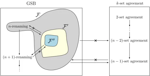
The paper then studies the power of renaming with respect tok-set agreement. It shows that, in a system of n processes, perfect renaming is strictly stronger than(n−1)-set agreement, but not stronger than (n−2)-set agreement. Furthermore,(n + 1) renaming cannot solve even (n − 1)-set agreement. As a consequence, there are cases where set agreement and renaming are incomparable when looking at their power to implement each other.
Finally, the paper shows that there is a large family of GSB tasks that are more powerful than(n−1)-set agreement. Some of these tasks are equivalent ton-renaming, while others lie strictly between n-renaming and (n + 1)-renaming. Moreover, none of these GSB tasks can solve(n − 2)-set agreement. Hence, the GSB tasks have a rich structure and are interesting in their own. The proofs of these results are based on combinatorial topology techniques and new ideas about different notions of non-determinism that can be associated with shared objects. Interestingly, this paper sheds a new light on the relations linking set agreement and symmetry breaking.
Key-words: Agreement, Asynchronous read/write model, Coordination, Concurrent object, Crash failure, Decision task, Distributed computability, Non-determinism, Problem hierarchy, Renaming, Set agreement, Symmetry breaking, Wait-freedom.
L’univers des tâches réparties de cassage généralisé de la symmétrie
Résumé : Ce rapport présente une étude exhaustive sur les tâches dont le but est de casser de la symmétrie dans un système réparti.
Mots clés : Accord réparti, Asynchronisme, Cassage de la symmétrie, tâche répartie.
*Department of Computer Science, Technion, Haifa, Israel **Instituto de Matematicas, UNAM, Mexico
***Instituto de Matematicas, UNAM, Mexico
1
Introduction
1Processes of a distributed system coordinate through a communication medium (shared memory or message-passing subsystem) to solve problems. If no coordination is ever needed in the computation, we then have a set of centralized, independent programs rather than a global distributed computation. Agreement coordination is one of the main issues of distributed computing. As an example, consensus [30] is a very strong form of agreement where processes have to agree on the input of some process. It is a fundamental problem, and the cornerstone when one has to implement a replicated state machine (e.g.,[26, 48, 53]).
We are interested here in coordination problems modeled as tasks [44, 52]. A task is defined by an input/output relation∆, where processes start with private input values forming an input vector I and, after communication, indi-vidually decide on output values forming an output vectorO, such that O ∈ ∆(I). Several specific agreement tasks have been studied in detail, such as consensus and set agreement [24]. Indeed, the importance of agreement is such that it has been studied deeply, from a more general perspective, defining families of agreement tasks, such as loop
agreement [43], approximate agreement [28] and convergence [42].
Motivation While the theory of agreement tasks is pretty well developed e.g. [40], the same substantial research effort has not yet been devoted to understanding coordination problems where “break symmetry” among the processes that are initially in a similar state is needed. Only specific forms of symmetry breaking have been studied, most notably mutual exclusion [27] and renaming [7]. It is easy to come up with more natural situations related to symmetry breaking. As a simple example, considern persons (processes) such that each one is required to participate in exactly one ofm distinct committees (process groups). Each committee has predefined lower and upper bounds on the number of its members. The goal is to design a distributed algorithm that allows these persons to choose their committees in spite of asynchrony and failures.
Similarly, some attention has been devoted in the past to understanding the relative power of agreement and sym-metry breaking tasks, but very little is known. There are only two results [31, 36] that measure the relative power of renaming and set agreement; even more, these result focus in very specific instances of these families of tasks. In-deed, [36] is the first that compares the computability power of renaming and set agreement: it shows that(n − 1)-set agreement (ink-set agreement, processes agree on at most k input values) is strictly stronger than (2n − 2)-renaming, namely,(n − 1)-set agreement solves (2n − 2)-renaming but not vice versa. Then, [31] showed that k-set agreement solves(n + k − 1)-renaming. Certainly, [31] considers the adaptive version of (n + k − 1)-renaming, however, clearly the result has implications for the non-adaptive version.
The aim of this paper is to develop the understanding of symmetry breaking tasks and their relation with agreement tasks, motivated by [36].
Generalized symmetry breaking tasks In this paper we introduce generalized symmetry breaking (GSB), a family of tasks that includes election, renaming, weak symmetry breaking [36, 44]2, and many other symmetry breaking tasks. A GSB task forn processes is defined by a set of possible output values, and for each value v, a lower bound and an upper bound (resp.,ℓv anduv) on the number of processes that have to decide this value. When these bounds vary
from value to value, we say it is an asymmetric GSB task. For example, we can define the election asymmetric GSB task by requiring that exactly one process outputs1 and exactly n − 1 processes output 2 (in this form of election, processes are not required to know which process is the leader).
In the symmetric case, we use the notationhn, m, ℓ, ui-GSB to denote the task on n processes, for m possible output values, where each value has to be decided at leastℓ and at most u times. In the m-renaming task, the processes have to decide new distinct names in the set[1..m]. Thus, m-renaming is nothing else than the hn, m, 0, 1i-GSB task. In thek-weak symmetry breaking task a process has to decide one of two possible values, and each value is decided by at leastk and at most (n − k) processes. This is the hn, 2, k, n − ki-GSB task. Let us notice that 1-WSB is the weak symmetry breaking task.
1Preliminary versions of the results presented in this report appeared in the proceedings of the 18th International Colloquium on Structural
Infor-mation and Communication Complexity (SIROCCO 2011) [45], the proceedings of the 10th Latin American Theoretical INformatics Symposium (LATIN 2012) [23], and the proceedings of the 27th IEEE International Symposium on Parallel and Distributed Processing (IPDPS’13) [22].
Symmetry breaking tasks seem more difficult to study than agreement tasks, because in a symmetry breaking task we need to find a solution given an initial situation that looks essentially the same to all processes. For example, lower bound proofs (and algorithms) for renaming are substantially more complex than for set agreement (e.g., [18, 44]). At the same time, if processes are completely identical, it has been known for a long time that symmetry breaking is impossible [6] (even in failure-free models). Thus, as in previous papers, we assume that processes can be identified by initial names, which are taken from some large space of possible identities (but otherwise they are initially identical). In an algorithm that solves a GSB task, the outputs of the processes can depend only on their initial identities and on the interleaving of the execution.
The symmetry of the initial state of a system fundamentally differentiates GSB tasks from agreement tasks. Namely, the specification of a symmetry breaking task is given simply by a set of legal output vectors denotedO that the processes can produce: in any execution, any of these output vectors can be produced for any input vectorI (we stress that an input vector only defines the identities of the processes), i.e.,∀I we have ∆(I) = O. For example, for the election GSB task,O consists of all binary output vectors with exactly one entry equal to 1 and n − 1 equal to 2. In contrast, an agreement task typically needs to relate inputs and outputs, where processes should agree not only on closely related values, but in addition the values agreed upon have to be somehow related to the input values given to the processes.
Contributions In this paper we study the GSB family of tasks in the standard asynchronous wait-free read/write crash prone model of computation. Our main contributions are:
• The introduction of the GSB tasks, and a formal setting to study them. It is shown that several tasks that were previously considered separately actually belong to the same family and can consequently be compared and analyzed within a single conceptual framework. It is shown that properties that were known for specific GSB tasks actually hold for all of them. Moreover, new GSB tasks are introduced that are interesting in themselves, notably thek-slot GSB task, the election GSB task and the k-weak symmetry breaking task. The combinatorial properties of the GSB family of tasks are characterized, identifying when two GSB tasks are actually the same task, giving a unique representation for each one.
• The identification of four non-deterministic properties of concurrent shared objects. These properties are in some sense necessary to have a “fair” measure of the relative power between agreement and symmetry breaking tasks. As we shall see, with the usual assumption that an object solving a task is a “black-box” that may produce any valid output value in every invocation, the power of GSB tasks is too low to solve any read/write unsolvable agreement task. One of these notions was implicitly used in [36] to compare(n−1)-set agreement and (2n−2)-renaming. Here we formally define these notions, study their properties and show that they induce a solvability hierarchy.
• Perfect renaming (i.e. when the n processes have to rename in the set [1..n]) is a universal GSB task. This means that any GSB task can be solved given a solution to perfect renaming. Moreover, perfect renaming is strictly stronger than(n − 1)-set agreement. Namely, perfect renaming can solve (n − 1)-set agreement but not vice versa. This result is complemented by showing that perfect renaming cannot solve(n − 2)-set agreement. Therefore, the most any GSB task can do is(n − 1)-set agreement, since perfect renaming is universal in GSB. • A large subfamily of GSB tasks is identified, such that each task in the family is strictly stronger than (n − 1)-set agreement. The internal structure of these family is interesting in its own: it has a subfamily of tasks that lie between perfect renaming and(n + 1)-renaming. Namely, each of these tasks is strictly weaker than perfect renaming but strictly stronger than(n + 1)-renaming. Therefore, GSB is a “dense” family whose computability power cannot be captured by the renaming subfamily of tasks.
• It is shown that k-set agreement cannot solve (n + k − 2)-renaming, whenever k is power of a prime number. This result complements [31], where it is shown thatk-set agreement solves (n + k − 1)-renaming.
Most of our proofs heavily exploit the non-determinism properties of objects. We see this as a by-product of identifying and formalizing these properties. We believe that understanding them more in the future will lead to more and better possibility and impossibility results. In some of our proofs we combine these operational arguments with combinatorial topology techniques from [19].
Related Work After Dijkstra, who mentioned “symmetry” in his pioneering work on mutual exclusion in 1965 [27], the first paper (to our knowledge) to study symmetry in shared memory systems is [14]. It considers two forms of symmetry, and shows that mutual exclusion is solvable only when the weaker form of symmetry is considered. In [55] we encounter for the first time the idea that, although processes have identifiers, there are many more identifiers than processes. This implies comparison-based algorithms (where the only way to use identities is to compare them). The paper studies the register complexity of solving mutual exclusion and leader election. In contrast, several anonymous models where processes have no identifiers (but where they do have inputs, the opposite of our GSB tasks) have been considered, e.g. [9, 46]. In these models processes do not fail, and yet leader election is not solvable. These papers concentrate then in studying computability and complexity of agreement tasks. In [9] a general form of agreement task function is defined, in which processes have private inputs and processes have to agree on the same output, uniquely defined for each input. A full characterization of the functions that can be computed in this model is presented.
A study comparing the cost of breaking symmetry vs agreement appeared in [29], but again with no failures. It compares the bit complexity cost of agreement vs breaking symmetry in message passing models.
The renaming problem considered in this paper is different from the adaptive renaming version, where the size of the output name space depends on the actual number of processes that participate in a given execution, and not on the total number of processes of the system,n. The consensus number of perfect adaptive renaming is known to be 2 [21]. In a system withn processes, where p denotes the number of participating processes, adaptive (2p − ⌈n−1p ⌉)-renaming is equivalent to(n − 1)-set agreement [38, 51]. In [39] it is shown that, when at most t processes can crash, k-set agreement can be solved from adaptive(p + k − 1)-renaming with k = t.
The weak symmetry breaking task was used in [44] to prove a lower bound on renaming. The task requires processes to decide on a binary value, with the restriction that not all processes in the system decide the same value. Thus, weak symmetry breaking is a GSB task, and its adaptive version, strong symmetry breaking is not. The strong symmetry breaking task extends a similar restriction to executions where only a subset of processes participate: in every execution in which less than n processes participate, at least one process decides 0. It is known that strong symmetry breaking is equivalent to(n − 1)-set agreement and strictly stronger than weak symmetry breaking [21, 36]. In [32] a family of 01-tasks generalizing weak symmetry breaking is defined. As with weak symmetry breaking, all processes should never decide the same binary value. In addition, for executions where not all processes participate, a 01-task specifies a sequence of bits,b1, . . . , bn−1. If onlyx processes participate, not all should decide bx. In contrast,
a GSB task specifies restrictions in terms only ofn-size vectors (and is not limited to binary values). The computability power of the01-family is between (n − 1)-set agreement and (2n − 2)-renaming.
An important characteristic of GSB tasks is that their specification does not involve the number of participating processes. This is related to the “output-independence” feature mentioned above, which is not the case with agreement tasks, such ask-test-and-set, k-set agreement, and k-leader election, that are defined in terms of participating sets and, consequently, are adaptive. The three are shown to be related in [15]. Ink-test-and-set at least one and at most k participating processes output1. In k-leader election a process decides an identifier of a participating process, and at mostk distinct identifiers are decided.
Papers considering mixed forms of agreement and symmetry breaking are, group renaming [2, 3], committee decision problem [37] and musical benches [34].
A hierarchy of sub-consensus tasks has been defined in [33] where a taskT belongs to class k if k is the small-est integer such thatT can be wait-free solved in an n-process asynchronous read/write system enriched with k-set agreement objects. The structure of the set agreement family of tasks is identified in [25, 41] to be a partial order, and it was shown thatk-set agreement, even when k = 2, cannot be used to solve consensus among two processes. Also, [43] studies the hierarchy of loop agreement tasks, under a restricted implementation notion, and identifies an infinite hierarchy, where some loop agreement tasks are incomparable. Set agreement belongs to loop agreement.
Roadmap The paper is made up of 9 sections. Section 2 introduces the basic computation model and defines no-tions used in the paper. Section 3 introduces the family of generalized symmetry breaking (GSB) tasks, and Section 4 focuses on its combinatorial properties. Then, Section 5 introduces the definition of tasks solving tasks and several notions of non-determinism. Section 6 is on the solvability of GSB tasks. Section 7 investigates the relation link-ing renamlink-ing and set agreement, and, more generally, Section 8 investigates the relation linklink-ing GSB tasks and set agreement. Finally, Section 9 concludes the paper.
2
Model of computation
This paper considers the usual asynchronous, wait-free read/write shared memory model where processes can fail by crashing (see, e.g., [12, 49, 54]). We restate carefully some aspects of this model because we are interested in a
comparison-based and an index-independent (called anonymous in [7]) solvability notion that are not as common.
2.1
Asynchronous read/write wait-free model
Processes and communication model The system includesn > 1 asynchronous processes (state machines), de-notedp1, ...,pn. Up ton − 1 processes can fail by crashing (defined formally below). The processes communicate
by reading and writing atomic single-writer/multi-reader (1WnR) registers. Given an array A[1..n] of 1WnR atomic registers, onlypican write intoA[i] while any process can read all entries of A. To simplify the notation in the
for-mal model of this section, we make the following assumptions without loss of generality (they affect efficiency but not computability). The shared memory consists of a single array of 1WnR registers A (although the codes of our algorithms use more than one register, several registers can be simulated using a single one). Also,pihas access to an
operation READ(j) that atomically gets the value in A[j]. The process pialso has access to a WRITE(val) operation,
such that whenpi invokes it with a parameterval, this value is written to A[i]. It is known that an atomic snapshot
operation can be implemented in the asynchronous wait-free read/write model [1]. Thus, without loss of generality, we assume thatpialso has available a SNAPSHOT() operation that atomically gets a snapshot ofA.
In subsequent sections, processes are allowed to cooperate through certain shared objects, in addition to registers. Thus, additionally to READ, WRITEand SNAPSHOToperations, processes communicate by invoking the operations such objects provide.
Indexes The subscripti (used in pi) is called the index ofpi. Indexes are used for addressing purposes. Namely,
when a processpiwrites a value toA, its index is used to deposit the value in A[i]. Also, when pireadsA, it gets back
a vector ofn values, where the j-th entry of the vector is associated with pj. However, for GSB tasks we assume that
the processes cannot use indexes for computation; we formalize this restriction below.
Configurations, inputs and outputs A configuration of the system consists of the local state of each process and the contents of every atomic register. An initial configuration is a configuration in which all processes are in their initial states and each register contains an initial value.
Each processpihas two specific local variables denotedinputiandoutputi, respectively. Those are used to solve
decision tasks (see below). In an initial state of a process pi, its input is supplied ininputi, while itsoutputi is
initialized to a special default value⊥. Two initial states of a process differ only in their inputs. Each variable outputi
is a write-once variable. A process can only write to it values different from⊥, and can write such a value at most once. Hence, as soon asoutputihas been written bypi, its content does not change. A state ofpiwithoutputi6= ⊥
is called an output state.
Algorithms, steps, runs and schedules A step is performed by a single process, which executes one of its available operations, READ, WRITE, SNAPSHOTor an invocation to a shared object, performs some local computation and then changes its local state. The state machine of a processpimodels a local algorithmAithat determinespi’s next step.
A distributed algorithm is a collectionA of local algorithms A0, . . . , An. The initial local state ofpiis the value in
inputi. As already explained, when a processpireaches an output state, it modifies its localoutputicomponent.
A runr is an infinite alternating sequence of configurations and steps r = C0s0 C1 . . ., where C0is an initial
configuration andCk+1is the configuration obtained by applying stepsk to configurationCk.
The participating processes in a run are processes that take at least one step in that run. Those that take a finite number of steps are faulty (sometimes called crashed), the others are correct (or non-faulty). That is, the correct processes of a run are those that take an infinite number of steps. Moreover, a non-participating process is a faulty process. A participating process can be correct or faulty.
A schedule is the sequence of steps of a run, without the values read or written; i.e, it only contains the order in which processes took a step and what each operation was. A view of processpiin runr is the sequence of its local
states inC0 C1 . . . Two runs are indistinguishable to a set of processes if all processes in this set have the same view
in both runs.
Identities Each processpi has an identity denotedidi that is kept ininputi. In this paper, we assume identities
are the only possible input values. An identity is an integer value in[1..N ], where N > n (two identities can be compared with<, = and >). We assume that in every initial configuration of the system, the identities are distinct: i 6= j ⇒ inputi6= inputj.
Clearly, a process “knows”n, because when it issues a read operation, it gets back a vector of n values. However, initially it does not know the identity of the other processes. More precisely, every input configuration where identities are distinct and in[1..N ] is possible. Thus, processes “know” that no two processes have the same identity.
Index-independent algorithms An algorithmA is index-independent if the following holds for every run r and every permutationπ() of the process indexes. Let rπ be the run obtained from r by permuting the input values
according toπ() and, for each step, the index i of the process that executes the step is replaced by π(i). Then rπis a
run ofA.
Thus, the index-independence ensures thatpπ(i)behaves inrπexactly aspibehaves inr: it decides the same thing
in the same step. Let us observe that, ifoutputi= v in a run r of an index-independent algorithm, then outputπ(i)= v
in runrπ. This formalizes the fact that indexes can only be used as an addressing mechanism: the output of a process
does not depend on indexes, it depends only on the inputs (ids) and on the interleaving. That is, all local algorithms are identical.
For example, if in a runr process piruns solo withidi= x, there is a permutation π() such that in run rπthere is
a processpj that runs solo withidj = x. If the algorithm is index-independent, pjshould behave inrπexactly aspi
behaves inr: it decides (writes in outputj) the same value and this occurs in the very same step.
Comparison-based algorithms Intuitively, an algorithmA is comparison-based if processes use only comparisons (<, =, >) on their inputs. More formally, let us consider the ordered inputs i1 < i2 < · · · < inof a runr of A and
any other ordered inputsj1< j2< · · · < jn. The algorithmA is comparison-based if the run r′obtained by replacing
inr each iℓ byjℓ,1 ≤ ℓ ≤ n (in the corresponding process), is a run of A. Notice that each process decides the
same output in both runs, and at the same step. Moreover, note that a comparison-based algorithm is not necessarily index-independent and an index-independent algorithm is not necessarily comparison-based.
2.2
Tasks
Definition A one-shot decision problem is specified by a task, which is a triplehI, O, △i, where I is a set of n-dimensional input vectors,O is a set of n-dimensional output vectors, and △ is a relation that associates with each I ∈ I at least one O ∈ O. This definition has the following interpretation: △(I) is the set of output vectors in executions where, for each processpi,I[i] is the input of pi. We say taskhI, O, △i is bounded if I is finite.
From an operational point of view, a task provides a single operation denoted propose(v) where v is the input parameter (if any) provided by the invoking process. Such an invocation returns to the invoking process a value whose meaning depends on the task. Each process can invoke propose(·) at most once.
Solving a task An algorithmA solves a task T if the following holds: each process pi starts with an input value
(stored ininputi) and each non-faulty process eventually decides on an output value by writing it to its write-once
registeroutputi. The input vectorI ∈ I is such that I[i] = inputi and we say “piproposesI[i]” in the considered
run. Moreover, the decided vectorJ is such that (1) J ∈ ∆(I), and (2) each pidecidesJ[i] = outputi. More formally, Definition 1. An algorithmA solves a task (I, O, ∆) if the following conditions hold in every run r with input vector I ∈ I where at most n − 1 processes fail:
• Termination. There is a finite prefix of r denoted dec_prefix (r ) in which, for every non-faulty process pi,
• Validity. In every extension of dec_prefix (r ) to a run r′ where every processp
j (1 ≤ j ≤ n) is non-faulty (executes an infinite number of steps), the valuesojeventually written intooutputj, are such that[o1, . . . , on] ∈
∆(I).
Examples of tasks The most famous task is the consensus problem [30]. Each input vectorI defines the values proposed by the processes. An output vector is a vector whose entries all contain the same value.∆ is such that ∆(I) contains all vectors whose single value is a value ofI. The k-set agreement task relaxes consensus allowing up to k different values to be decided [24]. Other examples of tasks are renaming [7], weak symmetry breaking (e.g. [44]),
committee decision [37], andk-simultaneous consensus [4].
The tasks considered in this paper As already mentioned, this paper only considers tasks whereI consists of all the vectors with distinct entries in the set of integers[1..N ]. That is, the inputs are the identities. Thus our tasks are bounded.
3
The family of generalized symmetry breaking (GSB) tasks
After defining the family of generalized symmetry breaking (GSB) tasks and proving some of basic properties, we present some instances of GSB tasks that are particularly interesting.
3.1
Definition and basic properties
Informally, a generalized symmetry breaking (GSB) task forn processes, hn, m, ~ℓ, ~ui-GSB, ~ℓ = [ℓ1, . . . , ℓm], ~u =
[u1, . . . , um], is defined by the following requirements.
• Termination. Each correct process decides a value. • Validity. A decided value belongs to [1..m].
• Asymmetric agreement. Each value v ∈ [1..m] is decided by at least ℓvand at mostuvprocesses.
Let us emphasize that the parametersn, m, ~ℓ and ~u of a GSB task are statically defined. This means that the GSB tasks are non-adaptive.
When all lower boundsℓvare equal to some valueℓ, and all upper bounds uvare equal to some valueu, the task
is a symmetric GSB, and is denotedhn, m, ℓ, ui-GSB, with the corresponding requirement replaced by • Symmetric agreement. Each value v ∈ [1..m] is decided by at least ℓ and at most u processes.
To define a task formally, let IN be the set of all then-dimensional vectors with distinct entries in 1, . . . , N .
Moreover, given a vectorV , let #x(V ) denote the number of entries in V that are equal to x.
Definition 2 (GSB Task). Form, ~ℓ and ~u, the hn, m, ~ℓ, ~ui-GSB task is the task (IN, O, ∆), where O consists of all vectorsO such that ∀ v ∈ [1..m] : ℓv≤ #v(O) ≤ uv, and for eachI ∈ IN,∆(I) = O.
Note that a symmetric GSB task can have an asymmetric representation, for example, hn, n, 1, 1i-GSB and hn, n, [0, 1, . . . , 1], [n, 1, . . . , 1]i-GSB denote the same GSB task, i.e., they are synonyms, they have the same sets of input and output vectors and the same relation (more on this in the next section). The following is a formal def-inition of a symmetric GSB task. Note that, by defdef-inition of GSB, for every GSB taskhI, O, △i, for every I ∈ I, △(I) = O.
Definition 3 (Symmetric and Asymmetric GSB Tasks). LethI, O, △i be a GSB task on m decision values. We say hI, O, △i is symmetric if and only if for every O ∈ O and every permutation π of [1, . . . , m], the permuted vector [π(O[1]), . . . , π(O[n])] ∈ O; otherwise hI, O, △i is asymmetric.
Lemma 1. A GSB task is feasible if and only ifPm
v=1ℓv≤ n ≤P m v=1uv.
For the case of symmetric GSB tasks, the previous lemma can be re-stated as follows.
Lemma 2. If∀ v ∈ [1..m] : ℓv = ℓ and ∀ v ∈ [1..m] : uv = u, then the GSB task is feasible if and only if
m × ℓ ≤ n ≤ m × u.
We fix for this paperN = 2n − 1. Thus, all the GSB tasks considered have the same set of input vectors, I2n−1,
denoted henceforth simply asI. The following lemma says that considering a set of identities of size larger than 2n−1 is useless. A similar result is known for renaming (e.g., [17]).
Theorem 1. Consider twohn, m, ~ℓ, ~ui-GSB tasks, (IN, O, ∆), N ≥ 2n − 1, and (I, O, ∆) (whose only difference is in the set of input vectors). Then(IN, O, ∆) is wait-free solvable if and only if (I, O, ∆) is wait-free solvable. Proof. If(IN, O, ∆) is wait-free solvable so is (I, O, ∆), because I is a subset of IN.
Assume that there is a wait-free algorithmA that solves (I, O, ∆). To solve (IN, O, ∆), processes get new
intermediate identities using any index-independent(2n − 1)-renaming algorithm, such as the one in [12], running it with their initial identities fromIN. The intermediate identities obtained belong toI2n−1 = I. The processes run
A using these identities, to solve (I, O, ∆). The outputs produced by this algorithm belong to O, and a solution to
(IN, O, ∆) is obtained. ✷Lemma1
Recall that an algorithm is comparison-based if processes only use comparison operations on their inputs. The following lemma generalizes another known (e.g., [17, 21]) property about renaming and weak symmetry breaking. It states that we can assume without loss of generality that a GSB algorithm is comparison-based. This is useful for proving impossibility results (e.g., [10, 18]).
Theorem 2. Consider anhn, m, ~ℓ, ~ui-GSB task, T = (I, O, ∆). There exists a wait-free algorithm for T if and only
if there exist a comparison-based wait-free algorithm forT .
Proof. Assume there is a wait-free algorithmA for T . To get a comparison-based wait-free algorithm for T , processes first obtain new, temporary identities invoking any comparison-based(2n − 1)-renaming algorithm (such as the ones described in [12, 54]), running it with their initial identities fromI. The intermediate identities obtained belong again toI2n−1 = I. But now the processes use these identities to run A, and solve T , and the resulting algorithm is
comparison-based. This construction is from Eli Gafni. The other direction holds trivially. ✷Lemma2
3.2
Instances of generalized symmetry breaking tasks
Election We can define the election asymmetric GSB task, by requiring that exactly one process outputs1 and exactlyn − 1 processes output 2, namely, hn, 2, [1, n − 1], [1, n − 1]i-GSB.
The election GSB task looks similar to the Test&Set task where there are two values, 1 and 2, such that 1 is decided by one and only one process while 2 is decided by the other processes. The difference is that Test&Set is adaptive, meaning that in every execution (independently of the number participating processes) one process decides 1, while in the election GSB task this is guaranteed only when all processes decide.
k-Weak symmetry breaking with k ≤ n/2 (k-WSB) This is the hn, 2, k, n − ki-GSB task which has a pretty simple formulation. A process has to decide one of two possible values, and each value is decided by at leastk and at most(n − k) processes. Let us notice that 1-WSB is the well-known weak symmetry breaking (WSB) task.
m-Renaming In the m-renaming task the processes have to decide new distinct names in the set [1..m]. It is easy to see thatm-renaming is nothing else than the hn, m, 0, 1i-GSB task.3
Perfect renaming The perfect renaming task is the renaming task instance whose sizem of the new name space is “optimal” in the sense that there is no solution withm′< m whatever the system model. This means4thatm = n. It is easy to see that this is thehn, n, 1, 1i-GSB task.
k-Slot This is a new task, defined as follows. Each process has to decide a value in [1..k] and each value has to be decided at least once. This is thehn, k, 1, ni-GSB task, or its synonym, the hn, k, 1, n − k + 1i-GSB task. As we can see the 1-WSB task (classical weak symmetry breaking) is nothing else than the2-slot task.
Section 6 will study the difficulty of solving GSB tasks, their relative power among themselves, and the difficulty of each one of the previous GSB tasks. As we shall see, some GSB tasks are solved trivially (i.e., with no communication at all). As an example, this is the case ofm-renaming, m = 2n−1, namely the hn, 2n−1, 0, 1i-GSB task (as processes have identities between1 and 2n − 1, a process can directly decide its own identity). In contrast, some GSB tasks are not wait-free solvable, such as perfect renaming. We shall see that perfect renaming is universal among GSB tasks.
4
Combinatorial properties of GSB tasks
This section studies the combinatorial structure of symmetric GSB tasks, to analyze the following two issues: syn-onyms and containment of output vectors. This analysis is not distributed. Distributed complexity and computability issues are addressed in Sections 5-8.
Notice thatG1 = hn, m, ~ℓ1, ~u1i-GSB and G2 = hn, m, ~ℓ2, ~u2i-GSB may actually be the same task T (i.e., both
have the same set of output vectors). In this case we writeG1 ≡ G2, and say thatG1andG2are synonyms. For
example,hn, 2, 1, n − 1i-GSB, hn, 2, 0, n − 1i-GSB, and hn, 2, 1, ni-GSB are synonyms.
Also, if the setS(T1) of the outputs vectors of a GSB task T1is contained in the setS(T2) of the outputs vectors
of a GSB taskT2, then clearlyT2cannot be more difficult to solve thanT1. AsS(T1) ⊂ S(T2), any algorithm solving
T1also solvesT2. In this case, we writeT1⊂ T2.
4.1
Counting vectors and kernel vectors associated with a task
LetT be an hn, m, ℓ, ui-GSB task defined by the set of output vectors S(T ). We associate with T a set of vectors (called counting vectors and kernel vectors) defined as follows.
Definition 4. Let O ∈ S(T ). The counting vector V associated with O is the m-dimensional vector such that ∀ v ∈ [1..m]: V [v] = #v(O). Let C(T ) be the set of counting vectors associated with T .
It follows from the fact that we consider symmetric agreement, that the counting vectors containing the very same values (e.g.,[a, b, c], [b, c, a] and [c, a, b] when considering m = 3) can be represented by a single counting vector K[1..m], namely, the single vector in which each entry is greater or equal to the next one (e.g., the counting vector [b, c, a] if b ≥ c ≥ a). Such a vector represents all the output vectors of S(T ) in which the most frequent value appears K[1] times, the second most frequent value appears K[2] times, etc.
Definition 5. Let us partitionC(T ) into sets X of counting vectors such that each set X contains all the counting
vectors that are permutations of each other.
• The kernel vector of X is its counting vector K such that K[1] ≥ K[2] ≥ · · · ≥ K[m]. • The kernel set of T is the set of all its kernel vectors.
• The balanced kernel vector of T is its kernel vector such that [n m, · · · , n m] if n is a multiple of m, and K = [⌈n m⌉, · · · , ⌊ n
m⌋] (with the first n mod m entries equal to ⌈ n
m⌉) if n is not a multiple of m.
The next lemma follows directly from the definition of kernel vector and kernel set.
Lemma 3. Given a taskT , its kernel set is totally ordered by the (usual) lexicographical ordering. Summarizing,
• The set of hn, −, −, −i GSB tasks is partially ordered (according to the inclusion relation on kernel sets defining tasks),
• If T 1 ⊂ T 2, any vector (solution) of T 1 is a vector (solution) of T 2 from which we conclude that any algorithm that solvesT 1 also solves T 2.
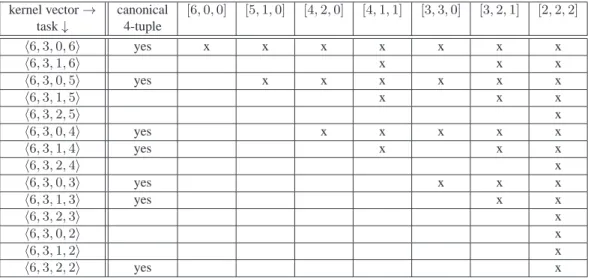
Examples All thehn, m, ℓ, ui-GSB tasks that are feasible with n = 6, m = 3 and u ≤ n = 6 are described in Table 1. Hence, the6 processes can decide up to 3 different values. The kernel vectors of each of these tasks is indicated, and these kernel vectors are listed according to their lexicographical order, from left to right.
As an example, the kernel vector[4, 2, 0] represents all the output vectors in which the most frequent value (that is1, 2 or 3) appears 4 times, the second most frequent value appears twice and the third possible value does not appear. As another example, the kernel set of the h6, 3, 0, 4i-GSB task is made up of five kernel vectors, namely, {[4, 2, 0], [4, 1, 1], [3, 3, 0], [3, 2, 1], [2, 2, 2]}. Let us finally observe that the balanced kernel vector [2, 2, 2] belongs to all tasks. Moreover, the GSB tasksh6, 3, 2, 5i, h6, 3, 2, 4i, h6, 3, 2, 3i, h6, 3, 0, 2i, h6, 3, 1, 2i and h6, 3, 2, 2i are
synonyms. The GSB tasksh6, 3, 1, 6i, h6, 3, 1, 5i and h6, 3, 1, 4i are also synonyms. Differently, while some tasks are “included” in other tasks (e.g., the kernel vectors associated with any task are included in the kernel set of the h6, 3, 0, 6i-GSB task, there are tasks that are not included one in the other (e.g., the h6, 3, 1, 4i-GSB and h6, 3, 0, 3i-GSB tasks).
kernel vector→ canonical [6,0,0] [5,1,0] [4,2,0] [4,1,1] [3,3,0] [3,2,1] [2,2,2]
task↓ 4-tuple h6,3,0,6i yes x x x x x x x h6,3,1,6i x x x h6,3,0,5i yes x x x x x x h6,3,1,5i x x x h6,3,2,5i x h6,3,0,4i yes x x x x x h6,3,1,4i yes x x x h6,3,2,4i x h6,3,0,3i yes x x x h6,3,1,3i yes x x h6,3,2,3i x h6,3,0,2i x h6,3,1,2i x h6,3,2,2i yes x
Table 1: Kernels ofhn, m, ℓ, ui-GSB tasks (with n = 6 and m = 3)
Remark It is important to notice that, while a set of kernel vectors can be associated with a task, not all sets of kernel vectors define a task. As an example, a simple look at Table 1 shows that the set of kernel vectors{[5, 1, 0], [4, 2, 0]} does not define a task.
4.2
The classes of ℓ-anchored, u-anchored and
(ℓ, u)-anchored tasks
This section presents subclasses of GSB tasks that provide us with a better insight into their family structure. More precisely, when we look at the tasks described in Table 1, we see that several GSB tasks are actually synonyms. Hence, it is important to have a single representative for all the GSB tasks that define the same task. This is captured by the notions ofℓ-anchored and u-anchored tasks.
Definition 6 (Anchoring). LetG be an hn, m, ℓ, ui-GSB task, G′be thehn, m, ℓ, min(n, u + 1)i-GSB task and G′′be thehn, m, max(0, ℓ − 1), ui-GSB task. G is ℓ-anchored if G and G′are synonyms.G is u-anchored if G and G′′are synonyms.G is (ℓ, u)-anchored if it is both ℓ-anchored and u-anchored.
Hence, ifG is ℓ-anchored, increasing the upper bound u does not modify the task and, if G is u-anchored, decreas-ing the lower boundℓ does not modify the task. Finally, (as we will see) an (ℓ, u)-anchored hn, m, ℓ, ui-GSB task is the hardest of the family ofhn, m, −, −i GSB tasks.
As an example let us consider the family ofh20, 4, −, −i-GSB tasks. The reader can easily check that h20, 4, 4, 8i is anℓ-anchored task, h20, 4, 2, 6i is a u-anchored task, h20, 4, 5, 5i is an (ℓ, u)-anchored task while h20, 4, 4, 6i is neither anℓ nor a u-anchored task.
It is easy to see that allhn, m, ℓ, ni (resp., hn, m, 0, ui) GSB tasks are ℓ-anchored (resp., u-anchored). These tasks are said to be trivially anchored.
Canonical representative of a GSB task Given anhn, m, ℓ, ui-GSB ℓ-anchored task, its canonical representative is thehn, m, ℓ, u′i-GSB task such that the hn, m, ℓ, u′− 1i-GSB task is not ℓ-anchored. A similar definition applies
for anu-anchored task. A task that is neither only ℓ-anchored nor only u-anchored, or that is (ℓ, u)-anchored, is its own representative.
As an example, let us look at Table 1. Theh6, 3, 2, 2i-GSB task, that is an (ℓ, u)-anchored task, is the representative for the six tasks associated with the single kernel vector[2, 2, 2]. The h6, 3, 1, 4i-GSB task, that is ℓ-anchored, is the representative for three tasks associated with the kernel set{[4, 1, 1], [3, 2, 1], [2, 2, 2]}. Finally, the h6, 3, 1, 3i-GSB task, that is not anchored, is its own representative: it is the only task associated with the kernel set{[3, 2, 1], [2, 2, 2]}. When considering Table 1 there are 7 canonical representative tasks. These canonical tasks are represented in Figure 1 where “A → B” means “A strictly includes B”. Let us notice that the representative h6, 3, 1, 3i-GSB task is not anchored.
these three tasks are trivially u-anchored
ℓ-anchored trivially u-anchored h6, 3, 1, 4i h6, 3, 0, 3i h6, 3, 1, 3i h6, 3, 0, 4i h6, 3, 0, 6i h6, 3, 0, 5i h6, 3, 2, 2i (ℓ, u)-anchored
Figure 1: Canonicalhn, m, −, −i GSB tasks are partially ordered
4.3
A characterization of ℓ-anchored and u-anchored GSB tasks
Let us remember that a task is feasible if its set of output vectorsO is not empty.
Theorem 3. LetT be a feasible hn, m, ℓ, ui-GSB task. T is ℓ-anchored if and only if u ≥ n − ℓ(m − 1).
Proof. Let us first suppose thatn − ℓ(m − 1) > u ≥ ℓ. As n − ℓ(m − 1) ≥ u + 1, there is a vector (with m entries) whose first entry is equal tou + 1 that is a kernel vector of the hn, m, ℓ, u + 1i GSB task. But, as u + 1 > u, this vector cannot be a kernel vector of thehn, m, ℓ, ui GSB task. It follows that the hn, m, ℓ, ui GSB task cannot be ℓ-anchored. Let us now suppose thatu ≥ n − ℓ(m − 1) ≥ ℓ and consider the counting vector [n − ℓ(m − 1), ℓ, . . . , ℓ] (with m entries). The sum of all its entries is n. Because the occurrence number n − ℓ(m − 1) is the only value higher than ℓ, it is the highest value that can appear in a kernel vector of both the hn, m, ℓ, ui task and the hn, m, ℓ, u + 1i for all u ≥ n − ℓ(m − 1). It follows that the hn, m, ℓ, ui and hn, m, ℓ, u + 1i GSB tasks are the same GSB task from which
we conclude thathn, m, ℓ, ui is ℓ-anchored. ✷T heorem3
Proof. The reasoning is similar to the one of Theorem 3. ✷T heorem4
The next corollary follows from the previous theorems.
Corollary 1. Letℓ ≤ n
m≤ u. The hn, m, ℓ, max(ℓ, n−ℓ(m−1))i-GSB task is ℓ-anchored, while the hn, m, max(0, n−
u(m − 1)), ui-GSB task is u-anchored.
4.4
The structural results
Lemma 4. LetT be any hn, m, ℓ, ui-GSB task. Let u′ ≥ u and T′ be thehn, m, ℓ, u′i-GSB task. We have S(T ) ⊆
S(T′).
Proof. The only difference betweenT and T′is the upper bound on the number of processes that can decide the same
value. If at mostu processes decide each value, then necessarily less than u′ processes decide each value, and thus
each output vector of thehn, m, ℓ, ui-GSB task T is also an output vector of the hn, m, ℓ, u′i task T′and consequently
S(T ) ⊆ S(T′).
✷Lemma4
Lemma 5. LetT be any hn, m, ℓ, ui-GSB task. Let ℓ′ ≤ ℓ and T′be thehn, m, ℓ′, ui-GSB task. We have S(T ) ⊆
S(T′).
Proof. The reasoning is similar to the one of Lemma 4. ✷Lemma5
The next theorem characterizes the hardest task of the sub-family ofhn, m, −, −i-GSB tasks. Let us remember that T1is harder thanT2ifS(T1) ⊂ S(T2).
Theorem 5. Thehn, m, ⌊n m⌋, ⌈
n
m⌉i-GSB task T is the hardest task of the family of feasible hn, m, −, −i-GSB tasks. Proof. As we consider only feasible tasks, we haveℓ ≤ n
m ≤ u. The proof follows then directly from Lemma 4 and
Lemma 5. ✷T heorem5
Let us observe that, givenn and m, the hn, m, ⌊n m⌋, ⌈
n
m⌉i-GSB task is not necessarily an anchored task. As an
example, theh10, 4, 2, 3i-GSB task is neither ℓ-anchored nor u-anchored while the h10, 5, 2, 2i-GSB task is (ℓ, u)-anchored.
Theorem 6. LetT be a feasible hn, m, ℓ, ui-GSB task, T 1 be the hn, m, ℓ′, ui-GSB task where ℓ′ = n − u(m − 1) and
T 2 be the hn, m, ℓ, u′i-GSB task where u′ = n − ℓ(m − 1). We have the following: (i) (ℓ′ ≥ ℓ) ⇒ S(T 1) ⊆ S(T ) and (ii)(u′ ≤ u) ⇒ S(T 2) ⊆ S(T ).
Proof. We prove the theorem for case(i). (The proof for case (ii) is similar.) Let us first show that the hn, m, ℓ′,
ui-GSB task is feasible, i.e.,ℓ′≤ n
m ≤ u. Let us first observe that, as the hn, m, ℓ, ui-GSB task is feasible, by assumption
we have mn ≤ u. Hence we only have to show that ℓ′ ≤ n
m which is obtained from the following (remember that
m > 1):
n/m ≤ u ⇔ n ≤ u · m
⇔ n(m − 1) ≤ u · m(m − 1) ⇔ n · m − u · m2+ u · m ≤ n
⇔ ℓ′= n − u · m + u ≤ n/m.
Asℓ′ = n − u(m − 1) ≤ n
m ≤ u, the size m vector [u, . . . , u, ℓ′] is a kernel vector of the feasible hn, m, ℓ′, ui GSB
task. Asℓ′ ≥ ℓ, this vector is also a kernel vector of hn, m, ℓ, ui GSB task, which concludes the proof for case (i).
✷T heorem6
Theorem 7. LetT be a feasible hn, m, ℓ, ui-GSB task and f () be the function f (ℓ, u) = (ℓ′, u′) where ℓ′= max(ℓ, n−
u(m − 1)) and u′ = min(u, n − ℓ(m − 1)). The canonical representative of T is the hn, m, ℓ
fp, ufpi-GSB task Tfp where the pair(ℓfp, ufp) is the fixed point of f (ℓ, u).
Proof. Let us first observe that, using the same reasoning as in Theorem 6, we haveℓ′ ≤ n m ≤ u
′, from which follows
thatTfp is feasible (Lemma 2). Moreover, due to the definition ofℓ′andu′, we also have0 ≤ ℓ ≤ ℓ′ ≤ mn ≤ u′ ≤
u ≤ n. We consider four cases.
• Case ℓ ≥ n − u(m − 1) and u ≤ n − ℓ(m − 1). We then have trivially ℓ′ = ℓ and u′ = u, from which we
conclude thatS(T ) and S(Tfp) have the same kernel vectors.
• Case ℓ′ = n − u(m − 1) > ℓ and u′ = u. Let us consider the kernel vector of T that has as many entries as
possible equal tou = u′. This means that this vector hasm − 1 entries equal to u = u′, and its last entry is equal
ton − u′(m − 1), i.e., equal to ℓ′. It follows thatS(T ) has no kernel vector with an entry equal to ℓ′′< ℓ′. We
conclude from that observation that the kernel vectors ofT are also kernel vectors of Tfp, i.e.,S(T ) = S(Tfp).
• Case ℓ′ = ℓ and u′ = n − ℓ(m − 1) < u. This case is similar to the previous one. Let us consider the kernel
vector ofT that has as many entries as possible equal to ℓ = ℓ′. This means that this vector hasm − 1 entries
equal to ℓ = ℓ′, and its last entry is equal to n − ℓ′(m − 1), i.e., equal to u′. It follows thatS(T ) has no
kernel vector with an entry equal tou′′> u′. Hence, the kernel vectors ofT are also kernel vectors of T fp, i.e.,
S(T ) = S(Tfp).
• Case ℓ′ = n − u(m − 1) > ℓ and u′= n − ℓ(m − 1) < u. This case is a simple combination of both previous
cases (one addresses the kernel vectors ofT with the greatest possible entries, and the other addresses the kernel vectors ofT with the smallest possible entries).
According to Theorems 3 and 4, neither thehn, m, ℓ′′, ui-GSB task with ℓ′′> ℓ′nor thehn, m, ℓ, u′′i-GSB task with
u′′< u′are synonyms ofT , which concludes the proof of the Theorem. ✷
T heorem7
5
Tasks solving tasks and non-determinism notions
So far we have defined GSB tasks and studied their internal combinatorial properties. We now focus on solvability is-sues and compare the computability power of GSB tasks against themselves and against agreement tasks. This section introduces four notions related to non-determinism which are used to compare the computability power between tasks. As the objects (instances of algorithms solving tasks) considered here are assumed to solve a task, they are one-shot objects, i.e., each process invokes the object operation at most once. Hence in our model we do not allow processes to locally simulate an object.
5.1
Non-deterministic objects
Let us consider a taskT = hI, O, △i and let X be an object that solves T .
1. X is fully-non-deterministic (FND) if for every I ∈ I and every execution in which processes invoke X with inputs inI, X may produce any O ∈ △(I). Thus, FND agrees with the usual assumption that an object solving a task is a “black-box” that may output any valid output configuration at any time.
2. X is unique-solo-deterministic (USD) if it behaves like an FND object except that there is a unique input value x ∈ [1, . . . , N ] such that X is deterministic in all solo-executions (executions in which only one process invokes X ) where the input is x, whatever the participating process.
3. X is deterministic (SOD) if it behaves like an FND object except that X is deterministic in all solo-executions, no matter the participating process and its input.
4. X is sequential-deterministic (SQD) if it behaves like an SOD object that additionally behaves deterministic in every non-concurrent invocation by a single process, namely, the output ofX in a non-concurrent invocation only depends on its internal state (just before the invocation) and the input.
To understand these definitions, consider an objectX that is invoked first by p, then q and r invoke it concurrently (afterp’s invocation has finished) and finally s invokes X alone. If X is FND, then it behaves non-deterministically in every invocation. IfX is USD, then X behaves non-deterministically in every invocation except p’s invocation, only if the input is the unique input for whichX is deterministic in solo-executions, otherwise X also behaves non-deterministically inp’s invocation. If X is SOD, then it behaves non-deterministically in every invocation except p’s invocation. And ifX is SQD, it behaves deterministically in the non-concurrent invocations of p and s, and it behaves non-deterministically in the concurrent invocations ofq and r.
5.2
Solvability
Note that an FND object that solves(n, k)-SA is necessarily SOD since there is only one possible output in solo-executions, by the definition of(n, k)-SA. Also observe that any two FND objects solving the same task have the same behavior, in the sense that both may produce the same outputs. However, this is not the case for other objects, SOD objects for example: it is possible that an SOD object outputsy in solo-executions with input x, and another SOD object outputsz 6= y in solo-executions with the same input x. Below we consider algorithms that solve a task from any SOD (resp. USD or SQD) object.
LetT and T′be tasks. For ZZZ∈ {FND, USD, SOD, SQD}, we say that T ZZZ-solves T′, denotedT → ZZZ T′,
if there is a wait-free algorithmA that solves T′ from read/write registers and multiple copies of any ZZZ objectX
that solvesT . It is required that A solves T using any ZZZ object X , however, we do not exclude the possibility that processes have an input informing some properties aboutX (for example, the outputs the objects may produce in solo-executions). The statementT 9ZZZ T′means¬(T →ZZZ T′).
Given two tasks T and T′, if there is an algorithmA that solves T′ from FND objects that solvesT , then we
can obtain an algorithmB that solves T′ by replacing every object solvingT in A with a USD object that solves T .
The resulting algorithmB solves T′because USD objects are indeed FND objects with the property that they behave
deterministically in certain solo-executions. Hence the set containing all possible outputs an USD object solvingT may produce, is a subset of the set containing all possible outputs an FND object solvingT may produce. Thus, if T →FND T′thenT →USD T′. Similarly, ifT →USDT′, thenT →SOD T′, and ifT →SOD T′, thenT →SQD T′.
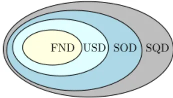
Therefore, the four relations induce a solvability hierarchy: for a GSB taskT , let SZZZ be the set containing all
tasks thatT can ZZZ-solve, ZZZ ∈ {FND, USD, SOD, SQD}; hence SF N D⊆ SU SD⊆ SSOD⊆ SSQD(see Figure
2).
USD SOD SQD FND
Figure 2: A solvability hierarchy
5.3
On the notions of non-determinism
For proving our computability results in subsequent sections, we consider objects with different non-determinism assumptions, from FND objects to SQD objects. But why do we consider objects holding deterministic properties? Is this an “artificial" way of boosting the computational power of GSB tasks? Arguably, no.
First, the results relating set agreement and renaming in [36] consider different assumptions on the non-deterministic behavior the objects can exhibit. Although it is not explicitly stated, the possibility result that(n−1)-set agreement can
implement(2n − 2)-renaming, assumes (n − 1)-set agreement objects that are FND. And the impossibility result that, for oddn, (2n − 2)-renaming cannot solve (n − 1)-renaming, holds for (2n − 2)-renaming objects that are SQD (see Appendix B for a detailed explanation). The next theorem shows that the SQD assumption in the impossibility result is reasonable since the computability power of FND objects solving GSB task is null when measured against agree-ment tasks, or more generally against any read/write unsolvable task without the requireagree-ment of index-independent algorithms.
Theorem 8. Let T be a GSB task and T′ be any task which is read/write unsolvable without the requirement of index-independent algorithms. Then,T 9F N DT′.
Proof. LetT = hI, O, △i. Pick any O ∈ O. Recall that for every I ∈ I, △(I) = O. Suppose by contradiction that there is a read/write wait-free algorithmA that solves T′ from FND objects solvingT . Let S be the set containing
all possible executions ofA. Consider the algorithm B obtained from A by replacing each object solving T with a local function that always returnsO[i], for every process pi. The fact thatA uses only FND objects implies that every
execution ofB belongs to S. Thus, B must be wait-free and solve T′, otherwiseA would not be wait-free nor solve T′.
Note thatB is not index-independent, however this is not a problem because solutions to T′ do not have to hold that
property. AlgorithmB uses only read/write operations, contradicting that T′is read/write unsolvable.
✷T heorem8
Second, from our perspective, in the task context and without randomness, it is reasonable to assume the non-determinism of shared objects is completely and only due to the possible interleavings of computation steps. Therefore, we believe that the natural way to compare the power of tasks is via SQD objects. For the interested reader, [13] presents a wide discussion about the concept of non-determinism and its relation with concurrency in distributed computing.
Another reason to consider SQD objects is the following. Some tasks have the property that any object that solves one of them is necessarily SQD. This is implied by the very definition of the task. Test&set, for example, has this property. If a process calls alone a test&set object, then the process must get winner. In contrast, if two or more processes concurrently call a test&set object, there is no certainty about which process is going to get winner. Moreover, in subsequent invocations, a process must get loser.
As already explained, for us, the natural way to compare the power of tasks is via the SQD-solvability relation, →SQD. However, our possibility results hold for FND or USD objects, while our impossibility results hold for SOD
or SQD objects.
5.4
Transitivity of FND, USD, SOD and SQD-solvability
FND objects Consider three tasksT1, T2andT3. Suppose there is an algorithmA that FND-solves T2 fromT1.
SinceT1objects inA are FND, it follows that A is indeed an FND object that solves T2. Now, if there is an algorithm
B that FND-solves T3fromT2, then we can replace eachT2object inB with an instance of A. Therefore, we have
that ifT1→FND T2andT2→FND T3, thenT1→FND T3.
SOD and SQD objects Similarly, if there is an algorithmA that SOD-solves T2fromT1, thenA is SOD because
in every solo-execution the participating process calls SOD objects (which behave deterministically since all calls are indeed solo-executions) and accesses read/write registers without concurrency. HenceA behaves deterministically in solo-executions. Therefore, if there exists an algorithm that SOD-solvesT3fromT2, we can replace eachT2object
with an instance ofA. We conclude that if T1→SOD T2andT2→SOD T3, thenT1 →SOD T3. A similar argument
shows the transitivity property of the→SQD relation.
USD objects The case of→USD is a bit more tricky because it is possible that in an algorithmA that USD-solves
T1fromT2, for every inputx, in every solo-execution with input x, the participating process invokes some T1objects
with inputs for which the objects behave non-deterministically, and henceA may behave non-deterministically in every solo-execution. However, Lemma 6 below shows that given an USD object that solves a GSB taskT , using read/write registers and the USD object, one can construct an SOD object that solvesT . As explained below, this lemma implies that ifT1andT2are GSB tasks, andT1→USD T2andT2→USD T3, thenT1→USD T3.
Lemma 6. LetT be any GSB task. If there is an USD object that solves T , then there is an SOD object that solves T .
Proof.
LetA be any read/write wait-free comparison-based algorithm that solves (2n − 1)-renaming, i.e., hn, 2n − 1, 0, 1i-GSB ([21] presents several such algorithms). Consider a processpiand letE be a solo-execution of A in which pi
participates. From the fact thatA is comparison-based we get that the output value of pi inE is not a function of
its input value (intuitively, becausepionly uses comparison operations). Thus in every solo-execution, no matter its
input,pi always gets the same output value, sayλ. As pi getsλ in a solo-execution and A is index-independent, we
conclude that in any solo-execution in whichpjparticipates,j 6= i, whatever its input value, pjgetsλ. Let us assume,
w.l.o.g.,λ = 1.
Consider now an USD objectX that solves T , and let x be the input such that for every pi,X is deterministic in
a solo-execution ofpiwith inputx. Let us assume, w.l.o.g., x = 1. Using A and X , we implement an SOD object
that solvesT . The idea is to use A as a preprocessing stage in order that in every solo-execution, the participating process always, invokesX with input 1, whatever the input. Each process first invokes A using its original input. Then, a process uses as input toX the value it gets from A and finally outputs the value it receives from X . Note that in every solo-execution, the participating process callsX with input 1, thus the resulting object is SOD because X is
deterministic in solo-executions with input 1. ✷Lemma6
By Lemma 6, if we have an USD object that solvesT1, we can build an SOD object that solvesT1. And as
explained in the previous section,T1 →USD T2impliesT1 →SOD T2. Similarly, Lemma 6 andT2→USD T3imply
T2 →SOD T3. By transitivity of→SOD,T1 →SOD T3. Finally, consider an algorithmA that SOD-solves T3from
T1. Lemma 6 implies that given an USD objectX that solves T1, it is possible to replace each SOD object inA with
a copy ofX and read/write registers in a way that A stills solves T3. Therefore,T1→USD T3.
6
Solvability of GSB tasks
Recall that for ahn, m, ~ℓ, ~ui-GSB task T = (I, O, ∆), we have that ∆(I) = ∆(I′) = O, for any two input vectors
I, I′. Thus, at first sight, it could seem that a trivial solution forT could be to simply pick a predefined output vector
O ∈ O, and always decide it without any communication, whatever the input vector. This is not the case because of the index-independence requirement. In fact, there are GSB tasks that are not wait-free solvable (with any amount of communication).
This section investigates the difficulty of solving GSB tasks. In particular, it considers read/write solvable GSB tasks, i.e., for which there exists a wait-free algorithm based only on read/write registers.
As we shall see, the universe of GSB tasks includes trivial tasks that can be solved without accessing the shared memory, and universal tasks, that can be used to solve any other GSB task. In between, there are wait-free solvable tasks, as well as non-wait-free solvable tasks.
6.1
Hardest GSB tasks: Universality of the
hn, n, 1, 1i-GSB task
When considering the GSB family of tasks, an interesting question is the following: is there a universal GSB task? In other words, is there a GSB task that allows all other GSB tasks onn processes to be solved? The answer is “yes”. We show in the following that the perfect renaminghn, n, 1, 1i-GSB task allows any task of the family to be solved. Hence, perfect renaming is universal for the family ofhn, −, −, −i-GSB tasks.
As we will see with Corollary 5, thehn, n, 1, 1i-GSB task (perfect renaming) is not a wait-free solvable task [7]. We present a novel proof of this impossibility result.
Theorem 9. Any (feasible)hn, m, ~ℓ, ~ui-GSB task can be FND-solved from the perfect renaming hn, n, 1, 1i-GSB task.
Proof. Let us first observe that thehn, n, 1, 1i-GSB task has a single kernel vector, namely, [1, . . . , 1]. Given an algorithm solving that task, let deci be the output at processpi.
To solve the symmetrichn, m, ℓ, ui-GSB task, the processes execute an algorithm solving the hn, n, 1, 1i-GSB task, and a processpiconsiders outputi = ((deci− 1) mod m) + 1 as its output. The corresponding kernel vector
form output values is then [⌈m n⌉, . . . , ⌈ m n⌉, ⌊ m n⌋, . . . , ⌊ m
n⌋]. By the feasibility assumption, we have ℓ ≤ m
n ≤ u. As
ℓ and u are integers, we have ℓ ≤ ⌊m n⌋ ≤ ⌈ m n⌉ ≤ u. The vector [⌈ m n⌉, . . . , ⌈ m n⌉, ⌊ m n⌋, . . . , ⌊ m n⌋] is consequently a
kernel vector of thehn, m, ℓ, ui-GSB task.
To solve the asymmetrichn, m, ~ℓ, ~ui-GSB task, we first consider the set of output vectors O. We then order these vectors in the same, deterministic way, and pick the first one. LetV be this vector of the hn, m, ~ℓ, ~ui-GSB task. We use then the same vectorV for all processes. Let decibe the value obtained by processpiin thehn, n, 1, 1i-GSB task.
A processpi then considersV [deci] entry as its output outputi with respect to thehn, m, ~ℓ, ~ui-GSB simulated task.
Because thehn, n, 1, 1i-GSB task has a single kernel vector [1, . . . , 1], it follows that each entry of V is chosen by only a single process. This satisfies the specification of thehn, m, ~ℓ, ~ui-GSB task, which concludes the proof of the
theorem. ✷T heorem9
6.2
Easiest GSB tasks: Solvability of GSB tasks with no communication
This section identifies the easiest of all the GSB tasks, namely those that are solvable with no communication at all. This is under the assumption that the domain of possible identities is of size2n − 1 (see Theorem 1). It is easy to see that any feasible GSB task wherem = 1 is solvable without any communication (a single value can be decided). The next theorem characterizes the communication-free GSB tasks whenm > 1.
Theorem 10. Consider anhn, m, ℓ, ui-GSB task T where m > 1. Then, T is read/write solvable with no
communi-cation if and only if(ℓ = 0) ∧ (⌈2n−1 m ⌉ ≤ u). Proof. Let us first assumeℓ = 0 and u = ⌈2n−1
m ⌉ (increasing u makes the problem even easier). Recall that the
identities of the processes are taken from1..2n − 1. Let us deterministically partition the 2n − 1 identities into m groups,G1, . . . , Gm, so that no group has more than⌈2n−1m ⌉ elements and no group has less than ⌊2n−1m ⌋ elements.
Letδ be the deterministic function that maps identities in group Gi toi(the partitioning and δ are known by every
process). To solveT with no communication, each process pioutputsδ(idi) and we have that each value x ∈ [1..m]
is decided by at most⌈2n−1m ⌉ processes.
For the other direction, let us first consider anhn, m, ℓ, ui-GSB task T with m > 1 and u < ⌈2n−1m ⌉. Suppose, by way of contradiction, that there is an algorithmA that solves T with no communication. The algorithm implies a decision functionδ that assigns to each identity x in 1..2n − 1, an output value δ(x) in 1..m. The value δ(x) is the decision produced by a process when it starts with identityx, without any communication. Define groups Giby
putting in the same group identitiesx, x′ wheneverδ(x) = δ(x′). For any partition of the set of identities, the size
of the biggest group is at least⌈2n−1
m ⌉. The task specification requires that for each i, |Gi| ≤ u < ⌈ 2n−1
m ⌉, which is
impossible.
Let us now consider anhn, m, ℓ, ui-GSB task T with m > 1 and ℓ > 0. For any partition of the set of identities, asm ≥ 2, the size of the smallest group is at most ⌊2n−1
m ⌋ ≤ n − 1. The task specification requires that, for each i,
|{pj | δ(idj) = i}| ≥ ℓ ≥ 1. Because there are n − 1 identities not corresponding to any process and the size of the
smallest group obtained from the partitioning is at mostn − 1, it follows that it is possible that no process belongs to
some group, which concludes the proof. ✷T heorem10
Let us callx-bounded renaming the hn, ⌈2n−1x ⌉, 0, xi-GSB task. This task can easily be solved, namely, process pidecides the value⌈idxi⌉.
Corollary 2. Thex-bounded renaming hn, ⌈2n−1x ⌉, 0, xi-GSB task is read/write solvable with no communication.
The next corollary is an immediate consequence of Theorem 10 whenm = 2 and ℓ = 1.
Corollary 3. The WSBhn, 2, 1, n − 1i-GSB task is not read/write solvable without communication.
When m = 2n − 1 in Theorem 10, we have the trivial hn, 2n − 1, 0, 1i-GSB, which is actually the classical (non-adaptive)(2n − 1)-renaming problem for which many solutions have been proposed (e.g., [5, 8, 15]; see [21]
![Figure 9: Replacing an hn, n − x, [1, .., 1, x + 1], [1, .., 1, x + 1]i-GSB object X in A (code for p i ).](https://thumb-eu.123doks.com/thumbv2/123doknet/11335326.283734/38.892.291.616.216.373/figure-replacing-hn-n-gsb-object-x-code.webp)
![Figure 10: A wait-free implementation of a splitter object (code for p i ) [47, 50].](https://thumb-eu.123doks.com/thumbv2/123doknet/11335326.283734/39.892.372.549.524.677/figure-wait-free-implementation-splitter-object-code-p.webp)
