Importance relative des producteurs primaires sur la production globale du lac Saint-Pierre, un grand lac fluvial du Saint-Laurent

Importance relative des producteurs primaires sur la production globale du lac Saint-Pierre, un grand lac fluvial du Saint-Laurent

par Chantai Vis

Département de sciences biologiques faculté des arts et sciences

Thèse présentée à la faculté des études supérieures en vue de l’obtention du grade de

Fhilosophiœ Doctor (Ph. D.)

Juin 2004

Z) ‘•

1

de Montréal

Direction des bibliothèques

AVIS

L’auteur a autorisé l’Université de Montréal à reproduire et diffuser, en totalité ou en partie, par quelque moyen que ce soit et sur quelque support que ce soit, et exclusivement à des fins non lucratives d’enseignement et de recherche, des copies de ce mémoire ou de cette thèse.

L’auteur et les coauteurs le cas échéant conservent la propriété du droit d’auteur et des droits moraux qui protègent ce document. Ni la thèse ou le mémoire, ni des extraits substantiels de ce document, ne doivent être imprimés ou autrement reproduits sans l’autorisation de l’auteur.

Afin de se conformer à la Loi canadienne sur la protection des renseignements personnels, quelques formulaires secondaires, coordonnées ou signatures intégrées au texte ont pu être enlevés de ce document. Bien que cela ait pu affecter la pagination, il n’y a aucun contenu manquant. NOTICE

The author of this thesis or dissertation has granted a nonexclusive license allowing Université de Montréal to reproduce and publish the document, in part or in whole, and in any format, solely for noncommercial educational and research purposes.

The author and co-authors if applicable retain copyright ownership and moral rights in this document. Neither the whole thesis or dissertation, nor substantial extracts from it, may be printed or otherwise reproduced without the author’s permission.

In compliance with the Canadian Privacy Act some supporting forms, contact information or signatures may have been removed from the document. While this may affect the document page count, it does not represent any loss of content from the document.

Faculté des études supérieures

Cette thèse intitulée:

Importance relative des producteurs primaires sur la production biologique totale du lac Saint-Pierre, un grand lac fluvial du Saint-Laurent

présentée par: Chantai Vis

a été évaluée par un jury composé des personnes suivantes:

Antoneila Cattaneo président—rapporteur Richard Carignan directeur de recherche Christiane Hudon codirectrice de recherche Bemadette Pinel-Alloul membre du juiy Robert G. Wetzel examinateur externe Pierre André

SOMMAIRE

Ces dernières années, des fluctuations importantes dans les niveaux d’ eau du système des Grands Lacs - $aint-Laurent ont attiré l’attention sur le fait que ces

changements pouvaient avoir des impacts écologiques importants dans ces systèmes. Cependant, le manque de données, en particulier sur les communautés situées à la base des réseaux trophiques tels que les producteurs primaires, limite actuellement notre capacité à comprendre le fonctionnement de ces écosystèmes et à prédire leur réponse face à des fluctuations de niveaux d’eau. Cette thèse quantifie, à grande échelle, la production primaire des macrophytes, des épiphytes et du phytoplancton durant deux années avec des niveaux d’eau opposés, dans le Lac Saint-Pierre, un grand (--3OO km2) lac fluvial du fleuve Saint-Laurent.

Une comparaison des méthodes d’estimation de la biomasse et de la distribution des plantes aquatiques émergentes et submergées à l’échelle du lac montre que l’utilisation de modèles empiriques intégrés dans un système d’information géographique ($1G) se révèle efficace pour déterminer la distribution spatiale des macrophytes pour tous les types d’habitats au Lac Saint-Pierre. Une méthode de correction pour les modèles de production primaire phytoplanctonique a été développée pour permettre une application spatiale de ces modèles dans des milieux optiquement complexes tels ceux du fleuve Saint-Laurent. Le taux de photosynthèse des algues épiphytiques est fortement lié à la biomasse algale, et moindrement influencé par la lumière et la température. La distribution de la biomasse des macrophytes et des épiphytes et la réponse photosynthétique en fonction de la profondeur a un effet important sur l’estimation de la production des épiphytes à l’échelle du système. En général, les algues filamenteuses utilisent plus efficacement la lumière que les algues attachées, leur donnant ainsi un avantage compétitif face à des changements de niveau d’ eau.

Une analyse de la production primaire totale à l’échelle du lac indique qu’une diminution du niveau d’eau d’un mètre en 2001, comparativement à 2000, a entraîné une réduction de la superficie des marais de 50%, une augmentation dramatique de la production par le phytoplancton dans la zone d’eau libre de 60%, une augmentation de la biomasse et de la production des algues filamenteuses, ainsi qu’une hausse de la production primaire globale de 20%, soit l’équivalent de 5000 tonnes métriques de

carbone. Cependant, la contribution relative des producteurs primaires à l’échelle du lac a été peu affectée par un abaissement du niveau d’eau, en raison de l’hétérogénéité spatiale du système. Une étude spatiale de la production primaire indiquait des variations dans la distribution et dans le type de producteurs entre les années. Cette étude représente la première estimation de la production primaire totale du Lac Saint Pierre par type de producteur, et l’une des premières estimations quantitatives de production autotrophe totale dans une grande rivière. Les résultats de cette thèse soulignent l’importance d’incorporer l’hétérogénéité spatiale de la production autotrophe pour une vision intégrée du fonctionnement des grandes rivières.

Mots clés: production primaire, rivière, fleuve, SIG, phytoplancton, macrophytes, épiphytes, niveau d’eau

SUMMARY

In recent years, fluctuating flow and water levels in the Great Lakes—St. Lawrence River system have drawn attention to the potential ecological impacts of lower water levels on this system. Total primary production of the St. Lawrence River remains largely unlmown, and because primary producers are at the base of the food chain, this lack of information hinders our capacity to understand the flow of carbon and to predict the consequences of altered water levels on ecosystem processes. This thesis examines the primary production of macrophytes, epiphyton and phytoplankton over a 2-year period with contrasting water levels in Lake St. Pierre, a large (—30O2)

fluvial lake ofthe $t. Lawrence River (Canada).

A comparison of methods used to determine the distribution and biomass of aquatic macrophytes showed that empirical models integrated in a GIS-framework provided the most adequate estimation of macrophyte biomass across the entire range of riverine habitats in Lake St. Pierre. A general model to correct daily phytoplankton primary production estimates for errors arising from variable optical depths was developed to allow for increased spatial and temporal modelling of algal production in diverse, shallow water systems. Epiphyton specific-productivity in Lake St. Pierre was related to biomass, light and temperature and areal estimates of epiphyton production were found to be strongly dependent on vertical variations in light and biomass within macrophyte stands. Filamentous algal mats utilised light more efficiently than attached epiphytes, conferring a competitive advantage over attached forms under conditions of lower water levels.

Analyses of whole-system primaly production revealed that macrophytes and epiphyton were responsible for roughly haif of annual autotrophic production in Lake St. Pierre. Under low water levels in 2001, coverage by wetted emergent marsh habitats decreased by 50%, phytoplankton production in the open water zone increased by 60%, filamentous algal biomass and production increased dramatically and whole-system carbon production increased by 20 %, or roughly 5000 mt C. Changes in the relative contributions of primary producers to annual production at the scale of the lake between years were relatively minor. Examination of the spatial distribution of production revealed important shifis in the location and type of primaiy producers. This study

represents the first estimate of primary production and of the relative contributions of the various producing communities in Lake $t. Pierre and one of the first quantitative estimates of whole-system primary production in a large river system. Resuits of this study underline the importance of considering spatial variations in autotrophic production for a comprehensive view of the functioning of large river systems.

Keywords: primary production, large river, GIS, phytoplankton, macrophytes, epiphyton, water level

TABLE DES MATIÈRES

Sommaire III

Summary V

Table des matières VII

Liste des tableaux X

Liste des figures XV

Remerciements XXII

Dédicace XXIII

Introduction générale 1

Le rôle de la production primaire dans la structure et le fonctionnement des

écosystèmes 1

L’ importance relative des producteurs primaires dans différents milieux

aquatiques 3

Importance du régime hydrique des grandes rivières 5

Site d’étude 6

Objectifs et sommaire des chapitres 7

Bibliographie 9

Chapitre 1. An evatuation ofapproaches used to determine the distribution and biomass ofemergent and submerged aquatic macrophytes over large spatial scales.

Abstract 17 Introduction 17 Study area 18 Methods 22 Resuits 29 Discussion 29 Acknowledgements 37 References 37

Chapitre 2: Estimating daiÏy phytoplankton production in shallow watersystems.

correctingfor variable optical depths.

Abstract 42 Introduction 42 Methods 44 Resuits 51 Discussion 59 Acknowledgements 63 References 63

Chapitre 3. Variations in photosynthesis and respiration by epzphyton andfilamentous algal mats in afluvial lake ofthe St. Lawrence River: implications on estimates ofareal epzhyton production Abstract 67 Introduction 67 Methods 69 Resuits 77 Discussion 90 Acknowledgernents 101 References 102

Chapitre 4. Frimaiy production by macrophytes, epiphyton andphytoplankton in a large fluvial lake of the St. Lawrence River under dfferent water level conditions

Abstract 109 Introduction 110 Methods 112 ResuÏts 132 Discussion 156 Acknowledgements 164 Literature cited 164

Conclusions générales .173

Annexe I. Relations entre la photosynthèse et la lumière(P-I) pour les communautés

épiphytiques du Lac Saint-Pierre en 2000 et 2001 179

Annexe II. Relations entre la photosynthèse et la lumière (P-I) pour le phytoplancton du

Lac Saint-Pierre en 2000 et 2001 184

Annexe III. Informations supplémentaires sur les macrophytes submergées et

émergentes qui ont servi au calcul de la production épiphytique 187

Annexe IV. Données physiques, chimiques et biologiques mesurés au Lac St. Pierre en

LISTE DES TABLEAUX

Chapitre 1

Table 1 Physical, chemical and biological characteristics (mean+ 1 S.E.) of the

different water masses in Lake St.Pierre 22

Table 2 Summary of the macrophyte growth form groups used in the

comparison among methods 28

Table 3. Accuracy of predicted occurrence of macrophyte growth form groups (group 1-5) for each method. The observed total is the number of field data pixels for each macrophyte growth form group, the predicted total is the number of predicted pixels for each group and the correct total is the number of correctly classified pixels for each group. four measurements of accuracy are used: Percent agreement, Kappa statistic K, Producer’s and Consumer’s accuracy. (see

Methods for more information) 34

Chapitre 2

Table 1. Data used in the example of the optical depth correction model applied to Lake St. Pierre, St. Lawrence River (June 2000). Mean biomass (B), light attenuation (K) and theoretical euphotic depth (Zeu) calculated as 4.6 / K are presented for each water mass. Based on the mean depth of each water mass polygon, the ratio of theoretical euphotic depth to mean depth, euphotic zone production (Pz,) estimated from the composite variable 0.O32XBZeuI0T, areal production corrected for optical depth (Pz,t) using Eq. 1, and the decrease in areal production resulting from the correction were calculated. A surface irradiance (In) of 40 mol quanta m2 d1 and a water temperature (T) of 16°C were used in ail

Chapitre 3

Table 1. Range in environrnental variables (mean ± s.d.) observed at the study sites in Lake St. Pierre between June and September of 2000 and 2001. Significant differences between sites are indicated by different lowercase letters;

a,

b

Table 2. Summary statistics for photosynthetic pararneters, respiration rate, mean sampling depth and light conditions of periphyton and filamentous algal mats (FAM) in Lake St. Pierre. Pmaxis the maximum rate of light-saturated gross photosynthesis, a is the initial siope, ‘k is the saturation PAR and Rcom is the

cornmunity dark respiration rate calculated per unit biomass (Chi a) or per unit surface area of substratum (rn2) for periphyton. Biornass is measured in mgChl a m2 for periphyton and in mgChl a m3 for FAM. Light is the in situ percentage of surface inadiance at sampling depth calculated from light attenuation

coefficients (K) 82

Table 3. Resuits of stepwise linear regressions relating 1og10-transformed maximum photosynthesis rates to environrnental factors (in situ light, daily PAR and recent irradiance history, temperature) and epiphyton biomass (Chl a, mg Chi a m2). Abbreviations for environmental factors are: water temperature (Temp, °C) and percentage of incident light at sampling depth (Light,

%),

sampling depth (Z) 89

Table 4. Areal epiphytic production (mgC m2 d’) calculated for variable vertical distribution of epiphyton biomass and photosynthetic response in hypothetical macrophyte stands of various types (f igure 7, A-D). Epiphyton biomass (mgChl a m2 (0.2m depth)1) is summarised in the table as the ratio of biomass in the top versus bottom 0.2 m stratum of the water column. For each biomass scenario (A-D) depicted in f igure 7, areal epiphytic production was

calculated assuming a constant photosynthetic response with depth (PmaxB = 1.2

mgC (mgChl a) W’, c = 0.007 mgC (rngChl a’) W’(tmoF’ nï2 s1)

rn’)), and a

variable photosynthetic response in the top versus bottom portion of the stand (Prnax - 1.6 : 0.8 mgC (mgChl a’) lï’, a’3 - 0.003:0.0011 mgC (mgChl a’) W m2 1) 1 for different light attenuations in the water column. Percent change in areal production relative to the situation of uniform distribution of epiphyton biomass and a constant photosynthetic response with depth are

presented for each scenario 95

Table 5. Photosynthetic parameters observed in various whole-assemblage periphyton studies. Values indicated means ± SE when reported or ranges in values (minimum and maximum). Abbreviations and units are as follows: maximum gross photosynthesis (PmaxB, _{mgC (mgChl a’) 1ï1), initial siope (cf,} mgC (mgChl a1) lï’()lmol’ m2 1) 1), saturation parameter (‘k, jimol quanta m2 s1), _{and biomass in mgChl a per m2 of substratum 9$}

Chaptitre 4

Table 1. Landsat TM images used to rnap the distribution of the four main water masses ofLake St. Pierre in spring (May) and summer (June to October) 2000 and 2001. Daily water level (m, GLD$5) are presented for Lake St. Pierre

gauging station Curve no.2 for eachimage 122

Table 2. Multiple regression models predicting maximum submerged aquatic vegetation SAV biomass (Bmax) in the open water zone, light attenuation coefficients (Ktotai) and epiphyton areal production (epiAP) from environmental variables. Abbreviations are as follows: Zw is the wave effect depth (m), Bt is the seasonal macrophyte biomass (g DM m2), KZ is optical depth (light

attenuation coefficient K (m’) x water depth (Z)), and 1 is total daily inadiance (mol quanta m2 dj. Water mass was entered as a dummy variable representing

the 3 (macrophyte mode!) or 4 water masses of Lake St.

Pierre’ 124

Table 3. Parameter estimates for the non-linear regression mode! predicting differences in the surface water elevation between the upstream and downstream

of Lake St. Pierre (siope) as a function of day (plant growth and tidal effects) and

wind variables. Julian is the Julian day within each year and Date is the number

of cumulative days starting from 1 January 2000 (Date = 1). WindW$W is a proxy for wind effect combining average wind speed and direction (see Eq.2). The sum of square error (S SE) and number of observations (n) of the mode! are

indicated 128

Table 4. Summary of annual flow and ftow-related variables (surface area and

average depth) of the four water masses of Lake St. Pierre for 2000 and

2001 136

Table5. Comparison of the mean (S.D.) physical and chemical properties of the

four water masses in Lake St. Pierre between 2000 and 2001. The following

abbreviations were used; light attenuation coefficient of water column alone

(Kwater), of the water colunm including shading effects of plants (Ktotai) and

Chlorophyli a concentration (Chia). Paired t-tests (by water mass and week)

were performed to test the significance of differences between years. n = 10

except for the mix and south water masses in 2000 where n =$ or 9. $uspended

solids and color were only measured in 2001 137

Table 6. $ummary of mean depth (m), surface area (km2) and maximum aboveground biomass of aquatic vascular vegetation (g dry mass m2) in Lake St.

Pierre in 2000 and 2001. Mean biomass ($.E, n) of wetland classes (marsh,

including mean maximum biomass (min-max) of $AV in open water habitat, were derived from GIS-based modeling. Approximate error on total biomass

were calculated from Monte Carlo simulations 141

Table 7. Comparison of the biomass-specific photosynthetic and respiration rates of phytoplankton and epiphyton measured simultaneously in June, August and September of 2000 at sites located in the north and central water masses. p13 _{is the maximum rate of light-saturated gross photosynthesis, a is the initial} siope of the P-1 curve, ‘k is the saturation PAR and Rcom is dark community

respiration rates. Volumetric (phytoplankton) and substratum-specific (epiphyton) biomass were measured as Chia. Values are means± standard error,

(minimum and maximum) and n =6. 145

Table 8. Estimate of the biomass (mean, min-max) and production by filamentous algal mats (metaphyton) in Lake St. Pierre in 2001. n 19 151

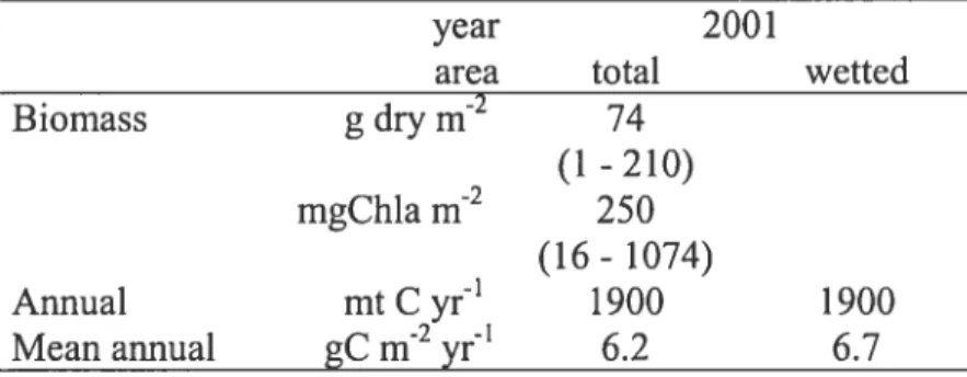
Table 9. Carbon budget for primary production in Lake St. Pierre for 2000 and 2001. Approximate enor on annual production were based on Monte Cario

LISTE DES FIGURES

Chapitre 1

Figure 1. Map of Lake $t. Pierre, St. Lawrence River, its major tributaries and the distribution of its water masses. The location of the fleld survey sites (circles) and the boundaries of each water mass (hatchcd white unes) are indicated on a black and white satellite image (Landsat TM from September 16, 1988). The water masses are from north to south: the north shore, the navigation

channel, the central area and the south shore 21

Figure 2. Box plots of (A) Daily water levels and (B) Suspended matter concentrations for the years compared in the study (1990, 1993, 1994, 1996,

2000) 31

Figure 3. Distribution of macrophyte growth form groups estimated by five methods (A-E) and map of the field data for Lake St. Pierre. Areas compared in this study are indicated on the remote sensing and field data map (solid line: CD

+ 1m water limit and dotted une: deep water zone). Thatched area flot surveyed

by echo sounding 33

Chapitre 2

Figure 1. Map of the Lake St. Pierre, St. Lawrence River (Quebec, Canada) showing the distribution of its major water masses. The boundaries of each water mass (solid white une) were outlined on a black and white Landsat TM image from September 21, 1984 and are from north to south: the north, mix, central and south water masses. The dotted une is the location of the

Figure 2. A bathymetric profile of a cross-section of Lake St. Pierre, St. Lawrence River. Boxes represent euphotic zone primary production in various regions of the lake; hatched area is the overestimation of areal phytoplankton production if estimates are uncorrected for optical depth. The distribution of the

major water masses are indicated 49

Figure 3. Relationship of integrated daily production (Pz,) and optical number

(K x Z; light affenuation times integration depth). Pz,t was calculated at

increasing depths by increments of 0.1 m between the surface and 4 m and by increments of 1 m between 4 m and 10 m, for the median observations in photosynthetic parameters and light in the St. Lawrence River (open circles). Representative values of the median conditions in the St. Lawrence River used

were; Pmax = 11 mg C m3 h’, = 12 mg C mol quanta1 m2), light attenuation

K= 1.3 m1 and daily surface irradiance 1 = 40 mol quanta m2 d’). The data

were fit to a generaÏized von Bertalanffï growth equation (solid une: see text for

details) 54

Figure 4. Observed and predicted euphotic zone primary production (mgC m2

d1) for the St. Lawrence River. Predicted production was calculated from A) the original composite variable linear regression mode! (Eq. 1) applied to the St. Lawrence River data and from B) the modified composite variable linear

regression model which includes a fourth term, water temperature (T). The

intercepts of both linear regression models were flot significantly different from

zero (p< _{0.05, $tudent’s T-test using asymptotic standard errors) and, thereby not}

used in the models 56

Figure 5. Estimates of areal phytoplankton primary production uncorrected (euphotic zone primaiy production) (A) and corrected for variable optical depth

(B) and the percent correction

(%

Figure 6. Comparison of the depth correction modet fit to data from the St. Lawrence River with the mode! fit to data from two other aquatic systems, a series of Canadïan Shield Lakes (dash-dotted une) and Chesapeake and Delaware

Bays (dashed une). Median values of photosynthetic parameters and light

conditions for Canadian Shield Lakes and Chesapeake and Delaware Bays were calculated from data presented in Carignan et al. 2000 and Harding et aI. 1986,

respectively. The estimates of the fitted constant are presented on the figure.

The depth correction model based on a third-order polynomial of Brawley et al.

2003 is also shown (dotted une) 62

Chapitre 3

Figure 1. Map of study sites !ocated in Lake St. Pierre, St. Lawrence River overlying a black and white Landsat TM image (21 September 1984) which shows the distribution of the major water masses. Site I (north water mass) and

2 (central water mass) were sampled in 2000 and 2001, site 3 (south water mass)

was added in 2001. The deep centra! navigation channel is out!ined 72

Figure 2. Example of seasona! variations in water depth (horizontal marks), water temperature (open circles), macrophyte height (Vallisneria americana:

white bars, Fotamogeton richardsonii: hatched bars), light attenuation

coefficients (black circles) and in current speed (indicated above the water leve!

mark in cm1) measured at site 1 between May and October of 2000 79

Figure 3. P-I curves for periphyton (black circles) and filamentous alga! mats

(open circles) from sites 1 and 2 between June and August 2000 and 2001 (date

and site are indicated at the top of each graph). En-or bars represent * 1 S.E. of

triplicate (2000) or duplicate (2001) samples. The hyperbolic tangent model of Jassby and Platt (1976) was used to fit the data (solid line for periphyton, dotted line for FAM). The dominant genus of filamentous algal mats is indicated for

Figure 4. Relationships between periphyton photosynthetic parameters (maximum photosynthesis Pmax, and initial siope, o) and dark respiration (Rcom) expressed per unit biomass (left panels) and per unit surface area of substratum (riglit panels). Data from the various regions of Lake St. Pierre (site 1: black circles, site 2: open triangles, site 3: black squares) and for filamentous algal mats (grey triangles) are shown. Plotted unes were obtained by ordinary least squares regression (n= 26), not including FAM values 86

Figure 5. Relationships between periphyton biomass and photosynthetic parameters (maximum photosynthesis, Pmax and initial siope, Œ) and dark respiration (Reom), expressed either per unit ofbiomass (left panels) or per unit of surface area of substratum (right panels). Data from the various regions of Lake St. Pierre are shown (site 1: black circles, site 2: open triangles, site 3: black squares). Plotted lines were obtained by ordinary least squares regression (n =

26) 88

Figure 6. P-I curves for periphyton from shallow (black circles) and deep (open circles) water depths from sites 1 and 2 between June and September of 2000 and 2001 (date and site are indicated at the top ofeach graph). Error bars represent± 1 $.E. of triplicate (2000) or duplicate (2001) samples. The hyperbolic tangent model of Jassby and Platt (1976) was used to fit the data (solid line for shallow samples, dotted line for deep). Average in situ light (expressed as the percentage of surface irradiance) at mean sampling depth is indicated 92

Figure 7. Diagram showing the hypothetical vertical distributions of epiphyton biomass (mgChl u m2 (0.2 m depth)1) resulting from differences in the vertical allocation of macrophyte biomass and consequently surface area of substratum for epiphyton colonization within stands of various types and growth forms of aquatic vegetation (A-D). The transmission of light within the water colunm for

different light attenuation coefficients (K in nf’), including the shading effect of

macrophyte biomass distribution is also shown 94

Chapitre 4

Figure 1. Map of Lake St. Pierre, St. Lawrence River (Canada) and its main tributaries overlying a Landsat TM image (26 August 1986) showing the limits of the 4 main water masses (white unes): the north , mix, central and south (A).

Daily water levels were obtained at gauging stations (white triangles) Lake St. Pierre, Curve no2 (upstream, left) and Port St. François (downstream, right). The dotted white une marks the cross-section bathymetric profile presented in panel D. Macrophyte biomass was collected along 5 transects shown in the lower left panel (B) in July and August of 2000 and 2001. The crossed black line indicates the limit of emergent vegetation measured in the field in 2000, the area between this une and the shore was classed as wetland habitat and the area outside of this une was the open water habitat. Phytoplankton and epiphyton sites sampled fortnightly between May and October are shown in the lower right panel (C). Symbols refer to sites sampled in 2000 only (open circles), in 2001 only (full squares), in both years (square with circle), and algal primary production in 2000 and 2001 (black stars). The dotted line indicates the limits ofthe prohibited zone ofthe National Defense of Canada (maps B and C) 114

Figure 2. Overview of the methods used to estimate production of each of primary producers within the wetland and open water habitats of Lake St. Pierre. Within the wetland habitat, discrete values detennined from field data (macrophyte biomass) or GIS maps (mean depth) were used to calculate production from various empirical models (equations presented in the text or in Table 1). Within the open water habitat, maps of bathymetry, water mass and derived maps were used to calculate spatially-explicit production from empirical

models. In both habitats, calculations of seasonal variations in macrophyte

CZ

production (epiAP) and phytoplankton daily primary production (phytoAP) were made at fortnightly intervals between May and October of each year, represented

in the figure ast= 1. .n. Total annual production for the entire area was estimated

from the sum of wetland (mean areal production x surface) and open water

habitats (integration of the surface under the curve of fortnightly values) 121

Figure 3. Temporal variations in mean daily siope (cmlkm) between upstream

and downstream gauging stations of Lake St. Pierre for 2000 and 2001 (circles). The black line is the fitted non-linear model predicting siope as a function of day and wind conditions (Eq. 3, Table 2), and the bold une is the quadratic component of the model which corresponds to the growth cycle of macrophytes

in each year (see Table 2) 127

figure 4. Average daily surface water elevation at gauging station Curve no.2

(A) and daily discharge of the north (B), central (C) and south (D) water masses

of Lake St. Pierre between April and November of 2000 and 2001. Surface

water elevations used in the GIS-based modeling are indicated for each date

modeled in 2000 (black circles) and 2001 (open circles). The 40-year

(1961-2001) average (± 1 S.D.) daily water elevation for station Curve no. 2 is also

shown. See Table 4 for complementaiy information 135

Figure 5. Spatial distribution of maximum aboveground dry biornass of aquatic

vascular plants in Lake St. Pierre in 2000 and 2001 based on GIS-modeling. Major vegetation classes within wetland habitat are indicated: marsh (wet),

meadow and mudflats (dry) 140

figure 6. The transport of algal biomass as Chia between May and November

flux

₍

period 144

Figure 7. Seasonal variations in mean daily areal primary production for phytoplankton and epiphyton in Lake $t. Pierre in 2000 and 2001 based on GIS

modeling 148

Figure 8. Annual mean production by phytoplankton, epiphyton and macrophyte communities in Lake St. Pierre in 2000 and 2001, based on GIS

modeling 150

Figure 9. Relative contributions of the various producing communities (phytoplankton, epiphyton and macrophytes) to annual carbon production in

REMERCIEMENTS

C

pour leur soutien durant la réalisation de ce projet. Je les fernercie pour leur rigueur

scientifique et leurs commentaires qui ont servi à améliorer ce travail. J’aimerais aussi les remercier pour la flexibilité de temps qu’ils m’ont accordé et leur patience face aux délais causés par des circonstances familiales apparnes au cours de mon doctorat.

Je remercie les membres du jury pour leur temps et attention. Je tiens à

remercier Antonella Cattaneo qui a toujours partagé son temps et enthousiasme pour discuter avec moi. Je remercie Pierre Gagnon qui m’a fait connaître une autre approche de la statistique et dont mon travail de doctorat a bénéficié.

Je remercie ceux et celles qui m’ont assisté sur le terrain et en laboratoire durant ce projet, pour accomplir des tâches aussi passionnantes que le découpage de petits morceaux de plastique attachés à des mètres de fils de pêche. Merci aux personnes du laboratoire Carignan, du GRIL, du département, et du Centre Saint-Laurent que j’ai eu le plaisir de côtoyer au fils des années. Merci en particulier à Anne-Marie Biais, Edenise Garcia, Marie-Hélène Forget, Mireille Hugues et Marc Bélanger pour leur amitié, conseils et encouragements. Merci à Jean-Pierre Amyot et Guy Létourneau pour leur patience avec mes milles et une demandes de base de données qu’ils ont partagé avec

moi. Merci à Olivier Perceval, Claudette Blanchard et Anik Brindamour pour de

nombreuses interactions qui ont apporté de la vie aux journées passées à l’université. Je tiens à souligner le soutien financier du CRSNG et du FCAR, sans lequel je n’aurais pas entrepris des études graduées. Et aussi aux bourses accordées par le GRIL,

le département, et l’université, ainsi que le support financier de mes directeurs.

Je remercie de nombreux amis, qui de près ou de loin m’ont toujours encouragé et soutenu tout le long de ce projet. Je remercie mes parents pour leur encouragement, leur patience, leur soutien et pour les nombreux cierges allumés. Je remercie ma soeur et mes frères pour leur amitié et leur humour. Finalement, cette thèse n’aurait jamais pu être réalisée sans l’amour, le support, l’encouragement et la patience de Jérôme, Gwen et Clara Marty, merci.

“Yes, said theferîyrnan, itis a veiy beauqful river.. .1 have oftened

Ïistened to it, gazed at it, and I have aiways Ïearned sornethingfrorn it. One caiz learn muchfronz a river”

-Hermann Hesse SIDDHARTHA

“She thought that trying to live lfe according to any plan you actually

work out is tike tlying to buy ingredientsfor a rectefronz a supermarket. You

get one ofthose trolleys which simply will not go in the direction you push it and

end up jusi having to buy cornpletety dfferent stuff” -Douglas Adams MOSTLY HARMLESS

Le rôle de la production primaire dans la structure et le fonctionnement des écosystèmes La production primaire, ou la conversion de l’énergie solaire en carbone organique par le processus de la photosynthèse, fournit la majorité de l’énergie qui supporte la vie sur terre. La quantité de carbone fixé par les communautés autotrophes ainsi que les facteurs qui influencent cette production sont d’une importance fondamentale pour la compréhension du fonctionnement et de la structure des écosystèmes car elle détermine la capacité de production du système.

Dans les systèmes aquatiques, les producteurs primaires sont représentés par les plantes vasculaires émergentes ou submergées et les algues microscopiques libres dans la colonne d’eau (le phytoplancton) ou attachées à un substrat (le périphyton). Ces groupes sont très variables en terme de diversité, de distribution, de biomasse et de productivité. Implicitement, la contribution relative de chacun des groupes à la production totale du système est variable, et dépend des caractéristiques physiques, chimiques et biologiques du système. (Sand-Jensen & Borum 1991). Un changement de la production primaire et de la contribution relative des plantes vasculaires, des algues benthiques et du phytoplancton a des conséquences sur le flux d’énergie et la dynamique des réseaux trophiques, la structure de l’habitat et le recyclage des nutriments (Wetzel 2001). De nombreuses études démontrent que les algues (phytoplancton et périphyton) sont une importante source de nourriture pour l’ensemble du réseau trophique des systèmes aquatiques d’eau douce (e.g. Cattaneo 1983 en lacs, Hart & Lovvorn 2003 en milieu humides, Feminella & Hawkins 1995 en ruisseau et Thorp et al. 199$ en rivières). Par contre, le carbone fixé par les plantes vasculaires entre principalement dans la chaîne alimentaire sous forme de détritus, lors de leur période de sénescence (Wetzel 2001). Une diminution dans la biomasse et productivité des algues réduit la quantité de nourriture disponible pour les organismes herbivores ce qui conduit en une limitation de la production secondaire pélagique (e.g. Cyr & Pace 1993). A l’inverse, une augmentation de la biomasse et de la productivité des macrophytes favorise le transfert d’énergie vers la chaîne trophique détritique. La composition spécifique des producteurs primaires (espèces de macrophytes, type de communauté algale) peut aussi avoir une

influence sur la composition spécifique des invertébrés (e.g. Hart & Lovvorn 2000) et vice-versa (Hann 1991, Dodds & Guddcr 1992). Par exemple, l’étude de Hart & Lovvorn (2000) démontre que, à un niveau de production primaire comparable, un habitat supportant une forte production épiphytique a favorisé les organismes brouteurs et détritivores (Gastropodes et Amphipodes), alors qu’un habitat où la majorité dc la production primaire était d’origine phytoplanctonique et benthique a permis le développement d’organismes filtreurs et détritivores (cladocères, copépodes et chironomides).

Un changement dans la composition et la biomasse des plantes vasculaires peut aussi résulter dans des changements chimiques et physiques d’habitats en raison d’une perte de réserve de nutriments et d’un changement dans la configuration physique de l’habitat. Les algues assimilent des nutriments de la colonne d’eau (Wetzel 1990) alors que les macrophytes, par leur système racinaire, puisent la majorité de leurs ressources nutritives dans les sédiments, formant ainsi un lien entre les sédiments et l’eau (Carignan & Kalff 1980, 1982). Les changements saisonniers dans la croissance et la sénescence des macrophytes ont une influence sur le recyclage des nutriments (Carpenter 1980, Carpenter & Lodge 1986). Une forte densité de macrophytes peut aussi influencer le profil vertical d’oxygène, de pH et de lumière dans la zone littorale (e.g. O’Neill Morin & Kimball 1983) et ces gradients influencent à leur tour la disponibilité du carbone et des nutriments pour les autres producteurs primaires et secondaires.

Les macrophytes représentent un habitat important pour les invertébrés, les poissons et la sauvagine. Elles ont aussi un impact sur les propriétés physiques de l’habitat car elles modifient le mouvement de l’eau, absorbent l’énergie des vagues, et filtrent la matière en suspension (Spence 1982). La composition spécifique des macrophytes influence la structure verticale de l’habitat car la forme et l’architecture de la plante déterminent le type de substrat disponible ainsi que les caractéristiques physiques telles que la lumière. Les macrophytes constituent une surface d’attachement pour les algues épiphytiques, ce qui augmente la productivité de ces dernières, en raison de leur position plus élevée dans la colonne d’eau où les conditions de lumière sont souvent plus favorables (Wetzel & Sondergaard 1998). Les plantes submergées offrent plus de surfaces disponibles aux algues que les plantes émergentes car elles s’étendent

horizontalement et verticalement dans l’eau (Cronk & Mitsch 1994) et les différences de biomasse d’épiphytes sont ainsi liées à l’architecture de la plante et à sa densité (Lalonde & Downing 1991, Cattaneo et al. 1998). Les espèces émergentes croissent verticalement dans la colonne d’eau et offrent une surface de colonisation moindre que les espèces submergées (e.g. Grinshaw et al. 1997). Elle peuvent cependant avoir un important effet d’ombrage en surface.

L’ importance relative des producteurs primaires dans différents milieux aquatiques Dans les milieux aquatiques, la contribution relative des producteurs primaires est déterminée en grande partie par la taille du système, sa profondeur et ses concentrations en nutriments (Westlake et al. 1980, Sand-Jensen & Borum 1991). Les grands systèmes profonds, tels que les océans et les grands lacs, tendent à être dominés par la production du phytoplancton. A l’inverse, les lacs peu profonds tendent à être dominés par la production benthique des macrophytes et des algues attachées aux macrophytes ou associées au sédiments. Une forte concentration en nutriments favorise un accroissement du phytoplancton qui réduit la lumière atteignant le fond et diminue la part de la productivité des algues benthiques et des macrophytes (e.g. Sand-Jensen & Borum 1991, Vadeboncoeur et al. 2003). La dynamique des producteurs primaires dans les lacs peu profonds et riches en éléments nutritifs comprend deux états stables, alternant entre un état turbide où le phytoplancton domine et un état d’eau claire où les macrophytes dominent (Philips et al. 1978, Sand-Jensen & Sondergaard 1981, Scheffer et al. 1993). Dans les marais, les plantes vasculaires et les algues benthiques représentent la plus grande part de la production (Goldsborough & Robinson 1996).

En eaux courantes, la répartition des producteurs primaires est moins bien connue qu’en milieu lacustre. En ruisseaux, la production périphytique est prépondérante (Lamberti & Steinman 1997), alors que dans les grandes rivières, le phytoplancton est le principal producteur primaire (e.g. Vannote et al. 1980, Lewis 1988). Cependant, la dominance de la production par le phytoplancton dans les grandes rivières reste en grande partie théorique car peu de données quantitatives existent sur l’importance relative des producteurs primaires dans ce type d’écosystème.

Deux types de modèles théoriques sur le fonctionnement des rivières existent dans la littérature: le premier considère les rivières en terme de gradient physique et biologique longitudinaux (i.e. River Continuum Concept (RCC) Vannote et aÏ. 1980 ou Serial Discontinuity Concept de Ward & Stanford 1983) et le second considère les dimensions latérales (la plaine inondable) et longitudinales (Flood Pulse Concept (FPC) de Junk et al. 1989). Tous ces modèles prétendent que la source majeure d’énergie dans les grandes rivières est le matière organique dérivée des sources terrestres du basin versant, soit en amont (RCC), soit de la plaine inondable (FPC). En contraste, le modèle «Riverine Productivity Model» (RPM, Thorp & Delong 1994) propose que les sources de carbone autochtone que constituent le phytoplancton, les macrophytes et les algues benthiques représentent les principales sources d’énergie supportant le réseau trophique des grandes rivières.

Selon ces théories, l’importance relative des producteurs primaires est variable le long de la rivière et dépend en partie des caractéristiques individuelles de chaque rivière (c.à d. la morphologie et l’hydrologie) (Thorp & Delong 1994, Wetzel & Ward 1996, Naiman et al. 2002). Dans la progression de ruisseau à rivière de moyenne taille, la production autotrophe par le périphyton augmente (e.g. Vannote et al. 1980). Lorsque les rivières de moyenne taille deviennent de grandes rivières, l’augmentation de la profondeur de l’eau et de la turbidité conduisent à un changement dans la communauté des algues, qui, préalablement dominée par des algues attachées, est majoritairement composée de phytoplancton. Cependant, cette progression est influencée par la morphologie individuelle de chaque cours d’eau (Wetzel & Ward 1996). Dans une rivière caractérisée par un canal restreint ayant peu de zone littorale, la production par les macrophytes et les algues benthiques sera négligeable en comparaison à celle des rivières dont la zone littorale (ou plaine inondable) est importante. Dans ce sens, les modèles théoriques sont basés sur des suppositions concernant la morphologie et le régime de débits, et par conséquent, se limitent à une application restreint à ce type de rivière. Néanmoins, la validation de ces modèles est difficilement faisable à cause du manque de méthodes pour déterminer ou estimer la production à grande échelle spatiale (Johnson et al. 1995).

Importance du régime hydrique des grandes rivières

Dans les grandes rivières, le régime de débit exerce une influence majeure sur l’ensemble des caractéristiques physiques, chimiques et biologiques. Le débit de la majorité des grandes rivières est régularisé par des barrages, ce qui altère leur fonctionnement biologique (e.g. Ward & Stanford 1983, Naiman et al. 2002). L’altération du régime de débit dû au réchauffement global est aussi susceptible d’engendrer d’importantes fluctuations saisonnières et inter-annuelles des débits des grandes rivières, avec des conséquences sur la structure et le fonctionnement de ces systèmes (Naiman et al. 2002). L’abaissement du débit et du niveau d’eau coïncide avec une diminution du courant, de la profondeur et du transport de matière en suspension qui, à son tour, influence les composantes biologiques du système. En raison de l’impact écologique potentiel des variations du niveau d’eau, des modèles prédictifs sont nécessaires pour en évaluer les conséquences sur les communautés biologiques.

La majorité des grandes rivières sont riches en éléments nutritifs, et les facteurs physiques tels que la lumière et le courant ont un râle dominant sur le contrâle de la production primaire des communautés autotrophes. Bien qu’une relation positive entre les nutriments et le phytoplancton ait été démontrée en rivière (Basu & Pick 1996), les facteurs physiques sont plus souvent invoqués pour expliquer la dynamique du phytoplancton en rivière (Reynolds 1988). De plus, les grandes rivières sont souvent soumises à des apports importants de polluants industriels et agricoles provenant du bassin de drainage. Les grandes rivières sont souvent turbides (coefficient d’extinction lumineuse K > 1 m’) et la quantité de lumière disponible au fond dépend aussi de la

profondeur de l’eau (Cole et al. 1991, Reynolds & Descy 1996). Le mouvement unidirectionnel de l’eau représente une contrainte à l’accumulation de la biomasse du phytoplancton qui est constamment déplacé en aval (Reynolds 198$). Cependant, les communautés de macrophytes dans la zone litorale peuvent favoriser le développement du plancton en grandes rivières (Hudon et et al. 1996, Basu et al. 2000). Les courants influencent la distribution et la production des macrophytes et des algues attachées. Quoique des courants modérés puissent avoir un effet positif sur la croissance des plantes en diminuant l’épaisseur de la couche limite, les forts courants ont un effet négatif sur les macrophytes (Spence 1982, Chambers et al. 1991) et le périphyton (Mclntire 1966).

Dans les grandes rivières, les facteurs physiques tels que la lumière et le courant sont directement liés au débit et l’altération du régime hydrique peut fortement influencer l’importance relative des producteurs primaires et le fonctionnement biologique des rivières.

Site d’étude

Le fleuve Saint-Laurent (débit annuel moyen à Québec -l2000 m3 s1) est une des plus grandes rivières d’Amérique du Nord et sa partie eau douce s’étend de la sortie du lac Ontario jusqu’à Trois-Rivières (Québec) situé 600 km en aval. Le long de son parcours, le fleuve alterne entre des corridors étroits (<4 km) caractérisées par de hautes vitesses de courant (> 0.5 m 1), et des zones de grands lacs fluviaux caractérisées par de faibles pentes et dans lesquels l’eau circule plus lentement (< 0.5 m 1)• Le débit est régularisé en fonction des demandes en hydroélectricité, de la navigation dans le chenal central (ou Voie Maritime), et en fonction des inondations des rives où il y a des habitations. Récemment, des années de débits et niveaux d’eau très faibles ont permis de mettre en évidence que l’abaissement du niveau de l’eau pourrait induire de graves pertubations écologiques, surtout dans le cas du Lac Saint-Pierre.

Le lac Saint-Pierre est le plus grand (300 km2) élargissement du fleuve Saint Laurent situé environ 120 km en aval de Montréal. Le lac représente le plus important herbier du fleuve (—j 120 km2) et la richesse de sa flore et de sa faune en a fait un site d’importance mondiale classé par RAMSAR et l’UNESCO (http://www.ramsar.org et http://www.unesco.org/mab/). Le lac Saint Pierre est peu profond (profondeur moyenne

< 4 m) à l’exception de la voie navigable (>10 rn), draguée. En raison de sa faible

profondeur et de sa faible pente, ce lac est vulnérable aux changements de niveau d’eau. Le lac est aussi caractérisé par une forte hétérogénéité spatiale provenant en partie des tributaires qui se déversent en amont et directement dans le lac, formant ainsi des masses d’eau distinctes, qui se mélangent peu (Verrette 1990). La présence de masses d’eau génère une structuration physique et chimique importante, qui influence la biologie. Le long de la rive nord coulent des eaux en provenance des rivières Outaouais, l’Assomption et d’autres petits tributaires. Ces eaux sont colorées (brunes) avec des concentrations de carbone organique dissous (COD) d’environ 5 mg L1 et riches en

nutriments (TP > 30-60 jtg L’, TN - 500 jig U’). Les eaux qui coulent dans le chenal

principal et la partie centrale du lac proviennent du lac Ontario. Ces eaux vertes sont

transparentes (K 1 relativement minéralisées (conductivité —225 tS cni’), mais

aussi relativement riches en éléments nutritifs (TP - 20 .cg U’, TN 500 ig U’). Le

long de la rive sud coulent les eaux en provenance des tributaires de la rive sud, notamment des rivières Richelieu, Yamaska et St. François, qui ont un bassin de drainage fortement influencé par les activités agricoles. Les eaux brunes de la rive sud sont donc

fortement chargées en matières en suspension, COD (5 - 10 ig U1), et nutriments (TP

-50 tg L’, TN 700 ig U’) et sont peu transparentes à la lumière (K 2.5 - 3 ni’). Cette

mosaïque spatiale de masse d’eau et de morphologie doit être considérée dans un bilan réaliste de la production primaire à l’échelle du lac.

Objectifs et sommaire des chapitres

L’objectif général de cette thèse est de quantifier la production primaire des macrophytes, du phytoplancton et des algues épiphytiques à grande échelle spatiale afin de déterminer leur importance relative dans le lac Saint-Pierre et de déterminer les effets des variations de niveau d’eau du fleuve sur ces communautés. Pour atteindre ces objectifs, des méthodes visant à quantifier la production primaire à grande échelle ont été développées en utilisant des nouvelles technologies telles que les systèmes d’informations géographiques (SIG) et la télédétection. Les connaissances sur les communautés des macrophytes (Hudon et al. 2000) et du phytoplancton (Blais 2000) dans le fleuve Saint Laurent, ont servi au développement et à la validation de la modélisation par SIG des

communautés du Lac Saint-Pierre (Chapitre 1 et 2). Pour pallier au manque

d’information sur les algues attachées, une étude de terrain a été entreprise au lac Saint-Pierre en 2000 et 2001 pour mesurer la biomasse et la productivité de cette communauté. Ces données ont permis de déterminer l’influence des variables environnementales sur la productivité spécifique du périphyton (Chapitre 3) et de développer de modèles prédictifs (Chapitre 4). finalement, la production totale et la contribution relative des producteurs primaires du Lac Saint-Pierre ont été modélisées à l’aide d’un SIG pour deux années de

niveau d’eau très différents (Chapitre 4). L’hypothèse générale testée est que

producteurs primaires (‘macropÏzytes, phytoplancton et épzpÏiytes, dans le Lac Saint-Pierre est iifluencée par la profondeur et la taille du système qui sont en grande partie

contrôlés par le régime de débit. Cette hypothèse générale a été évaluée par le biais de quatre hypothèses spécifiques examinant chacune des grandes catégories de producteurs primaires et la somme de leurs contributions.

Le premier chapitre de ma thèse examine l’estimation de la distribution et la biomasse des plantes vasculaires qui se fait en général par des méthodes spatiates telle

que la télédétection ou par des modèles empiriques. Cependant, peu d’études ont

comparé les résultats de ces différentes méthodes. L’objectif de ce chapitre était de

comparer l’efficacité de différents modèles empiriques intégrés dans un SIG afin de prédire la distribution spatiale des communautés de macrophytes dans le Lac St. Pierre. La première hypothèse spécfique est que les facteurs environnementaux (tels que l’exposition aux vents et vagues, la forme de croissance de la plante, la profondeur de l’eau et la luinière) permettent de déterminer la distribution spatiale de la biomasse maximale des macrophytes émergen tes et submergées dans le Lac Saint- Pierre.

Le deuxième chapitre examine l’utilisation d’un modèle empirique développé en estuaire pour estimer spatialement la production primaire par le phytoplancton dans un

grand fleuve. L’objectif était d’estimer la production primaire intégrée sur la colonne

d’eau en utilisant un modèle empirique de la littérature en SIG. La seconde hypothèse

spécfique est que la concentration en chlorophylle a, l’éclairement journalier et la profondeur de la zone photique peuvent être utilisés pour prédire la production primaire journalière du phytoplancton intégrée pour toute la colonne d’eau.

En comparaison avec les macrophytes et le phytoplancton, peu d’études ont examiné la biomasse et productivité des algues attachées dans les grandes rivières. Comme les nutriments sont abondants, la production primaire des épiphytes dans ces systèmes est largement dominée par les conditions lumineuses, le courant et la

disponibilité de substrat (biomasse des macrophytes émergentes et submergées). Le

troisième chapitre examine la production primaire des algues épiphytiques et

filamenteuses dans le Lac Saint-Pierre. L’objectif était de déterminer quels facteurs

environnementaux expliquent la plus grande variabilité des taux de photosynthèse des algues attachées. La troisième hypothèse spécfique est que la productivité épiphvtique

est princtaÏement influencée par les facteurs physiques (tels que la lïtmière et la disponibilité de substrat,).

L’objectif du quatrième chapitre était de quantifier l’importance relative des producteurs primaires à l’échelle du lac et de déterminer l’effet d’une baisse de niveau sur la production totale et l’importance relative des producteurs primaires au Lac Saint-Pierre. Le chapitre utilise l’ensemble des modèles qui ont été développés pour prédire la biomasse ou la production de chaque type de producteur primaire en fonction des facteurs physiques. Par la suite, ces modèles ont été intégrés dans un SIG en combinant des mesures de terrain avec des mesures dérivées de la télédétection pour estimer la contribution relative des producteurs primaires à l’échelle du lac. La quatrième hypothèse spécifique est qu’une baisse de niveau d’eau engendrera une augmentation de la production primaire autotrophe au Lac Saint-Pierre, en raison d’une augmentation de

l’intensité lumineuse moyenne de la colonne d’eau.

Bibliographie

Basu, B. & Pick, F.R. 1996. Factors regulating phytoplankton and zooplankton biomass in temperate rivers. Limnology and Oceanography 41: 1572-1577.

Basu, B., Kalff, J. & Pinel-Alloul, B. 2000. Midsummer plankton development along a large temperate river: the St.Lawrence River. Can. J. F ish. Aquat. Sci. 57 (Suppi. 1): 7-15.

Biais, A.-M. 2000. La balance production-respiration des grandes rivières. MSc. Thesis. Département des Sciences biologiques, Université de Montréal. 123 p.

Carignan, R. & Kalff, J. 1980. Phosphorus sources for aquatic weeds: water or sediments? Science 207: 987-989.

Carignan, R. & Kalff, J. 1982. Phosphorus release by submerged macrophytes: Significance to epiphytes and phytoplankton. Limnology and Oceanography 27: 4 19-427.

Carpenter, S. 1980. Enrichment of Lake Wingra, Wisconsin, by submerged macrophyte decay. Ecology 61: 1145-1155.

Carpenter, S. & Lodge, D.M. 1986. Effects of submersed macrophytes on ecosystem processes. Aquatic Botany 26: 34 1-370.

Cattaneo, A. 1983. Grazing on epiphytes. Limnology and Oceanography 28: 124-132.

Cattaneo, A., Galanti, G. Gentinetta, S. & Romo, S. 199$. Epiphytic algae and macroinvertebrates on submerged and floating-leaved macrophytes in an Italian lake. Freshwater Biology 39: 725-740.

Chambers, P.A., Prepas, E.E., Hamilton, H.R. & Bothwell, M.L. 1991. Current velocity and its effect on aquatic macrophytes in flowing waters. Ecological Applications 1:249-257.

Cole, 1.1., Caraco, N.F., & Peierls, B. 1991. Phytoplankton primary production in the tidal freshwater Hudson River, New York (USA). Internationale Vereinigung ifir theoretische und angewandte Linmologie, Verhandlungen 24: 1715-1719.

Cronk, J.K. & Mitsch, W.J. 1994. Periphyton productivity on artificial and natural surfaces in constrncted freshwater wetlands under different hydrologic regimes. Aquatic Botany 48: 325-341.

Cyr, H. & Pace, M. 1993. Magnitude and patterns of herbivory in aquatic and terrestrial ecosystems. Nature 361: 14$-150.

Dodds, W.K. & Gudder, D.A. 1992. The ecology of Cladophora. Journal of Phycology

28: 415-427.

Feminella, J.W. & Hawkins, C.P. 1995. Interactions between stream herbivores and periphyton: a quantitative analysis of past experirnents. Journal of the North Arnerican Benthological Society 14(4): 465-509.

Goldsborough, L.G. & Robinson, G.G.C. 1996. Pattems in Wetlands. In R.J.

Stevenson, M.L. Bothwell and R.L. Lowe (eds) Algal Ecology Freshwater Benthic Ecosystems. Academic Press, San Diego. p.77-117.

Grimshaw, H.J., Wetzeï, R.U., Brandenburg, M., Segerbiom, K. Wenkert, L.J., Marsh,

G.A., Charnetzky, W., Haky, J.E. & Carraher, C. 1997. Shading of periphyton

communities by wetland emergent macrophytes: Decoupling of algal photosynthesis from microbiat nutrient retention. Archives fur Hydrobiology 139: 17-27.

Hann, B.J. 1991. Invertebrate grazer-periphyton interactions in a eutrophic marsh pond. Freshwater Biology 26: 87-96.

Hart, E.A. & Lovvorn, J.R. 2000. Vegetation dynamics and primaiy production in saline, lacustrine wetlands ofa Rocky Mountain basin. Aquatic Botany 66: 2 1-39.

Hart, E.A., & Lovvorn, J.R. 2003. Algal vs. macrophyte inputs to food webs of inland saline wetlands. Ecology 84: 33 17-3326.

Hudon, C., Paquet, S. & Jarry, V. 1996. Downstream variations of phytoplankton in the

St. Lawrence River (Québec, Canada). Hydrobiologia 337: 11-26.

Hudon, C., Lalonde, S. & Gagnon, p. 2000. Ranking the effects of site exposure, plant

growth form, water depth, and transparency on aquatic plant biomass. Canadian Journal

Johnson, B.L., Richardson, W.B. & Naimo, T.J. 1995. Past, present, and future:

concepts in large river ecology. Bïoscience45(3): 134-141.

Junk, W.J., Bayley, P.B. & Sparks, RE. 1989. The flood pulse concept in river

floodplains systems. In: Dodge DP (ed) Proceedings of International Large Rivers Symposium Canadian Special Publications of Fisheries and Aquatic Sciences 106:

89-109.

Lalonde, S. & Downing, J.A. 1991. Epiphyton biomass is related to lake trophic status, depth and macrophyte architecture. Canadian Journal of Fisheries and Aquatic Sciences 48: 2285-2291.

Lamberti, G.A. & Steinman, A.D. 1997. A comparison ofprimary production in stream ecosystems. Journal ofNorth American Benthological Society 16: 95-104.

Lewis, W.M. Jr. 1988. Primary production in the Orinoco River. Ecology 69: 679-692.

Mclntire, C.D. 1966. Some effects of current velocity on periphyton communities in

laboratory streams. Hydrobiologia 27 $ 559-570.

Naiman, R.J., Bunn, S.E., Niisson, C., Petts, G.E., Pinay, G. & Thornpson, L.C. 2002.

Legitimizing fluvial ecosystems as users of water: an overview. Environmental

Management 30: 455-467.

O’Neill Morin, J.A. & Kimbail, K.D. 1983. Relationship of macrophyte-mediated

changes in the water column 10 periphyton composition and abundance. Freshwater

Biologyl 3:403-414.

Philips, G.L., Eminson, E. & Moss, B. 1978. A mechanism to account for macrophyte decline in progressively eutrophicated freshwaters. Aquatic Botany 4: 103-126.

Reynolds, C.S. 1988. Potamoplankton: Paradigrns, Paradoxes and Prognoses. In F.E.

Round ed. Algae and the Aquatic Environrnent. pp. 285-311. Biopress Ltd. Bristol,

England.

Reynolds, C.S. & Descy, J.P. 1996. The production, biomass and structure of

phytoplankton in large rivers. Archives ifir Hydrobiologie, Suppl. 113: 161-187.

Sand-Jensen, K. & Sondergaard, M. 1981. Phytoplankton and epiphyte development and their shading effect on submerged macrophytes in lakes of different nutrient status. Int. Revue ges. Hydrobiol. 66: 529-552.

Sand-Jensen, K. & Borum, J. 1991. Interactions among phytoplankton, periphyton and macrophytes in temperate freshwaters and estuaries. Aquatic Botany 41: 137-175.

Scheffer, M., Hosper, S.H., Meijer, M.-L., Moss, B. & Jeppesen, E. 1993. Alternative equilibria in shallow lakes. Trends in Evolution and Ecology 8: 1993.

Spence, D.H.N. 1982. The zonation of plants in freshwater lakes. Advances in Ecological Research 12: 37-125.

Thorp, J.H. & Delong, M.D. 1994. The riverine productivity model: an heuristic view of carbon sources and organic processing in large river ecosystems. Oikos 70: 305-308.

Thorp, J.H., Delong, M.D., Greenwood, K.S. & Casper, A.f. 1998. Isotopic analyses of three food web theories in constricted and floodplain regions of a large river. Oecologia

117: 551-563.

Vannote, R.L., Minshall, G.W., Cummins, K.W., Sedeil, J.R. & Cushing, C.E. 1980. The River Continuum Concept. Canadian Journal ofFisheries and Aquatic Sciences 37:

Vadeboncoeur, Y., Jeppesen, E., Vander Zanden, M.J., Schierup, H.H., Christoffersen, K.

& Lodge, D.M. 2003. From Greenland to green lakes: CuÏtural eutrophication and the

Ioss ofbenthic pathways in lakes. Limnology and Oceanography 48: 1408-141$.

Verrette, 1.-L. 1990. Délimitation des principales masses d’eau du Saint-Laurent. Environnement Canada.

Ward, J.V. & Stanford, J.A. 1983. The serial discontinuity concept of lotic ecosystems. pages 29-42 in T.D. Fontaine & S.M. Barteli, eds. Dyanmics of lotic ecosystems. Ann Arbon Science, Ann Arbor, MI.

Westlake, D.F., Adams, M.S., Bindloss, M.E., Ganf, G.G., Gerloff, G.C., Hammer, U.T., Javornicky, P. Koonce, J.F., Marker, A.F.H., McCracken, M.D., Moss, B. Nauwerck, A., Pyrina, I.L., Steel, J.A.P., Tiizer, M. & Walters, C.J. 1980. Primary production. In The funtioning of freshwater ecosystems (IBP 22), E.D. LeCren & R.H. Lowe-McConnell (eds.) Cambridge University Press, Cambridge. pp.l4l-246.

Wetzel, R.G. 2001. Limnology, Lake and River Ecosystems. 3rd edition. Academic

Press, San Diego, CA.

Wetzel, R.G. 1990. Land-water interfaces: Metabolic and limnological regulators.

Internationale Vereinigung ifir theoretische und angewandte Limnologie, Verhandlungen 24: 6-24.

Wetzel, R.G. & Ward, A.K. 1996. Chapter 9: Primary production. In G. Petts and P. Calow (eds), River Biota: Diversity and dynarnics selected extracts from the rivers

handbook. Blackwell Science, Oxford p. 16$ - 183.

Wetzel, R.G. & M. Sondergaard. 199$. Rote of submerged macrophytes for the

G

.

CHAPITRE 1

An evaluation of approaches used to determine the distribution and biomass of emergent and submerged aquatic macrophytes over large spatial scales

Vis, C., C. Hudon, & R. Carignan. 2003. An evaluation ofapproaches used to determine the distribution and biomass of emergent and submerged aquatic macrophytes over large spatial scales. Aquatic Botany 77: 187-201

Abstract

We cornpared the performance of various approaches to determine the distribution and biornass of submerged and emergent aquatic plants in a large fluvial lake. Three empirical models linking local macrophyte biomass to single and multiple environmental variables were applied in a GI$-framework to estimate the spatial distribution and biomass of aquatic macrophytes in Lake St. Pierre, a large (300 km2), shallow (mean depth 3 m) and compÏex widening of the St. Lawrence River (Quebec, Canada). The resulting maps and emergent and submerged macrophyte distributions obtained independently by remote sensing and echo sounding techniques were compared to field data collected in 2000. Maps derived from echo sounding, from a biornass versus depth regression and from a four-variable model (i.e. exposure to wind and waves, plant growth form, water depth and transparency) were the most accurate (55-63% overail agreement with field data). Remote sensing techniques were the least accurate for determining underwater macrophyte distribution in Lake St. Pierre due to the limitations of image-based methods for detecting submerged aquatic vegetation in coloured, turbid waters. This study dernonstrates that environmental models in combination with GIS can be used to estimate aquatic macrophyte distribution over larger spatial scales and to examine potential change in macrophyte growth form assemblages arising from different environmental conditions.

Keywords: Macrophytes; GIS; Remote sensing; Echo sotinding; St. Lawrence River; Growth form.

Introduction

Information on the areal biomass and distribution of aquatic vegetation are necessaiy for the monitoring, management and understanding of shallow aquatic ecosystems. Determining macrophyte cover and biomass is difficult, however, both at small and large spatial scales because of the spatial heterogeneity of these communities (Downing and Anderson, 1985; Duarte and Kalff, 1990a). Several approaches have been used to detennine the distribution and biomass of emergent and submerged vegetation at various spatial scales, including direct field measurernents, indirect

mapping methods such as remote sensing, and various modelling methods; however, they have been subject to littie cross validation.

Traditional methods for studying aquatic macrophytes are based on direct field observations and measurements within quadrats or along transects. These methods are labour intensive and for this reason, only applicable to small areas. Such studies have, however, identified the main environmental factors influencing the distribution of macrophytes and have Ïed to the deveÏopment of several empirïcal relationships which predict macrophyte biomass from environmental variables such as slope (Duarte and Kalff, 1986), current velocity (Chambers et al., 1991) or fetch (Chambers, 1987). Geographic Information Systems (GIS) can be used to translate these relationships into spatially explicit representations of macrophyte distributions over broad areas (i.e. Lehmann, 199$; Latbrop et al., 2001).

Airbome and satellite imagery, video and echo sounding techniques have been used to map the distribution of aquatic vegetation over various spatial scales in marine,

estuarine and freshwater environments (Lehmann and Lachavanne, 1997). These

techniques provide a synoptic view of an entire system, but are limited by image quality, water depth, stage of plant growth, turbidity and wind (Orth and Moore, 1983; Duarte,

1987). These techniques require field surveys to provide accurate interpretation of

image or tracing data, and vegetation is usually grouped into broad categories from which presence/absence or percent cover data is estimated.

Here, we use field data to assess the performance of remote sensing, echo sounder data and three enviromnental models applied in a GIS-framework to predict the distribution of emergent and submerged macrophytes in a large fluvial lake (300 km2). We then compare these techniques to determine the most efficient method in view of their respective limitations.

$tudy area

Lake St. Pierre, the largest fluvial lake (300 km2) of the $t. Lawrence River, is an environmentally complex system, where factors known to influence the distribution of macrophytes (such as water depth, light and current) vary over tens of idiometres (Fig.

(> 11.3 m) navigation channel that bisects the lake (fig. 1; Table 1). The shallowwaters and gently sioping shores have favoured the development of large expanses of submerged and emergent aquatic vegetation. Approximately 20% of the St. Lawrence River wetlands are found within Lake Saint-Pierre, providing habitat for a productive

and diverse fauna (Langlois et aÏ., 1992). $ubmerged vegetation is dominated by

VaÏÏisneria americana Michx., Fotamogeton Richardsonii (A. Beimett) Rydb. and $tuckenia pectinata (L) Bi5mer. Large marshes colonized by species of Schoenoptectus

lacustris (L.) Pallu, Typha angustfolia L., Sagittaria latfolia Willd. and Sparganium

euiycarpum Engelm. are especially widespread in the sheltered bays of the south shore and on the downstream side of islands.

Part of the complexity of the lake is due to the presence of distinct water masses originating from various tributaries flowing into the St. Lawrence River (Fig. 1). Mean annual discharge (1973-199$) in Lake St. Pierre is approximately 11 500 m3 s (Bouchard and Morin, 2000). Waters of the Ottawa River and other tributaries draining the Precambrian Shield flow along the north shore of Lake St. Pierre and represent 13%

ofthe mean annual discharge in Lake St. Pierre. These waters have a low conductivity, a relatively high total phosphorus concentration, and a high DOC concentration which

gives them a characteristic brown colour (Table 1). Waters originating from Lake

Ontario predominate in the lake in terms of flow (80% of discharge), but are restricted to the central navigation channel and adjacent southem shallow area; these waters are more mineralised, poorer in total phosphorus and less turbid than those flowing close to the

shores. Tributaries draining farmlands on the south shore of the St. Lawrence

(Richelieu, Yarnaska and Saint-François rivers) bring turbid, brown and nutrient-rich waters along the south shore of Lake St. Pierre (Table 1). This large system therefore presents a diverse combination of physical and chemical characteristics which are expected to influence the distribution and biomass of macrophytes over large spatial scaÏes (HoÏling, 1992).

o

figure 1. Map of Lake St. Pierre, $t. Lawrence River, its major tributaries and the distribution of its water masses. The location of the field survey sites (circles) and the boundaries of each water mass (hatched white unes) are indicated on a black and white satellite image (Landsat TM from September 16, 1988). The water masses are from north to south: the north shore, the navigation channel, the central area and the south shore.

u 12 o N N Q CD Q

+

L

Q

North shore Navigation Central area South shore Channel

Major Ottawa River Lake Ontario Lake Ontario Richelieu,

Influence and north Yamaska and

shore St.françois tributaries rivers Meanannual 1500 9300 700 flow (m3 1) Surface area 124 17 86 78 (km2) Averagedepth 3.0 11.6 3.8 1.4 (m) Total 55±11 30±2 22±1 53±3 phosphomsa (rg L’) Totainitrogena _566±74 439±19 488±70 613±54 (jig L-’) Doca(mgLl) 4.9±0.2 3.1±0.1 2.6±0.1 5.5±0.3 Conductivityb ₁₉₂±3 245 ±4 257±3 203 ± 8 (tS cm’) pHb _7.63 ±0.03 7.88± 0.04 8.02 ±0.06 7.67 ± 0.06 Current speed’ 0.22± 0.01 0.65+ 0.08 0.19±0.02 0.25 ±0.04 (ms’) Light extinction 1.53 ±0.04 1.05 ± 0.04 1.01 ± 0.04 2.52 ±0.26 coefficientt (m 1) Chl.ab (tg F’) 2.45 ± 0.11 1.70± 0.14 2.07± 0.16 10.14± 1.61

C. Hudon, unpublished data (lune— Sept. 2000)

b

C. Vis, unpublished data (May—Oct. 2000)

Methods

We compared five techniques used to map the biomass andlor species assemblage of aquatic macrophytes which were either previously published as maps (remote sensing map by Létourneau and Jean, 1996 and echo sounder tracings map by Fortin et al., 1993) or as non-spatial environmental models (Hudon, 1997; Hudon et al.,

2000) with field data collected in 2000. For the maps, we briefly summarise the