HAL Id: hal-01141476
https://hal-mines-albi.archives-ouvertes.fr/hal-01141476
Submitted on 14 Jun 2015
HAL is a multi-disciplinary open access
archive for the deposit and dissemination of
sci-entific research documents, whether they are
pub-lished or not. The documents may come from
teaching and research institutions in France or
L’archive ouverte pluridisciplinaire HAL, est
destinée au dépôt et à la diffusion de documents
scientifiques de niveau recherche, publiés ou non,
émanant des établissements d’enseignement et de
recherche français ou étrangers, des laboratoires
Life-time integration using Monte Carlo Methods when
optimizing the design of concentrated solar power plants
Olivier Farges, Jean-Jacques Bézian, Hélène Bru, Mouna El-Hafi, Richard
Fournier, Christophe Spiesser
To cite this version:
Olivier Farges, Jean-Jacques Bézian, Hélène Bru, Mouna El-Hafi, Richard Fournier, et al.. Life-time
integration using Monte Carlo Methods when optimizing the design of concentrated solar power plants.
Solar Energy, Elsevier, 2015, 113, pp.57-62. �10.1016/j.solener.2014.12.027�. �hal-01141476�
Life-time integration using Monte Carlo Methods when
optimizing the design of concentrated solar power plants
O. Fargesa,b,∗, J.J. B´eziana, H. Brub, M. El Hafia, R. Fournierc, C. Spiessera
aUniversit´e de Toulouse, ´Ecole des Mines d’Albi, UMR CNRS 5302, RAPSODEE Research Center, F-81013 Albi, France
bTotal ´Energies Nouvelles, R&D - Concentrated Solar Technologies, Tour Michelet, 24 cours Michelet, 92069 Paris La D´efense Cedex, France
cUniversit´e Paul Sabatier, UMR 5213 - Laboratoire Plasma et Conversion d’ ´Energie (LAPLACE), Bt. 3R1, 118 route de Narbonne, F-31062 Toulouse cedex 9, France
Abstract
Rapidity and accuracy of algorithms evaluating yearly collected energy are an important issue in the context of optimizing concentrated solar power plants (CSP). These last ten years, several research groups have concentrated their efforts on the development of such sophisticated tools: approximations are re-quired to decrease the CPU time, closely checking that the corresponding loss in accuracy remains acceptable. Here we present an alternative approach using the Monte Carlo Methods (MCM). The approximation effort is replaced by an integral formulation work leading to an algorithm providing the exact yearly-integrated solution, with computation requirements similar to that of a single date simulation. The corresponding theoretical framework is fully presented and is then applied to the simulation of PS10.
Keywords: Concentrated solar power, Monte Carlo methods, yearly energy, integral formulation
1. Introduction
Concentrated solar plants are commonly designed to have the best energy-collection efficiency in nominal conditions on March 21st. However, several codes
such as HFLCAL (Schwarzb¨ozl et al., 2009), System Advisor Model (Gilman et al., 2008), UHC or DELSOL already assess the annual performances of large-size heliostat fields. These codes are fast but retain approximations in their resolution methods. In order to decrease the CPU costs, some authors make use of simplified heliostat-flux convolutions (Garcia et al., 2008), reduce the number of heliostats (choosing a representative number of heliostats)(Sanchez
∗Principal Corresponding Author
Nomenclature
B Blocking performance (%)
b Blinn parameter for reflec-tion imperfecreflec-tions
DX Domain of definition of the
random variable X
DN I Direct normal irradiance (W m−2)
E Yearly average energy (kW h)
H Heliostats surface (the expo-nent + indicate the active side)
H() The Heaviside step function n1 Ideal normal at r1
nh Effective normal at r1
around the ideal normal n1 Nr Number of rays sampled for
a date
P Power (kW) ri Location
%RSD Relative standard deviation (%)
Sh Shadowing performance (%)
Sp Spillage performance (%)
SH+ Area of mirror (m2)
T Target (the exponent + indi-cates the active side)
t Time (h) ˆ
w Monte Carlo weight ¯
x Average of Monte Carlo weights
ΩS Solar cone (sr)
ω1 Direction after reflexion
(rad)
ωS Direction inside the solar
cone (rad)
ρ Mirror reflectivity
σ Standard deviation of Monte Carlo weights
and Romero, 2006) or account for blocking and shadowing in simplified manners (Collado, 2008). In all cases, the first question is the accurate prediction of fluxes and temperatures within the receiver, at each date (collected thermal power, hot spots on the receiver-wall), which requires an accurate enough sun-spot model. The second issue is then the integration of these predictions over CSP-lifetime. In the present paper, we describe a Monte Carlo approach allowing to perform this integration with short CPU times, therefore allowing to avoid the step of simplifying the sun-spot model. The reason why CPU times are short is that we handle the multiple combination of integrals by statistical means. Adding a new integral over time (to the already quite complex integral over optical-paths and geometry) does not change the overall complexity level and similar numbers of statistical samples are required: adressing lifetime integrated quantities require CPU times similar to those required to predict the same quantity at a single date. In other terms, the CPU time required to handle multiple integrals is imposed by the integral that is the highest source of variance, and here the leading integral is not the time-integral. The well-known code MIRVAL includes a mode called “Energy Run”, based on a similar approach (Falcone, 1986). The corresponding integral formulation is first presented for a single date (Sec. 2.2), and is only extended to lifetime in Sec. 2.1. The last paragraph (Sec. 3) is
dedicated to the implementation on the PS10 testcase. Even if a straightforward implementation of the method already leads to attractive CPU times, CSP-design optimization implies iterative processes in which all further CPU-time reductions are significant. We therefore show in appendix how such further reductions can be achieved using advanced computer-graphics techniques.
2. The algorithm and its associated integral formulation
2.1. The starting point
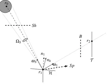
To take advantage of fast intersection calculations and parallel computing, we implement our MCM algorithm within the EDStar framework (De La Torre et al., 2014). We start with an algorithm refered as Monte Carlo Fixed Date, or MCFD. It is meant for the design of heliostat fields of Central Receiver Systems (CRS) considering a single date. It predicts the solar power P incident on the receiver. It is very similar to the first example presented at section 4.1 in ( De La Torre et al. (2014)): rays are sampled from the heliostat field and are followed until they reach or miss the central receiver. A Monte Carlo weight is associated to each sampled ray and P is evaluated as the average value of a large number of such weights. The details of the ray-sampling procedure are given hereafter. r1 r0 ωS ΩS nh n1 ω1 r2 T H Sh B Sp
Figure 1: Schematic representation of the Monte Carlo Fixed Date (MCFD) algorithm
(1) A location r1 is uniformly sampled on the reflective surface of the whole
(2) A direction ωS is uniformly sampled within the solar cone ΩS of angular
radius θS.
(3) An effective normal vector nh is sampled around the ideal normal vector
n1at r1representing reflection and pointing imperfections. ω1corresponds
to the specular reflection of −ωS by a surface normal to nh
(4) r0 is defined as the first intersection with a solid surface of the ray starting
at r1 in the direction ωS
(a) If r0belongs to an heliostat surfaceH or to the receiver T , a shadowing
effect appears and the Monte Carlo weight is ˆw = 0 ;
(b) If r0 doesn’t exist (or is at the sun), the location r2 is defined as the
first intersection with a solid surface of the ray starting at r1 in the
direction ω1
(i) If r2 belongs to something else than the receiver T , there is a
blocking effect and the Monte Carlo weight is ˆw = 0 ;
(ii) If r2 doesn’t exist there is a spillage effect and the Monte Carlo
weight is ˆw = 0 ;
(iii) If r2 belongs to the receiver T , the Monte Carlo weight is ˆw = DN I× ρ × (ωS· nh)× SH+
This algorithm is equivalent to the integral formulation of Eq. (1) (see Fig. 1). (1) P = ∫ DH+ pR1(r1) dr ∫ DΩS pΩS(ωS) dω ∫ DNh pNh(nh|ωS; b) dn ˆw
with the Monte Carlo weight :
ˆ w = H(r0∈ H ∪ T ) × 0 +H(r0∈ H ∪ T ) ×/ { H(r2∈ T ) × 0/ +H(r2∈ T ) × DNI × ρ × (ωS· nh)× SH+ } (2) and probability density functions :
(3) pR1 = 1 SH+ (4) pΩS = 1 ∫ ΩS dωS = 1 2π(1− cos θS) (5) pNh(nh|ωS; b) = ( 1 + 1 b ) × (nh· n1)1+ 1 b 2π× ( 1− cos2+1 b ( π 4 − 1 2 × arccos (ωS· n1) ))
As presented by De La Torre et al. (2014) in section 4.1, reflection and point-ing imperfections are modelled with the Blinn’s model (Pharr and Humphreys, 2010), of parameter b. This microfacet model consists in an overall angular spreading obtained by a distribution of effective normal vectors nh around the
ideal normal n1. This model introduces an exponential falloff to approximate
the distribution of microfacet normals1 and appears in the probability density
function pNh(nh|ωS; b).
2.2. Formulation of the lifetime-collected energy
Strong benefits are expected from the establishment of a rigorous equiva-lence between the algorithm and the integral formulation: a modification of one leads to a modification of the other and vise versa. This allows the choice of either working on the very intuitive nature of the photon-tracking algorithm, or on the mathematical features of the formulation (De La Torre et al., 2014). When modifying the algorithm directly, the formulation helps to check that the modification is rigorous. When working on the formulation, there is no question about rigor and the Monte Carlo algorithm is obtained by translating the suc-cessive integrals into sucsuc-cessive sampling events. This is the case here: instead of discretizing lifetime and performing a computation at each date, which would require a considerable amount of time, we simply modify Eq. (1), integrating it over time and introducing a probability density pτ, which leads to an algorithm
in which each ray-sampling is preceeded by the sampling of a date along lifetime. Eq. (1) becomes (6) E = ∫ Lifetime P (t)dt = ∫ Lifetime pτ(t) dt ∫ DH+ pR1(r1) dr ∫ DΩS(t) pΩS(t)(ωS(t)) dω ∫ DNh pNh(nh|ωS(t); b) dn ˆw(t)
with time-dependent probability density functions
(7) pΩS(t)= 1 ∫ ΩS(t) dωS(t) = 1 2π(1− cos θS(t)) (8) pNh(nh|ωS(t); b) = ( 1 +1 b ) × (nh· n1) 1+1 b 2π× ( 1− cos2+1 b ( π 4 − 1 2 × arccos (ωS(t)· n1) )) 1The distribution of n
his truncated to avoid the occurence of reflected directions towards
the surface for quasi-tangent incidences. Thus, the angular spreading is dependent on the incident direction ωS.
and the Monte Carlo weight that now is ˆ w(t) = H(r0∈ H ∪ T ) × 0 +H(r0∈ H ∪ T ) ×/ H(r2∈ T ) × 0/ +H(r2∈ T ) × DN I(t)× (ωS(t)· nh)× SH+ pτ(t) (9) In this formulation, time is continous but the climatic data that we used took the form of a succession of DNI values every hour. We therefore needed an interpolation assumption: as a first order approach we assumed that DNI was a one hour piecewise constant function of time. As far as the sampling probability
pτ(t) is concerned, we used an importance sampling approach: pτ(t) is simply
a normalised form of DNI,
(10)
pτ(t) =
DN I(t)
∫
Lifetime DN I(t) dt
This means that the dates with the larger DNI values are sampled more fre-quently than the low DNI ones. This introduces no biais because pτ(t) appears
both in the integral and in the weight. Practically speaking, this simply means that DNI data are pre-treated: only the non zero DNI values are kept, they are classified in ascending order, cumulated and normalised. Then, when we need to sample time according to pτ(t), a value of this cumulative function is
sam-pled uniformly in the unit interval and the corresponding one-hour time-interval is retained. Hereafter, the corresponding algorithm is refered as Monte Carlo Solar Tracker, or MCST. The ray-sampling procedure becomes:
(1) A DN I is uniformly sampled over the lifetime period according to pτ(t)and
the corresponding one-hour time-integral is retained
(2) A location r1 is uniformly sampled on the reflective surface of the whole
heliostat fieldH+ of surface S
H+
(3) A direction ωS is uniformly sampled within the solar cone ΩS of angular
radius θS.
(4) An effective normal vector nh is sampled around the ideal normal vector
n1at r1representing reflection and pointing imperfections. ω1corresponds
to the specular reflection of −ωS by a surface normal to nh
(5) r0 is defined as the first intersection with a solid surface of the ray starting
at r1 in the direction ωS
(a) If r0belongs to an heliostat surfaceH or to the receiver T , a shadowing
−6 −4 −2 0 2 4 6 Receiver size (m) −6 −4 −2 0 2 4 6 Receiver size (m) 0 400 800 1200 1600 2000 2400 2800 3200 3600 Flux density in kW m − 2
(a) Flux density map at PS10 receiver on
March 21st with DN I = 1000 W m−2 in kW m−2 −6 −4 −2 0 2 4 6 Receiver size (m) −6 −4 −2 0 2 4 6 Receiver size (m) 0 1500 3000 4500 6000 7500 9000 Energy density in MW h m − 2
(b) Energy density map at PS10 receiver
during a year in MW h m−2
Figure 2: Flux density and energy density maps
(b) If r0 doesn’t exist (or is at the sun), the location r2 is defined as the
first intersection with a solid surface of the ray starting at r1 in the
direction ω1
(i) If r2 belongs to something else than the receiver T , there is a
blocking effect and the Monte Carlo weight is ˆw = 0 ;
(ii) If r2 doesn’t exist there is a spillage effect and the Monte Carlo
weight is ˆw = 0 ;
(iii) If r2 belongs to the receiver T , the Monte Carlo weight is ˆw = DN I(t)× ρ × (ωS(t)· nh)× SH+
pτ(t)
3. Implementation
In order to test the performance of the MCST algorithm, as well as for validation purposes, it is run with the characteristics of a reference Central Re-ceiver System. PS10, a 11 MWe power plant, has been the subject of several
studies from which data are available. It is located near Seville, in Spain, and is the world’s first commercial concentrating solar power plant. Its heliostat field consists in 624 heliostats following a radial staggered layout (Siala and Elayeb, 2001). Each heliostat has a surface of 121 m2 and concentrates sun rays to a
receiver, located at the top of a 115 m high tower, that feeds a steam turbine. Each sun position is translated into a DNI value coming from Typical Meteo-rological Year (TMY) data that correspond to a typical year on the considered site. As we have no better information, when adressing a lifetime prediction, we make the assumption that the climate will be identical every year and the lifetime simulation becomes strictly identical to a yearly simulation. Therefore only yearly simulations will be presented. According to the design, this power
plant should annualy produce 23 GWhe(electrical energy) and about 95 GWhth
(thermal energy) (Osuna et al., 2006). With MCST algorithm we have estimated 97 GWhth. This result indicates a very good agreement with the litterature data
and we retain it as a first MCST-validation exercise. For internal validation, we also performed time discretization using a deterministic approach for shorter time-intervals. This required that a seperate Monte Carlo run was performed for each date with MCFD algorithm and that each Monte Carlo reached a high enough accuracy level so that we only tested the time-integration part of the algorithm. Adequation was perfect, which fully validated our statistical inte-gration procedure.
Table 1 presents a comparison of MCST (yearly integration) and MCFD algorithms in terms of computational times and number of required realizations for a relative standard deviation (%RSD) of 0.1%, where %RSD is defined as
(11) %RSD =σ
¯
x× 100
where σ is the standard deviation of Monte Carlo weights and ¯x is the average
of Monte Carlo weights.
MCFD algorithm performances are presented for March 21st at noon and
March 21st at 6PM. Figures [2a; 2b] display sun spots : one for March 21st
at noon and one on a yearly integrated basis. The main point is that time integration with MCST requires 26 times more realizations than MCFD for March 21st at 12PM but 11 times less realizations than MCFD for March 21st
at 6PM. This simply reflects the fact that these two particular dates are close to the extreme cases. For March 21st at noon, there is nearly no optical losses (blocking, shading and spillage phenomena) and the optical integration is quite simple. On the contrary, at 6PM, optical losses require an accurate optical integration which translates into more Monte Carlo realizations. In any case, this confirms that time integration is not the main source of statistical difficulty in the CSP-design context. We claimed in introduction that annual integration could be performed with computational time comparable to that of a single date simulation. This is not true when comparing with favorable dates but is even an understatement when we consider disavantageous dates. In appendix, the yearly simulation time of 28 s is reduced to 2.8 s thanks to further computer-graphics optimization.
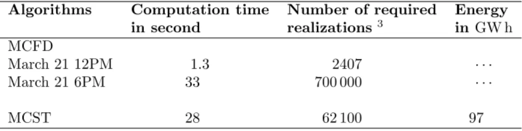
Table 1: Comparison of the computation time for Monte Carlo Fixed Date and Monte Carlo Sun Tracker algorithm for a relative standard deviation %RSD = 0.1%
Algorithms Computation time Number of required Energy in second realizations3 in GW h
MCFD
March 21 12PM 1.3 2407 · · ·
March 21 6PM 33 700 000 · · ·
4. Conclusion
Our main message is that statistical approaches make it possible to address lifetime integrated quantities with the same ease as temporal quantities. There is therefore no need to simplify the physical representation of the concentration process itself. We have illustrated this potential with the PS10 example, but up to now we have not entered into the details of what is now possible using this integration technique. The next step will be to consider phenomena such as :
• optical ageing of CSP components along lifetime extended up to fifty years
or longer
• accurate representation of climatic fluctuations (annual DNI change) • and even representation of predicted climate changes (long-term DNI change)
Acknowledgments
The authors acknowledge financial support from Total New Energies.
AppendixA. Optimization of the computation time
For optimization purposes, two ways are explored in order to reduce the MCST CPU time. To differentiate each code version, the following notation is introduced :
MCSTa the original algorithm (see 2.2)
MCSTb using the first optimization
MCSTc using the second optimization
AppendixA.1. First optimization
Considering that re-orientation (therefore at each date) of heliostats at each realization is time consuming, the aim is is here to reduce the number of sample dates. As it is necessary to preserve estimation accuracy, the idea is here to sample several rays per date. This is the concept of systematic sampling (Dunn and Shultis, 2011): Nr rays are sampled and followed onto the field for each
sampled date. The corresponding integral formulation is modified and Eq. (6) becomes Eq. (A.1) and MCSTa becomes MCSTbalgorithm.
(A.1) E = ∫ Lifetime pτ(t) dt Nr ∑ n=1 1 Nr ∫ DH+ pR1(r1) dr ∫ DΩS(t) pΩS(t)(ωS(t)) dω ∫ DNh pNh(nh|ωS(t); p) dn ˆw th
AppendixA.2. Second optimization
The second optimization has nothing to do with the Monte Carlo algorithm (the integral formulation) itself. The integral formulation remains the same as equation Eq(A.1). Here we optimize the photon tracking algorithm using computer graphics techniques. The sun tracking performed during MCST real-izations implies that the geometry of the solar installation is updated at each solar position. The re-positioning of the heliostat field and of the bounding boxes associated to each heliostat, for a sun position consists in performing ma-trix multiplications, each heliostat position being described with a 4× 4 matrix (Pharr and Humphreys (2010)). The computation time devoted to this step be-comes huge when simulating a large scale central receiver system with hundreds of heliostats. We developed heliostat-reorientation algorithm that reduces this computation time. Each heliostat is enclosed into an enlarged cubic bounding box. This bounding box includes all the positions that an heliostat can take when tracking the sun.
AppendixA.3. Results
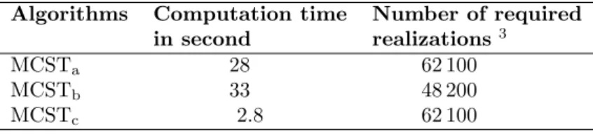
Table 2 displays the computation time associated to these two optimizations. The first optimization reduces the variance (the number of required realizations) but increases the computation time. It is therefore rejected. For the second opti-mization the number of realizations is strictly identical, the integral formulation is indeed inchanged but the computation time is reduced by approximately a factor ten2 for MCST algorithm.
Table 2: Comparison of the computation time of the several versions of Monte Carlo Sun Tracker algorithms for a relative standard deviation %RSD = 0.1%
Algorithms Computation time Number of required in second realizations3
MCSTa 28 62 100
MCSTb 33 48 200
MCSTc 2.8 62 100
References
P. Schwarzb¨ozl, R. Pitz-Paal, M. Schmitz, Visual HFLCAL - A software tool for layout and optimization of heliostat fields, in: Proceedings of 15th So-larPACES Conference, 1–8, 2009.
2The computation time is given for a desktop PC with AMD Phenom II X6 1055T 2.8 GHz
and 12 Go RAM.
P. Gilman, N. Blair, M. Mehos, C. Christensen, S. Janzou, C. Cameron, Solar advisor model user guide for version 2.0, National Renewable Energy Labo-ratory, 2008.
P. Garcia, A. Ferri`ere, J. J. B´ezian, Codes for solar flux calculation dedicated to central receiver system applications: A comparative review, Solar Energy 82 (3) (2008) 189–197.
M. Sanchez, M. Romero, Methodology for generation of heliostat field layout in central receiver systems based on yearly normalized energy surfaces, Solar Energy 80 (2006) 861–874.
F. Collado, Quick evaluation of the annual heliostatfield efficiency, Solar Energy 82 (2008) 379–384.
P. K. Falcone, A handbook for solar central receiver design, Tech. Rep., Sandia National Labs., Livermore, CA (USA), 1986.
J. De La Torre, G. Baud, J. B´ezian, S. Blanco, C. Caliot, J. Cornet, C. Coustet, J. Dauchet, M. El Hafi, V. Eymet, R. Fournier, J. Gautrais, O. Gourmel, D. Joseph, N. Meilhac, A. Pajot, M. Paulin, P. Perez, B. Piaud, M. Roger, J. Rolland, F. Veynandt, S. Weitz, Monte Carlo advances and concentrated solar applications, Solar Energy 103 (2014) 653–681.
M. Pharr, G. Humphreys, Physically Based Rendering, second edition : from theory to implementation, Morgan Kaufmann Publishers, 2010.
F. M. F. Siala, M. E. Elayeb, Mathematical formulation of a graphical method for a no-blocking heliostat field layout, Renewable energy 23 (1) (2001) 77–92. R. Osuna, R. Olavarr´ıa, R. Rafael Morillo, Construction of a 11MW Solar Ther-mal Tower Plant in Seville, Spain, in: Proceeding of 13 th Solar PACES Symposium, Seville, Spain, 2006.