HAL Id: hal-00938866
https://hal.inria.fr/hal-00938866
Submitted on 29 Jan 2014HAL is a multi-disciplinary open access archive for the deposit and dissemination of sci-entific research documents, whether they are pub-lished or not. The documents may come from teaching and research institutions in France or
L’archive ouverte pluridisciplinaire HAL, est destinée au dépôt et à la diffusion de documents scientifiques de niveau recherche, publiés ou non, émanant des établissements d’enseignement et de recherche français ou étrangers, des laboratoires
Systems Modelers
Albert Benveniste, Timothy Bourke, Benoît Caillaud, Bruno Pagano, Marc
Pouzet
To cite this version:
Albert Benveniste, Timothy Bourke, Benoît Caillaud, Bruno Pagano, Marc Pouzet. A Type-Based Analysis of Causality Loops In Hybrid Systems Modelers. 2013. �hal-00938866�
Investissements d’Avenir
Développement de l’Economie Numérique
"Briques génériques du logiciel embarqué"
Sys2soft
Trustable Embedded Software for Systems that are tightly coupled with
Physics
WP3.1
D3.1_1
A Type-Based Analysis of Causality Loops
In Hybrid Systems Modelers
Albert Benveniste (Inria)
Timothy Bourke (Inria)
Benoît Caillaud (Inria)
Bruno Pagano (Esterel Technologies)
Marc Pouzet (École Normale Supérieure)
Version du document: 1.0 Date: 20/01/2014
Historique du document
Version du
document Date Rédacteur (s) Commentaire / modifications
0.0 06/01/2014 Benoît Caillaud (Inria) Version initiale du livrable 1.0 24/01/2014 Benoît Caillaud (Inria) Première version du livrable
Contents
1 Synth`ese . . . 4
1.1 Identification du projet . . . 4
1.2 Objet du document . . . 4
1.3 Contraintes . . . 4
2 Causality and Scheduling Issues in Modelers . . . 5
3 A Core Synchronous Language with ODEs . . . 11
4 Non-standard Semantics and Standardization . . . 12
4.1 Non-Standard Semantics . . . 12
4.2 Standardization . . . 17
4.3 Key properties . . . 18
5 Two Type-based Causality Analyses . . . 19
5.1 A Lustre-like Causality Analysis . . . 19
5.2 A Schizophrenic Causality Analysis . . . 24
6 The Main Theorem . . . 27
6.1 A Nonsmooth Model . . . 27
6.2 Discussion . . . 28
7 Discussion and Related Work . . . 33
1
Synth`
ese
1.1
Identification du projet
Programme BGLE 2
Projet (Acronyme) Sys2soft
Date de commencement 1er juin 2012 Date d’ach`evement 30 novembre 2015
1.2
Objet du document
Une question centrale dans la conception des langages de mod´elisation des syst`emes hy-brides, y compris Modelica, est la d´etection, `a la compilation, des circuits alg´ebriques ou boucles de causalit´e. De tels circuits provoquent le blocage du mod`ele lors de sa simulation et empˆechent la g´en´eration de code ordonanc´e statiquement.
Ce livrable d´etaille une solution `a ce probl`eme, pour un langage de mod´elisation hybride qui combine des equations de flots `a la Lustre et des equations diff´erentielles ordinaires. Le langage comporte un op´erateur last(x) dont la valeur est la limite `a gauche de la variable x. Cet op´erateur permet de casser des circuits alg´ebriques et a l’avantage de s’appliquer indiff´eremment sur des variables discretes ou continues. La s´emantique du langage est `a base de nombres r´eels non-standards et d´efinit une ex´ecution comme une suite de pas, progressant de mani`ere infinit´esimale. Un signal est consid´er´e causalement correct quand il peut ˆetre calcul´e s´equentiellement et est continu en dehors des instants o`u un pas de calcul discret a lieu. L’analyse de causalit´e est d´efinie sous la forme d’un syst`eme d’inf´erence de type . Il est prouv´e que dans tout programme correctement typ´e, les signaux sont continus en dehors des seuls instants o`u des calculs discrets ont lieu. Cette analyse de causalit´e permet de g´en´erer un code de simulation ordonnanc´e statiquement qui fait appel `a une biblioth‘eque standard de solveurs de syst`emes d´equations differentielles.
La pertinance de cette approche est illustr´ee par plusieurs exemples ´ecrits dans le langage Z´elus, qui est un langage de mod´elisation des syst`emes hybrides, qui combine des equations de flˆots synchrones et des equations diff´erentielles.
1.3
Contraintes
2
Causality and Scheduling Issues in Modelers
Tools for modeling hybrid systems [8] such as Modelica,1 LabVIEW,2 and Simulink/
Stateflow,3 are now rightly understood and studied as programming languages. Indeed,
models are used not only for simulation, but also for test-case generation, formal verifica-tion and translaverifica-tion to embedded code. This explains the need for a formal operaverifica-tional semantics for specifying their implementations and proving them correct [18,10].
The underlying mathematical model is the synchronous parallel composition of Ordi-nary Differential Equations (ODEs) or Differential Algebraic Equations (DAEs), stream equations, hierarchical automata, and imperative features. While each of these features taken separately is precisely understood, real languages allow them to be combined in sophisticated ways. One major difficulty in modelers is the treatment of causality loops.
Causality or algebraic loops [22, 2-34] pose problems of well-definedness and compila-tion. They can lead to models that are mathematically unsound, and prevent simulators from statically ensuring the existence of a fixed point, and compilers from generating stat-ically scheduled code. The static detection of such loops, termed causality analysis, has been extensively studied and implemented since the mid-1980s in synchronous language compilers combining stream equations and control structures [13,14,15,6,1]. The classi-cal and simplest solution is to reject loops which do not cross a unit delay. For instance, the Lustre-like equations:4
x = 0 -> pre y and y = if c then x + 1 else x
define the two sequences (xn)n∈N and (yn)n∈N such that:
x(0) = 0 y(n) = if c(n) then x(n) + 1 else x(n)
x(n) = y(n − 1)
They are causally correct since the feedback loop for x contains a unit delay pre y (for “previous”). Replacing pre y with y would make the two equations non-causal. Causally correct equations can be statically scheduled to produce a sequential loop-free step function. Below is an excerpt of the C code generated by the Heptagon compiler [12] of Lustre:
if (self->v_1) {x = 0;} else {x = self->v_2;}; if (c) {y = x+1;} else {y = x;};
self->v_2 = y; self->v_1 = false;
It computes current values of x and y from that of c. The internal memory of function
step is in self, with self->v 1 initialized to true and set to false and self->v 2 storing
the value of pre y. 1 http://www.modelica.org 2 http://www.ni.com/labview 3 http://www.mathworks.com/products/simulink 4
The unit delay 0 -> pre(·), initialized to 0, is written 1
ODEs with resets Consider now the situation of a program defining continuous-time signals only, made of ODEs and equations.
der y = z init 4.0 and z = 10.0 - 0.1 * y and k = y + 1.0
defines signals y, z and k, where for all t 2 R+, dy
dt(t) = z(t), y(0) = 4.0, z(t) = 10.0 − 0.1 ·
y(t), and k(t) = y(t) + 1.5 This program is causal simply because it is possible to generate
a sequential function derivative(y) = let z = 10.0 − 0.1 ⇤ y in z and initial value 4.0 for y so that a numeric solver [9] can compute a sequence of approximations y(tn) for increasing
values of time tn 2 R+ and n 2 N. Thus, for continuous-time signals, integrators break
algebraic loops just as delays do for discrete-time signals.
Can we reuse the simple justification we used for data-flow equations? Consider the value that y would have if computed by an ideal solver taking an infinitesimal step of duration ∂ [5]. Writing ?y(n), ?z(n) and ?k(n) for the values of y, z and k at instant n∂,
with n 2?N a non-standard integer, we have
?y(0) = 4 ?z(n) = 10 − 0.1 ·?y(n)
?y(n + 1) =?y(n) +?z(n) · ∂ ?k(n) =?y(n) + 1
where ?y(n) is defined sequentially from past values and ?y(n) and ?y(n + 1) are
infinites-imally close, for all n 2 ?N, yielding a unique solution for y, z and k. The equations are
thus causally correct.
Troubles arise when ODEs interact with discrete-time constructs, for example when a reset occurs at every occurrence of an event. E.g., the sawtooth signal y : R+ 7! R+ such
that dydt(t) = 1 and y(t) = 0 if t 2 N can be defined by an ODE with reset,
der y = 1.0 init 0.0 reset up(y - 1.0) -> 0.0
where y is initialized with 0.0, has derivative 1.0, and is reset to 0.0 every time the zero-crossing up(y - 1.0) is true, that is, whenever y - 1.0 crosses 0.0 from negative to positive. Is this program causal? Again, consider the value y would have were it calculated by an ideal solver taking infinitesimal steps of length ∂. The value of ?y(n) at instant n∂,
for all n 2?Nwould be:
?y(0) = 0 ?y(n) = if?z(n) then 0.0 else?ly(n)
?ly(n) = ?y(n − 1) + ∂ ?c(n) = (?y(n) − 1) ≥ 0
?z(0) = false ?z(n) =?c(n) ^ ¬?c(n − 1)
This set of equations is clearly not causal: the value of ?y(n) depends instantaneously on ?z(n) which itself depends on ?y(n). There are two ways to break this cycle: (a) consider
that the effect of the zero-crossing is delayed by one cycle, that is, the test is made on
?z(n − 1) instead of on z(n), or, (b) distinguish the current value of?y(n) from the value it
5
dery = e init v0stands for y =
1
would have had were there no reset, namely ?ly(n). Testing a zero-crossing of ly (instead
of y),
?c(n) = (?ly(n) − 1) ≥ 0,
gives a program that is causal since ?y(n) no longer depends instantaneously on itself. We
propose writing this |6:
der y = 1.0 init 0.0 reset up(last y - 1.0) -> 0.0
where last(y) stands for ly, that is, the left-limit of y. In non-standard semantics [5], it is infinitely close to the previous value of y, and written ly(n) ⇡ y(n − 1). In the case where y is defined by its derivative, last(y) is the so-called “state port” of the integrator block
1
s of Simulink, which is introduced expressly to break causality loops like the one above
|.7 According to the Simulink documentation [21, 2-685]:
The output of the state port is the same as the output of the block’s standard output port except for the following case. If the block is reset in the current time step, the output of the state port is the value that would have appeared at the block’s standard output if the block had not been reset.
Simulink restricts the use of the state port. It is only defined for the integrator block and it cannot be returned as a block output: it may only be referred to in the same context as its integrator block and used to break algebraic loops. The use of the state port causes subtle bugs in the Simulink compiler. Consider the Simulink model given in Figure 1a
with the simulation results given by the tool for x and y in Figure1b. The model contains two integrators. The one at left, named ‘Integrator0’ and producing x, integrates the constant 1. The one at right, named ‘Integrator1’ and producing y, integrates x; its state port is fed back through a bias block to reset both integrators, and through a gain of −3 to provide a new value for Integrator0. The new value for Integrator1 comes from the state port of Integrator0 multiplied by a gain of −4. In our syntax|:
der x = 1.0 init 0.0 reset z -> -3.0 * last y and der y = x init 0.0 reset z -> -4.0 * last x and z = up(last x - 2.0)
Replaying the non-standard interpretation of signals, the equations above are perfectly causal: the current values of?x(n) and ?y(n) only depend on their previous values, that is:
?x(n) = if?z(n) then −3 ·?y(n − 1) else?x(n − 1) + ∂ ?y(n) = if?z(n) then −4 ·?x(n − 1)
else?y(n − 1) + ∂ ·?x(n − 1)
6
The |’s link to the web page: http://zelus.di.ens.fr/hscc2014/.
7
The Simulink integrator block outputs both an integrated signal and a state port. We write (x, lx ) =
1
s(x0, up(z), x
0) for the integral of x0, reset with value x0every time z crosses zero from negative to positive,
with output x and state port lx . The example would thus be written:
(y, ly) = 1
?x(0) = 0 ?y(0) = 0
?c(n) = (?x(n − 1) − 2) ≥ 0 ?z(n) =?c(n) ∧ ¬?c(n − 1)
Yet, can you guess the behavior of the model and explain why the trajectories computed by Simulink are wrong?
Initially, both x and y are 0. At time t = 2, the state port of Integrator1 becomes equal to 2 triggering resets at each integrator as the output of block u − 2.0 crosses zero. The results show that Integrator0 is reset to −6 (= 2 · −3) and that Integrator1 is reset to 24 (= −6 · −4). The latter result is surprising since, at this instant, the state port of Integrator0 should also be equal to 2, and we would thus expect Integrator1 to be reset to −8 (= 2 · −4)! Scope Integrator1 1 s xo Integrator0 1 s xo Gain1 −4 Gain0 −3 Constant 1 Bias u−2.0 x y
(a) Simulink model
-6 -4 -2 0 2 0 0.5 1 1.5 2 2.5 3 x 0 5 10 15 20 25 0 0.5 1 1.5 2 2.5 3 Time y (b) Simulation results
Fig. 1: A miscompiled Simulink model (release R2009b) ♣
The Simulink implementation does not satisfy its documented behavior [21, 2-685]. Inspecting the C function which computes the current outputs, mdlOutput in Figure2, the code of the two integrators appears in an incorrectly scheduled sequence. At the instant of
the zero-crossing (conditions ssIsMajorTimeStep(S) and zcEvent are true), the state port of Integrator0 (stored in sGetContStates(S) -> Integrator0 CSTATE) is reset using the state port value of Integrator1. Thus, Integrator1 does not read the value of Integrator0’s state port (that is ?x(n − 1)) but rather the current value (?x(n)) leading to an incorrect output. The Simulink model is not correctly compiled — it needs another variable to store the value of ?x(n − 1), just as a third variable is normally needed to swap the values
of two others. We argue that such a program should either be scheduled correctly or give rise to a warning or error message.
Any loop in Simulink, whether of discrete- or continuous-time signals, can be broken by inserting the so-called memory block [21, 2-831].8 If x is a signal, mem(x) is a piecewise
constant signal which refers to the value of x at the previous integration step (or major step). If those steps are taken at increasing instants ti ∈ R, mem(x)(t0) = x0 where
t0 = 0 and x0 is an explicitly defined initial value, mem(x)(ti) = x(ti−1) for i > 0 and
mem(x)(ti+ δ) = x(ti−1) for 0 δ < ti+1− ti. As integration is performed globally, mem(y)
may cause strange behaviors as the previous value of a continuously changing signal x depends precisely on when the solver decides to stop! | Writing mem(y) is thus unsafe in general [4].9 There is nonetheless a situation where the use of the memory block is
mandatory and still safe:
The program only refers to the previous integration step during a discrete step. This situation is very common: it is typically that of a system with continuous modes M1
and M2 producing a signal x, with each of them being started with the value computed
previously by the solver, and mem(x) being used to pass a value from one mode to the other |. Instead of the unsafe operator mem(x), we better need to refer to the left limit of x, and write it again last(x). Yet, the unrestricted use of this operation may cause a new kind of causality loop which have to be statically rejected. Consider the following equation activated at a continuous time base:
y = -1.0 * (last y) and init y = 1.0
which defines, for all n 2?N, the sequence ?y(n) such that: ?y(n) = −?y(n − 1) ?y(0) = 1
Indeed, there is little difference with an equation y = -1.0 * y. Even though ?y(n) can
be computed sequentially, its value does not increase infinitesimally at each step, that is, y is not left continuous while no signal is looked for a zero-crossing. For any time t 2 R, the set {n∂ | n 2 ?N^ n∂ ⇡ t ^?y(n) 6⇡ ?y(n + 1)} is infinite. Thus, the value of y(t) at any standard instant t 2 R is undefined.
8
In contrast, the application of a unit delay 1
z to a continuous-time signal is statically detected and
results in a warning.
9
Quoting the Simulink manual (http://www.mathworks.com/help/simulink/slref/memory.html), “Avoid using the Memory block when both these conditions are true: - Your model uses the variable-step solver ode15s or ode113. - The input to the block changes during simulation.”
// P_0 = -2.0 P_1 = -3.0 P_2 = -4.0 P_3 = 1.0 static void mdlOutputs(SimStruct * S, int_T tid) { _rtX = (ssGetContStates(S)); ... _rtB = (_ssGetBlockIO(S)); _rtB->B_0_0_0 = _rtX->Integrator1_CSTATE + _rtP->P_0; _rtB->B_0_1_0 = _rtP->P_1 * _rtX->Integrator1_CSTATE; if (ssIsMajorTimeStep (S)) { ... if (zcEvent || ...) { (ssGetContStates (S))->Integrator0_CSTATE = _ssGetBlockIO (S))->B_0_1_0; } ... } (_ssGetBlockIO (S))->B_0_2_0 = (ssGetContStates (S))->Integrator0_CSTATE; _rtB->B_0_3_0 = _rtP->P_2 * _rtX->Integrator0_CSTATE; if (ssIsMajorTimeStep (S)) { ... if (zcEvent || ...) { (ssGetContStates (S))-> Integrator1_CSTATE = (ssGetBlockIO (S))->B_0_3_0; } ... } ... }
Fig. 2: Excerpt of C code produced by RTW (release R2009b)
Contribution and Organization of the Paper This paper presents the causality problem for a core language that combines Lustre-like stream equations, ODEs with reset and a basic control structure. The operator last(x) stands for the previous value of x in non standard semantics and coincide with its left-limit when x is left-continuous. This operation plays the role of a delay but is safer than the memory block mem(x) as its semantics does not depend on any particular solver. When x is a continuous-state variable, it coincides with the so-called Simulink state port. We develop a non-standard semantics following [5] and a compile-time causality analysis in order to detect possible instantaneous loops. The static analysis takes the form of a type system, reminiscent of the simple Hindley-Milner type system for core ML [23]. A type signature for a function expresses the instantaneous dependences between its inputs and outputs. We prove that well typed programs only progress by infinitely small steps outside of zero-crossing events, that is,
signals are continuous during integration. We are not aware of such a correctness theorem based on static typing for hybrid modelers.
The presented material has been implemented in Z´elus, [7] a synchronous Lustre-like language extended with ODEs. Moreover, all examples in the paper are written with Z´elus.
The paper is organized as follows. Section 3 introduces a core synchronous language with ODEs. Section 4 presents its semantics based on non-standard analysis. Section 5
presents two type systems for causality and Section 6 a major property: any well-typed program is proved not to have any discontinuities during integration. Section 7 discusses related work and we conclude in Section 8.
3
A Core Synchronous Language with ODEs
We now introduce a kernel language. It is not intended to be a full language but a minimal one for the purpose of the present paper. It allows for writing data-flow equations, ordinary differential equations and control structures. The syntax is given below.
d ::= let x = e | let k f (p) = e where E | d; d
e ::= x | v | op(e) | e fby e | last(x) | f (e) | (e, e) | up(e) p ::= (p, p) | x
E::= () | x = e | init x = e | next x = e | der x = e | E and E | local x in E | if e then E else E | present e then E else E
k ::= D | C | A
A program is a sequence of definitions (d), of either a value (let x = e) that binds the value of expression e to x, or a function (let k f (p) = e where E). In a function definition, k is the kind of the function f , p denotes formal parameters, and the result is the value of an expression e which may contain variables defined in the auxiliary equations E. There are three kinds of function: k = A means that f is a combinational function (typically a function imported from the host language, e.g., addition); k = D means that f is a sequential function that must be activated at discrete instants (typically a Lustre function with an internal discrete state); k = C denotes a hybrid function that may contain ODEs and which must be activated continuously. An expression e can be a variable (x), an immediate value (v), e.g., a boolean, integer or floating point value, the point-wise application of an imported function (op(e)) such as +, ⇤ or not(·), an initialized delay (e1fby e2), the left-limit of
a signal (last(x)), a function application (f (e)), a pair (e, e) or a rising zero-crossing detection (up(e)), which, in this language kernel, is the only basic construct to produce an event from a continuous-time signal (e). A pattern p is a tree structure of identifiers (x). A set of equations E is either an empty equation (()); an equality stating that a pattern
equals the value of an expression at every instant (x = e); the initialization of a state variable x with a value e (init x = e); the value of a state variable x at the next instant (next x = e); or, the current value of the derivative of x (der x = e). An equation can also be the conjunction of two sets of equations (E1 and E2); the declaration that a variable
x is defined within, and local to, a set of equations (local x in E); a conditional that activates a branch according to the value of a boolean expression (if e then E1else E2),
and a variant that operates on an event expression (present e then E1 else E2).
Notational abbreviations:
(a) if e then E def= if e then E else ().
(b) present e then E def= present e then E else (). (c) der x = e init e0
def
= init x = e0 and der x = e
(d) der x = e init e0 reset z ! e1 def
=
init x= e0 and present z then x= e1 else der x = e
Equations (E) must be in Static Single Assignment (SSA) form, that is, every variable has a unique definition at every instant.
4
Non-standard Semantics and Standardization
4.1
Non-Standard Semantics
Let ?R and ?N be the non-standard extensions of R and N. ?N is totally ordered and
every set that is bounded from above (resp. below) has a unique maximal (resp. minimal) element. Let ∂ 2 ?R be an infinitesimal, i.e., ∂ > 0, ∂ ⇡ 0. Let the global time base or
base clock be the infinite set of instants:
T@ = {tn = n∂ | n 2?N}
T@ inherits its total order from ?N; in addition, for every element of R+ there exists an infinitesimally close element of T@. Whenever possible we leave ∂ implicit and write T
instead of T@. Let T = {t0n | n 2 ?N} ✓ T. T (i) stands for t0i, the i-th element of T . In
the sequel, we only consider subsets of the time base T obtained by sampling a time base on a boolean condition or a zero-crossing event. Any element of a time base will thus be of the form k∂ where k 2 ?N. If T ✓ T, we write •T(t) the immediate predecessor of t in
T and T•(t) the immediate successor of t in T . For an instant t, we write its immediate
predecessor and successor as, respectively, •t and t•, rather than as •T(t) and T•(t). For
t 2 T ✓ T, neither •t nor t• necessarily belong to T . min(T ) is the minimal element
of T and t T t0 means that t is a predecessor of t0 in T . The clock of a signal x is
Definition 1 (Signals): Let V⊥ = V + {?} where V is a set. S (V ) = T 7! V⊥ is the set of
signals. A signal x : T 7! V⊥ is a total function from a time base T ✓ T to V⊥. Moreover,
for all t 62 T, x(t) = ?. If T is a time base, x(T (n)) and x(tn) are the value of x at instant
tn where n 2?N is the n-th element of T .
Sampling: Let bool = {false, true} and x : T 7! bool⊥. The sampling of T according
to x, written T on x, is the subset of instants defined by:
T on x= {t | (t 2 T ) ^ x(t) = true} Note that as T on x ✓ T , it is also totally ordered. Let x : T 7! ?R
⊥. The zero-crossing
of an x is up(x) : T 7! bool⊥. To underline the fact that up(x) is defined only when
t2 T, we write up(x)(T )(t) for its value at time t. Outside of T , up(x)(T )(t) = ?. In the definition below, < is the total order on ?R.
up(x)(T )(t0) = false where t0 = min(T )
up(x)(T )(t) = 9n 2?N, n≥1. ^ (x(t−n∂) < 0) ^(x(t−(n−1)∂) = 0) ^ . . . ^(x(t−∂) = 0) ^(x(t) > 0) (1) where t 2 T
The above definition means that a zero-crossing on x occurs when x goes from a strictly negative to a strictly positive value, possibly with intermediate values equal to 0.
Let V be a set of values closed under product and sum. ?V is its non-standard extension
such that?(V
1⇥ V2) =?V1⇥?V2,?V = V for any finite set V . ?V⊥=?V +{?} with ? as the
minimum element. Let L = {x1, ..., xn, ...} be a set of local variables and Lg = {f1, ..., fn, ...}
a set of global variables. An environment associates names to values. A local environment ρ and a global environment G map names to signals and signal functions:
ρ: L 7! S (?V) G: Lg 7!(S (?V) 7! S (?V))
Operations on environments: Consider ρ1 and ρ2.
• (ρ1+ ρ2)(x)(t) is ρ1(x)(t) if ρ2(x)(t) = ?, ρ2(x)(t) if ρ1(x)(t) = ?, and ? otherwise.
• ρ = merge (T ) (s) (ρ1) (ρ2) is the merge of two environments according to a signal
s 2 S (bool). The value of a signal x at instant t 2 T is the one given by ρ1 if
s(t) is true and that of ρ2 otherwise. Nonetheless, in case x is not defined in ρ1
(respectively ρ2), it implicitly keeps its previous value, that is ρ1(•clock (x)(t)). This
corresponds to adding an equation x = last(x) when no equation is given in one branch of a conditional. For all x and instant t 2 T , ρ(x)(t) = ρ1(x)(t) if s(t) = true
and x 2 Dom(ρ1); ρ(x)(t) = ρ(x)(•clock (x)(t)) if s(t) = true and x 62 Dom(ρ1).
ρ(x)(t) = ρ2(x)(t) if s(t) = false and x 2 Dom(ρ2); ρ(x)(t) = ρ(x)(•clock (x)(t))
?[[e]]⇢ G(T )(t) = ?, ? if t 62 T ?[[v]]⇢ G(T )(t) = v, false ?[[x]]⇢ G(T )(t) = ρ(x)(t), false ?[[op(e)]]⇢ G(T )(t) = let v, z =?[[e]] ⇢ G(T )(t) in op(v), z ?[[(e 1, e2)]]⇢G(T )(t) = let v1, z1 =?[[e1]]⇢G(T )(t) in letv2, z2=?[[e2]]⇢G(T )(t) in (v1, v2), (z1_ z2) ?[[e
1fbye2]]⇢G(T )(t0) = ?[[e1]]⇢G(T )(t0) if t0 = min(T ) ?[[e
1fbye2]]⇢G(T )(t) = ?[[e2]]⇢G(T )(•T (t)) otherwise ?[[last(x)]]⇢ G(T )(t) = ρ(x)(•clock(x)(t)), false ?[[f (e)]]⇢ G(T )(t) = let s(t0), z(t0) =?[[e]] ⇢ G(T )(t0) in letv0, z0 = G(f )(s)(t) in v0, z(t) _ z0 ?[[up(e)]]⇢ G(T )(t) = let s(t0), z(t0) =?[[e]] ⇢ G(T )(t0) in letv0 = up(s)(T )(t) in v0, z(t) _ v0
Fig. 3: The Non-standard Semantics of Expressions
Expressions: Expressions are interpreted as signals and node definitions as functions from signals to signals. For expressions, we define ?[[e]]⇢
G(T )(t) such that for every instant t 2 T ,
it returns both the value of e and a Boolean value true if e raises a zero-crossing event. The definition is given in Figure3.
Let us explain the definition. The value of expression e is considered undefined outside of T . The current value of an immediate constant v is v and no zero-crossing event is raised. The current value of x is the one stored in the environment ρ(x) and no event is raised. The semantics of op(e) is obtained by applying the operation op to e at every instant, an event is raised only if e raises one. An expression (e1, e2) returns a pair at every instant
and raises an event if either of e1 or e2 raises one. The initial value of a delay e1fby e2 is
that of e1. Afterward, it is the previous value of e2 according to clock T . E.g., the value of
0 fby x on clock T is the value x had at the previous instant that T was active. This is not necessarily the previous value of x. On the contrary, last(x) is the previous value of x, the last time x was defined. The semantics of f (e) is the application of the function f to the signal value of e, which raises an event when either e or the body of f raises one. Finally, the semantics of up(e) is given by operator up(.), which raises a zero-crossing event when
?[[x = e]]⇢
G(T ) = [s/x], z where 8t 2 T.s(t), z(t) =?[[e]] ⇢ G(T )(t) ?[[E
1 andE2]]⇢G(T ) = ρ1+ ρ2, z1or z2 where ρ1, z1=?[[E1]]⇢G(T ) ^ ρ2, z2 =?[[E2]]⇢G(T ) ?[[present e then E
1 elseE2]]⇢G(T ) =
ρ0, z or z
1or z2 where 8t 2 T.s(t), z(t) =?[[e]]⇢G(T )(t)
and ρ1, z1=?[[E1]]⇢G(T on s)
and ρ2, z2=?[[E2]]⇢G(T on not(s))
and ρ0= merge (T ) (s) (ρ 1) (ρ2) ?[[if e then E 1elseE2]]⇢G(T ) = ρ0, z or z 1or z2 where 8t 2 T.s(t), z(t) =?[[e]]⇢G(T )(t) and ρ1, z1=?[[E1]]⇢G(T on s)
and ρ2, z2=?[[E2]]⇢G(T on not(s))
and ρ0= merge (T ) (s) (ρ 1) (ρ2) ?[[init x = e]]⇢ G(T ) = [s/x], z where s(t0), z(t0) =?[[e]] ⇢ G(T )(t0) and t0 = min(T ) and 8t 6= t0.s(t) = ρ(x)(t) ^ z(t) = false ?[[next x = e]]⇢ G(T ) = [s/x], z where 8t 2 T. (v, z =?[[e]] ⇢ G(T )(t)) ^ (s(t•) = v) ?[[der x = e]]⇢ G(T ) = [s/x], z where 8t 2 T. (v, z =?[[e]] ⇢ G(T )(t)) ^ (s(t•) = s(t) + ∂ ⇥ v)
Fig. 4: The Non-standard Semantics for Equations either e raises one or up(s)(T )(t) is true.
Equations: If E is an equation, G is a global environment, ρ is a local environment and T is a time base, ?[[E]]⇢
G(T ) = ρ0, z means that the evaluation of E on the time base T
returns a local environment ρ0 and a zero-crossing signal z. As for expressions, the value
of E is undefined outside of T , that is, for all t 62 T , ρ0(x)(t) = ? and z(t) = ?. For all
t 2 T , z(t) = true signals a zero-crossing occurs at instant t and z(t) = false means that no zero-crossing occurred at that instant. The semantics of equations is given in Figure4, where the following notation is used: If z1 : T 7! bool? and z2 : T 7! bool?then
z1 or z2 : T 7! bool? and 8t 2 T.(z1 or z2)(t) = z1(t) _ z2(t) if z1(t) 6= ? and z2(t) 6= ?,
Function definitions: Function definition is our final concern: we must show the existence of fixed points in the sense of Kahn process network semantics based on Scott domains.
The prefix order on signals S (V ) indexed by T is defined as: signal x is a prefix of signal y, written x S(V )y, if x(t) 6= y(t) implies x(t0) = ? for all t0 such that t t0. The
minimum element is the undefined signal ?S(V ) for which 8t 2 T, ?S(V )(t) = ?. When
possible, we write ? for ?S(V ) and x y for x S(V ) y. The symbolWdenotes a supremum
in the prefix order. A function f : S (?V ) 7! S (?V ) is continuous if Wif (xi) = f (
W
ixi)
for every increasing chain of signals, where increasing refers to the prefix order. If f is continuous, then equation x = f (x) has a least solution denoted by fix (f ), and equal to W
ifi(?). We name such continuity on the prefix order Kahn continuity [16].
The prefix order is lifted to environments so that ρ ρ0 iff for all x 2 Dom(ρ)[Dom(ρ0),
ρ(x) ρ0(x). It is lifted to pairs such that (x, y) (x0, y0) iff x x0 and y y0.
Property 1 (Kahn continuity): Let [s/p] be an environment, G a global environment of Kahn-continuous functions and T a clock. The function:
F : (L 7! S (?V )) ⇥ S (bool) 7! (L 7! S (?V )) ⇥ S (bool) such that:
F (ρ, z) = let ρ0, z0 =?[[E]]⇢+[s/p]
G (T ) in ρ0, z or z0
is Kahn continuous, that is, for any sequence (ρi, zi)i≥0:
F (Wi∈I(ρi, zi)) =Wi∈I(F (ρi, zi))
Proof: We only provide a sketch. We first need to prove the result for expressions listed in Figure 3. We only review the expressions involving the non-standard semantics in a nontrivial way, as the other cases are routine. Consider e1fbye2 and last(x). None of
these expressions contributes to the second (zero-crossing) field of the semantics, so only the first field matters. In fact, the Kahn continuity of e1fbye2 is proved exactly as for
Lustre [3], since only the total ordering of the underlying time index matters and the argument lifts without change from N to T. The same holds for last(x), which corresponds to pre(x) in Lustre in the lifting from N to T. The expression up(e) contributes to the second field of the semantics. Formula (1) defining up(x) is causal and thereby Kahn continuous. We then consider the equations of Figure 4. We discuss only next x = e and derx = e since the other cases as handled as in Lustre (including the composition of equations E1 and E2). Consider the first field of the semantics. If e returns the value v
at the considered instant t, then the first field of x returns v at the next instant t•, i.e.,
x(t•) = v(t). Kahn continuity follows directly. The same reasoning holds for der x = e. ⇤
As a consequence, an equation (ρ, z) = F (ρ, z) admits a least fixed point fix (F ) = W
i(Fi(?, ?)).
The declaration of ?[[let k f (p) = e where E]]
G(T ) defines a Kahn-continuous function ?f such that
?
where ?f (T )(s)(t) = let s0(t0), z(t0) = ?[[e]]⇢0+[s/p] G (T )(t0) in s0(t), z(t) _ z0(t) and with (ρ0, z0) = fix ((ρ, z) 7!? [[E]]⇢+[s/p]G (T ))
Yet, Kahn-continuity of?f does not mean that the function computes anything interesting.
In particular, the semantics gives a unique meaning to functions that become ‘stuck’, like10
let hybrid f(x) = y where rec y = y + x
The semantics of f is ?f (x) = ? since the minimal solution of equation y = y + x is ?.
The purpose of the causality analysis is to statically reject this kind of program.
4.2
Standardization
We now relate the non-standard semantics to the usual super-dense semantics of hybrid systems. Following [20], the execution of a hybrid system alternates between integration steps and discrete steps. Signals are now interpreted as total functions from the time index S= R⇥N to V
?. This time index is called super-dense time [20,18] and is ordered lexically,
(t, n) <S(t0, n0) iff t <Rt0, or t = t0 and n <Nn0. Moreover, for any (t, n) and (t, n0) where
n N n0, if x(t, n0) 6= ? then x(t, n) 6= ?.
A timeline for a signal x is a function Nx : R+ 7! N?. Nx(t) is the number of instants
of x that occur at a real date t and such timelines thus specify a subset of super-dense time SN
x = {(t, n) 2 S | n NNx(t)}. In particular, if Nx is always 0, then SNx is isomorphic to
R+. For t 2 R and T ✓ T, define:
set(T )(t)def= {t0 2T | t0 ⇡t ^ t 2 R} ✓ T
that is, the set of all instants infinitely close to t. T is totally ordered and hence so is
set(T )(t). Let x : T 7!?V
?.
We now proceed to the definition of the timeline Nx of x and the standardization of x,
written
st(x) : R ⇥ N 7! V?, such that st(x)(t, n) = ? for n > Nx(t).
Let T0 def= set(T )(t) and consider
st(x(T0))def= {st(x(t0)) | t0 2T0}.
(a) If st(x(T0)) = {v} then, at instant t, x’s timeline is N
x(t) = 0 and its standardization
is st(x)(t, 0) = v. 10
(b) If st(x(T0)) is not a singleton set, then let
Z def= {t0 | t0 2T0^x(t0) 6⇡ x(T0•(t0))}
i.e., Z collects the instants at which x experiences a non-infinitesimal change. Z is either finite or infinite:
(i) If Z = {tz0, . . . , tzm} is finite, timeline Nx(t) = m and the standard value of
signal x at time t is:
8n 2 {0, . . . , m}.st(x)(t, n) = st(x(tzn))
(ii) If Z is infinite (it may even lack a minimum element), let Nx(t) = ? and 8n.st(x)(t, n) = ?
which corresponds to a Zeno behavior.
Our approach differs slightly from [18], where the value of a signal is frozen for n > N (t). We decide instead to set it to the value ?. Each approach has its merits. For ours, parts of signals that do not experience jumps are simply indexed by (t, 0) which we identify with t. In turn, we squander the undefined value ? which is usually devoted to Scott-Kahn semantics and causality issues.
4.3
Key properties
We now define two main properties that reasonable programs should satisfy. The first one states that discontinuities do not occur outside of zero-crossing events, that is, signals are continuous during integration. The second one states that the semantics should not depend on the choice of the infinitesimal. These two invariants are sufficient conditions to ensure that a standardization exists.
Invariant 1 (All discontinuities aligned on zero-crossings): An expression e evaluated under G, ρ and a base time T has no discontinuity outside of zero-crossing events. Formally, define s(t), z(t) =?[[e]]⇢
G(T )(t), then 8t, t0 2T such that t t0:
t ⇡ t0 )(9t00 2T, t t00 t0 ^ z(t00)) _ s(t) ⇡ s(t0)
This invariant states that signals must evolve continuously during integration. Discrete changes must be announced to the solver using the construct up(.). Not all programs satisfy the invariant, e.g.,
f takes a single argument () of type unit and returns a value y. Writing ?y(n) for the value of y at instant n∂ with n 2 ?N, we get ?y(0) = 0 and ?y(n) = ?y(n − 1) + 1. Yet, ?y(n) 6⇡?y(n − 1) while no zero-crossing is registered for any instant n 2?N. This program
will be statically rejected by using the type system developed in the next section.
Invariant 2 (Independence from ∂): The semantics of e evaluated under G, ρ and a base time T is independent of the infinitesimal time step. Formally, define s(t) = fst(?[[e]]⇢
G(T@)(t))
and s0(t) = fst(?[[e]]⇢
G(T@0)(t)), then:
8t 2 R, n 2 N, st(s)(t, n) = st(s0)(t, n)
When satisfied, this invariant ensures that properties and values on non-standard time carry over to standard time and values.
5
Two Type-based Causality Analyses
Programs are statically typed. We adopt, for our language, the type system presented in [4]. Well-typed programs may still exhibit causality issues, that is, the definition of a signal at instant t may instantaneously depend on itself. We present two systems. The first essentially amounts to checking that every loop is broken either by a unit delay or an integrator. It is reminiscent of the causality analysis of both Lustre and Lucid Synchrone. Yet, the operation last(x) can only be activated at a discrete instant. The second is more expressive and exploits the fact that last(x) is the left limit of a signal allowing to analyze the Simulink example of Section 2. It thus breaks causality loops during discrete steps but not during integration steps.
The analysis aims to give sufficient conditions for the invariants1 and2. We adopt the convention quoted below [4,5]. A signal is termed discrete if it only changes on a discrete
clock :
A clock is termed discrete if it has been declared so or if it is the result of a zero-crossing or a sub-sampling of a discrete clock. Otherwise, it is termed
continuous.
A discrete change on x at instant t 2 T means that x(•t) 6⇡ x(t) or x(t) 6⇡ x(t•). Said
differently, all discontinuities have to be announced using the programming construct up(.).
5.1
A Lustre-like Causality Analysis
A classical causality analysis is to reject loops which do not cross a delay. This ensures that outputs can be computed sequentially from current inputs and an internal state. This simple solution is used in the academic Lustre compiler [13], Lucid Synchrone [24] and Scade 6.11 We propose generalizing it to a language mixing stream equations, ODEs
and their synchronous composition. 11
Two classes of approaches exist to formalize causality analyses. In the first class, the causality is defined as an abstract preorder relation on signal names. The causality preorder evolves dynamically at each reaction. The considered program is causally correct if its associated causality preorder is provably a partial order at every reaction. In the second class, the causality is defined as the tagging of each event by a ”stamp” taken from some preordered set. The considered program is causally correct if its set of stamps can be partially ordered—somehow like Lamport vector clocks. Previous works [1, 5] belong to the first class, whereas this paper belongs to the second class.
Our analysis associates a type to every expression and function via two predicates:
(typ-exp) states that, under constraints C, global environment G, local environment H, and kind k 2 {A, D, C}, an expression e has type ct;(typ-env)states that under constraints C, global environment G, local environment H, and kind k, the equation E produces the type environment H0.
(typ-exp)
C | G, H `k e : ct
(typ-env)
C | G, H `k E : H0
The type language is
σ ::= 8α1, ..., αn: C. ct !k ct ct ::= ct ⇥ ct | α
k ::= D | C | A
where σ defines type schemes, α1, ..., αn are type variables and C is a set of constraints.
A type is either a pair (ct ⇥ ct) or a type variable (α). The typing rules for causality are defined with respect to an environment of causality types. G is a global environment mapping each function name to a type scheme (σ). H is a local environment mapping each variable x to its type ct:
G ::= [σ1/f1, ..., σk/fk] H ::= [ct1/x1, ..., ctn/xn]
If H1 and H2 are environments, H1 + H2 is their disjoint union. H1, H2 is their
concate-nation; and H1 ⇤H2 is a new environment such that (H1 + [x : ct]) ⇤ (H2 + [x : ct]) =
(H1⇤H2) + [x : ct] where + and ⇤ are associative and commutative.
Precedence relation: C is a precedence relation between variables with the following intuition. If C | G, H `k e : α1 holds and α1 < α2, the current value of e is ready at time
α1 then it is also ready at a later instant α2. < must be a strict partial order: it must not be possible to deduce α < α from the transitive closure of C.
C ::= {α1 < α01, ..., αn< α0n}
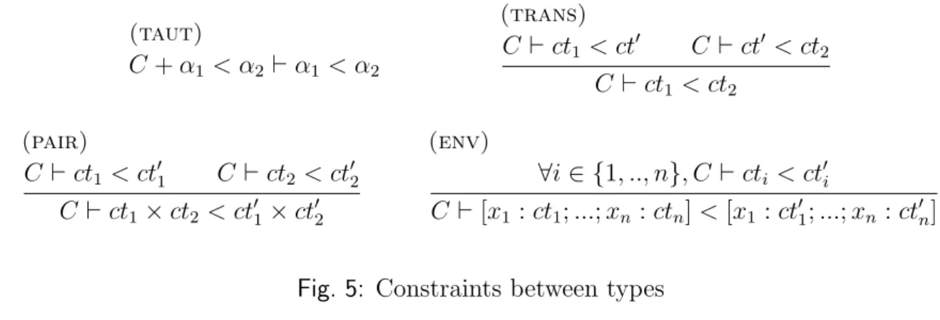
The predicate C ` ct1 < ct2, defined in Figure 5, means that ct1 precedes ct2 according to
(taut) C + ↵1 < ↵2 ` ↵1 < ↵2 (trans) C ` ct1 < ct0 C ` ct0 < ct2 C ` ct1 < ct2 (pair) C ` ct1 < ct01 C ` ct2 < ct02 C ` ct1⇥ct2 < ct01⇥ct02 (env) 8i 2 {1, .., n}, C ` cti < ct0i C ` [x1 : ct1; ...; xn: ctn] < [x1 : ct01; ...; xn : ct0n]
Fig. 5: Constraints between types
The initial environment G0 gives type signatures to imported operators, synchronous
primitives and the zero-crossing function.
(+), (−), (⇤), (/) : 8↵. ↵ ⇥ ↵! ↵A pre(·) : 8↵1, ↵2 : {↵2 < ↵1}. ↵1 D ! ↵2 · fby · : 8↵1, ↵2 : {↵1 < ↵2}. ↵1⇥ ↵2 D ! ↵1 up(·) : 8↵1, ↵2 : {↵2 < ↵1}. ↵1 C ! ↵2
For example, the operation x + y depends on both x and y, that is, it must be computed after x and y have been computed. Indeed, if C | G, H ` x : ↵1 and C | G, H ` y : ↵2,
C ` ↵1 < ↵ and C ` ↵2 < ↵, then C | G, H ` x + y : ↵. pre(x) does not depend on x.
Moreover, pre(x) has to be used before x is computed. For up(x), we consider in this first system that the effect of a zero-crossing is delayed by one cycle. Hence, up(x) does not depend instantaneously on x.
Instantiation/Generalization The types of global definitions are generalized to types schemes (σ) by quantifying over free variables.
genC(ct1 k
!ct2) = 8↵1, ..., ↵n : C.ct1 k
!ct2
where {↵1, ..., ↵n} = Vars(C) [ Vars(ct1) [ Vars(ct2). The variables in a type scheme σ
can be instantiated. ct 2 Inst(σ) means that ct is an instance of σ. For ~↵0 and k k0:
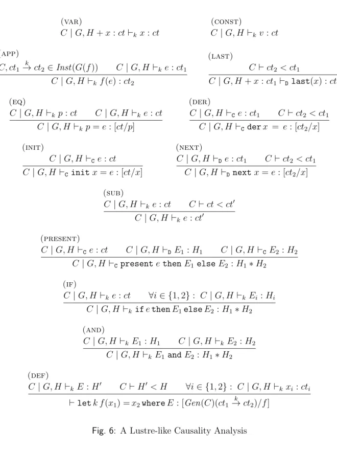
C[ ~↵0/~↵], ct1[ ~↵0/~↵]!k0 ct2[ ~↵0/~↵] 2 Inst(8~↵: C.ty1 !k ty2) The typing relation is defined in Figure 6 and described below. Rule (var). A variable x inherits the declared causality type ct. Rule (const). A constant v has any causality type.
(var) C | G, H + x : ct `k x : ct (const) C | G, H `k v : ct (app) C, ct1 k !ct2 2Inst(G(f )) C | G, H `k e : ct1 C | G, H `kf (e) : ct2 (last) C ` ct2 < ct1 C | G, H + x : ct1 `D last(x) : ct2 (eq) C | G, H `k p : ct C | G, H `k e : ct C | G, H `k p = e : [ct/p] (der) C | G, H `C e : ct1 C ` ct2 < ct1 C | G, H `C derx = e : [ct2/x] (init) C | G, H `C e : ct C | G, H `C initx = e : [ct/x] (next) C | G, H `D e : ct1 C ` ct2 < ct1 C | G, H `D nextx = e : [ct2/x] (sub) C | G, H `k e : ct C ` ct < ct0 C | G, H `ke : ct0 (present) C | G, H `C e : ct C | G, H `D E1 : H1 C | G, H `C E2 : H2
C | G, H `C presente then E1 elseE2 : H1⇤H2
(if) C | G, H `ke : ct 8i 2 {1, 2} : C | G, H `k Ei : Hi C | G, H `kife then E1elseE2 : H1⇤H2 (and) C | G, H `k E1 : H1 C | G, H `k E2 : H2 C | G, H `kE1 andE2 : H1⇤H2 (def) C | G, H `kE : H0 C ` H0 < H 8i 2 {1, 2} : C | G, H `kxi : cti
` letk f (x1) = x2whereE : [Gen(C)(ct1 k
!ct2)/f ]
Rule (app). An application f (e) has causality type ct2 if f has function type ct1 k
! ct2,
from the instantiation of a type scheme giving a new set of constraints C, and e has type ct1.
Rule (last). last(x) is the previous value of x. In this system, we only allow last(x) to appear during a discrete step (of kind D).
Rule (eq). An equation p = e defines an environment [ct/p] if p and e are of type ct. Rule (sub). If e is of type ct and ct < ct0 then e can also be given the type ct0.
Rule (der). An integrator has a similar role as a unit delay: it breaks dependencies dur-ing integration. If e : ct1 then any use of x does not depend instantaneously on the
computation of e and can thus be given a type ct2 such that ct2 < ct1.
Rule (present). The present statement returns an environment H1⇤H2. The first handler
is activated during discrete steps and the second one has kind C.
Rule (if). This rule is the same as that of the present statement except that the handlers and condition must all be of kind k.
Rule (def). For a function f with parameter x1 and result x2, the body E is first typed
under an environment H and constraints C. The resulting environment H0 must be
strictly less than H. This forbids any direct use of variables in H when typing E. We can now illustrate the system on several examples.
Example The following program is a classic synchronous (thus discrete-time) program. Calling the forward Euler integrator integr below, the function heat is valid since temp does not depend instantaneously on gain - temp. step is a global constant.
let node integr(xi, x’) = x where
rec x = xi -> pre x + (pre x’ * step) let node heat(temp0, gain) = temp where rec temp = integr(temp0, gain - temp))
The causality signatures are:
val integr : ’a * ’b -C-> ’a val heat : ’a * ’b -C-> ’a
The signature for integr states that the output depends instantaneously on its first argu-ment but not the second one. The following program is statically rejected:
Indeed, taken x : ↵x and y : ↵y, the first equation is correct if both C ` ↵x < ↵y and
C ` ↵y < ↵x. This means that C must contain {↵x < ↵y, ↵y < ↵x} which is cyclic. This
one is correct:
let hybrid f(x) = o where
rec der y = 1.0 - x init 0.0 and o = y + 1.0 let hybrid loop(x) = y where rec y = f(y) + x val f : {’b < ’a }.’a -C-> ’b
val loop : ’a -C-> ’a
Yet, the type system is that of a synchronous language and the restriction of last(x) to appear only in a discrete context is quite restrictive. We do now a little better.
5.2
A Schizophrenic Causality Analysis
To properly analyse what the causality rules should be when relaxing the use of last(x), let us turn to the non-standard semantics. In non-standard semantics, last(x) is the previous value of x.
last(x)(t) = x(•t)
When x is left-continuous, it coincides with the left limit since last(x)(t) ≈ x(t). Other-wise, it is the previously computed value of x. This means, in particular, that if a sequence of zero-crossings appears consecutively, termed a zero-crossing cascade, the current value of last(x) may change at every instant. Should we consider that last(x) breaks a causality cycle on x when x is continuous? No, since the equation x = last(x) + 1 with x initialized to 0 has no standard part. Thus, last(x) only breaks an algebraic loop during a discrete step, that is, when x may not be left-continuous. This is intuitive operationally if we con-sider the way simulation is performed in a hybrid modeler. A modeler alternates discrete steps (where side effects and state changes can occur) and integration steps. Consider a boolean variable d, true during discrete steps and otherwise false. The implementation of last(x) is simply:
last(x) = if d then pre(x) else x
During a discrete step, last(x) is a discrete register, otherwise it is the identify function. The dependence information associated to last(x) is thus conditional. The principle is to associate a pair ct1 + ct2 to every expression e such that (a) during discrete steps, e
only depends on ct1, and, (b) during integration steps, e only depends on ct2 . The type
language is modified accordingly.
σ ::= ∀↵1, ..., ↵n: C. ct → ct ct ::= ct × ct | ↵ + ↵ | ↵
where σ defines type schemes, ↵1, ..., ↵n are type variables and C is a set of constraints. A
type is either a pair (ct × ct), a compound of two type variables (↵ + ↵) or a type variable (↵).
The operation ↵1+ ↵2 is lifted to types. We consider the equality of types modulo the
following equation:
(ct1×ct2) + (ct01×ct20) = (ct1+ ct01) × (ct2+ ct02)
The typing rules for causality are also defined for typing environments. The structure of G and H is preserved and constraints are extended to account for types ct1 + ct2 in a
straightforward manner.
(sum)
C ` ct1 < ct01 C ` ct2 < ct02
C ` ct1+ ct2 < ct01+ ct02
Similarly, instantiation and generalization are unchanged. But we replace the rule (last)
of the system in Figure 6 with this one:
(last)
C ` ct0 1 < ct1
C, H + [x : ct1+ ct2] ` last(x) : ct01+ ct2
That is, last(x) does not depend on x during a discrete step, but it does during a contin-uous step.
Example last(x) does not necessarily break causality loops:
let hybrid g(x) = o where rec der y = 1.0 init 0.0
and z = last z + y and init z = 0.0
If z : ↵z+ βz and y : ↵y + βy, then last(z) : ↵0z+ βz. We also have: last(z) + y : ↵y + β
with βy, βz < β. There is a causality cycle since βy, βz < β 6< βz. This program is also
rejected:
let hybrid f(z) = y where
der y = 1.0 init -1.0 reset up(z) -> -1.0 let hybrid loop() = y where rec y = f(y)
Indeed, f takes the type signature 8↵1, ↵2 : {↵3 < ↵2}.(↵1+ ↵2) ! ↵1 + ↵3. The body of
loop is then typed. Let y : ↵y+ βy. Thus the function application f (y) is given the type
↵y + β0
y. The equation y = f (y) is well typed if ↵y + βy0 < ↵y + βy, that is, ↵y < ↵y and
β0
What should the signature of a zero-crossing be? As we discussed in Section2, numeric solvers can monitor certain signals for zero-crossings during integration. These signals need not be continuous. Nonetheless, classical methods for zero-crossing detection such as the ‘Illinois’ method [9] are both faster and more accurate for continuous signals. We can split up(·) into two operations according to the value of d:
up(x) = if d then upd(x) else upc(x)
up(x) is the disjoint union of two event detections and the two events cannot happen at the same time:
(a) upc(x) detects zero-crossings during integration. It is directly managed outside of the program by the numeric solver.
(b) upd(x) detects a zero-crossing when x has a discontinuity.
The implementation of upd(x) can be programmed in a synchronous manner. It is false at the very first instant and true when x goes from negative to positive while the current time (represented by a global signal t) does not change:
upd(x) = false -> (last(t) = t) ^ (last(x) ≤ 0) ∧ (x > 0) The signature for zero-crossing detection is thus:
upc(·) : ∀↵1, ↵2 : {↵2 < ↵1}.↵1 → ↵2
upd(·) : ∀↵1, ↵2, ↵3 : {↵3 < ↵2}.(↵1+ ↵2) → (↵1+ ↵3)
As a consequence, up(last(x)) does not depend on x.
Example If up(x) instantaneously depends on x during discrete time, then:
let hybrid f(x) returns o where
rec der y = 1.0 - x init 0.0 reset up(x) -> x and o = y + 1.0
let hybrid loop() returns y where rec y = f(last y) init 0.0
f gets the following signature:
Avoiding unbounded cascades of discrete zero-crossings By distinguishing the detec-tion of zero-crossings at discrete transidetec-tions from their detecdetec-tion during integradetec-tion, it is possible to identify unbounded cascades of discrete zero-crossings. This situation occurs when a discrete transition fires a new discrete transition for the next instant, and so on. Consider replacing the signature of upd(·) by:
upd(·) : 8↵. ↵ + ↵ ! ↵ + ↵ The following equation is now rejected:
der x = 1.0 init -1.0 reset upd(last x) -> -1.0
Indeed, x : ↵1+ ↵2, thus last(x) : ↵3+ ↵2, thus upd(last(x)) : ↵4+ ↵4 with ↵2, ↵3 < ↵4.
As ↵4 < ↵1 but ↵4 6< ↵2, the equation is invalid. Replacing upd(·) by upc(·) gives a valid
equation:
der x = 1.0 init -1.0 reset upc(last x) -> -1.0
Indeed: x : ↵1+ ↵2, thus last(x) : ↵3 + ↵2, thus upc(last(x)) : ↵4+ ↵5. As ↵4 < ↵1 and
↵5 < ↵2, the program is valid.
The new signature for upd(·) means that it is no longer considered to break feedback loops as would a zero-crossing performed during integration. Consequently, defining up(x) as the disjunction of upd(x) and upc(x) means that it cannot break loops either, and that it is a potential source of unbounded discrete cascades.
6
The Main Theorem
We can now state the main result of this paper. Well-typed programs have a standardiza-tion, that is, all signals are continuous during integration. This theorem requires assump-tions on primitive operators and imported funcassump-tions, as the following example shows.
6.1
A Nonsmooth Model
A detailed presentation of this example can be found online ♣. In a nutshell, it consists of several modules. The first two are an integrator and a time base with a parameterized initial value t0:
let hybrid integrator(y0, x) = y where rec init y = y0 and der y = x
let hybrid time(t0) = integrator(t0, 1.0)
Then a function producing a quasi-Dirac (Dirac with width > 0). It yields a function dirac(d, t) such that R−∞+∞dirac(d, t)dt = 1 for every constant d > 0.
let dirac(d, t) = 1 / pi * d / (d * d + t * t)
Our goal is to produce, using a hybrid program, an infinitesimal value for d, so that dirac(d, t) standardizes as a Dirac measure centered on t = 0. This can be achieved by integrating a pulse of magnitude 1, but of infinitesimal width. Such a pulse can be produced using a variable that is reset twice by the successive occurrences, separated by a ∂, of two zero-crossings:
let hybrid doublecrossing(t) = (x + 1.0) / 2.0 where rec init x = -1.0
and present up(t) then next x = 1.0 else
present up(x) then next x = -1.0 else der x = 0.0 let hybrid infinitesimal(t1,t) =
integrator(0.0, doublecrossing(t1))
The first zero-crossing in doublecrossing occurs when t crosses zero and causes an immediate reset of x from −1 to +1, this in turn triggers an immediate zero-crossing on x and a reset of x back to −1. The input of the integrator is thus one for one ∂-step; the output of the integrator, initially 0, becomes ∂ at time t1+ ∂.
The main program is the following, where t0 < t1 < t2:
let hybrid nonsmooth(t0, t1, t2) = x where rec t = time(t0)
and d = infinitesimal(t - t1)
and x = integrator(0.0, dirac(d,(t - t2)))
What is the point of this example? It is causally correct and yet its standardization has a discontinuity at t2 though no zero-crossing occurs. This is because dirac standardizes
to a Dirac mass.
6.2
Discussion
In the previous example, the problem arises with the function dirac. Indeed, d2+td 2 is not
defined when t = 0 and d = 0. However, it is defined everywhere when d6=0. In particular, it is defined for d = ∂ > 0. The solution seems clear: if a standard function f (x) of
a real variable x is such that f (x0) = ?, then our non-standard semantics must enforce
f (x) = ? for any x ⇡ x0. Applying this to the function d 7! d2d+t2 where t = 0 is fixed
gives @
@2+t2 = ?. This precludes the possibility of generating a Dirac mass as above. This
trick is formalized through the assumptions on operators and functions given below. Given x, y 2 ?R
, relation x ⇡ y holds iff st(x − y) = 0. Recall that function f :?R
7!
?R
is microcontinuous iff for all x, y 2?R
,
x ⇡ y implies f (x) ⇡ f (y). (2)
Recall that the microcontinuity of f implies the uniform continuity of st(f ):R7!R [19]. Denote [t0, t1]T= {t 2 T|t0 t t1}, with t0, t1 2 T finite.
Assumption 1: Operators op(·) of kind C are standard and satisfy the following definedness, finiteness and continuity properties:
8
<
:
op(?) = ?
8v, op(v) 6= ? implies op(v) finite
8u, v, u ⇡ v and op(u) 6⇡ op(v) implies op(u) = ?
Assumption 2: Environment G is assumed to satisfy the following assumption, for all ex-ternal functions f of kind C: for any bounded interval K = [t1, t2]T, for any input u that is
defined, finite and microcontinuous on K, if function G(f )(u) is defined and produces no zero-crossing in K, then it is assumed to be finite and microcontinuous on K:
" 8t 2 K, ( fst(G(f )(u)(t)) 6= ? and snd (G(f )(u)(t)) = false # + 2 4
8t 2 K, fst(G(f)(u)(t)) finite, and 8t, t0 2 K, t ⇡ t0implies
fst(G(f )(u)(t)) ⇡ fst(G(f)(u)(t0))
3
5
Assumption 1has several implications on the definitions of the usual operators. • For the square root function: p✏ = p−✏ = p0, for any ✏ ⇡ 0, which yields two
meaningful solutions: p✏= ? or p✏= 0
• For the inverse: 1/✏ = ? for any infinitesimal ✏ is the only solution.
• Consequently, the function sgn(x) = x/px2 returning the sign of x must satisfy
sgn(✏) = sgn(−✏) = sgn(0) = ?, for any infinitesimal ✏.
Theorem 1: Under Assumptions 1 and 2, every causally correct equation E (wrt. typing rules of Sections5.1 or5.2) satisfies Invariants 1 and 2and is standardizable.
This theorem is a direct consequence of the following lemmas:
Lemma 1: Assume that Assumptions 1 and 2 hold. For any activation clock T ✓ T,
for any bounded interval K = [t1, t2]T, for any environment ⇢ that is defined, finite and
microcontinuous on K, if expression e, of kind A or C, is defined and produces no zero-crossing on K, then it is finite and microcontinuous on K:
" 8t 2 K, ( fst(?[[e]]⇢ G(T )(t)) 6= ? and snd (?[[e]]⇢ G(T )(t)) = false # + 2 4 8t 2 K, fst(?[[e]]⇢ G(T )(t)) finite, and 8t, t0 2 K, t ⇡ t0implies fst(?[[e]]⇢ G(T )(t)) ⇡ fst( ?[[e]]⇢ G(T )(t0)) 3 5
Proof: Since?[[e]]⇢
G(T )(t) = ?, ? for all t 62 T , we can assume that K ✓ T . The Lemma is
proved by induction on the structure of expression e. We prove that it holds for all atomic expressions:
• The semantics of constant v, is a constant function ?[[v]]⇢
G(T )(t) = v, false. Thus it
is finite and microcontinuous.
• The semantics of expression x is a function of time defined in environment ρ:
?
[[x]]⇢G(T )(t) = ρ(x)(t), false
Which is by assumption defined, finite and microcontinuous on K. • ?[[last(x)]]⇢
G(T )(t): Two case must be distinguished, depending on the typing rules
used to assert the causal correctness of the expression. If the Lustre-like causality analysis applies (Section 5.1), then last(x) expressions are of kind D which is ruled out by assumption. Assume the Schizophrenic causality analysis applies (Section5.2). Recall no zero-crossing occurs on K. Hence:
?
[[last(x)]]⇢G(T )(t) ≈ ?
[[x]]⇢G(T )(t) = ρ(x)(t), false
Which is by assumption a defined, finite and microcontinuous function everywhere on K.
Then, we assume that the Lemma holds for all causally correct expressions e, e1 and e2 of
kind A or C, and prove that it holds for expressions built from e, e1 and e2, using one of
the following constructors: • ?[[(e
1, e2)]]⇢G(T )(t) is finite and microcontinuous if and only if ?[[(e
i)]]⇢G(T )(t), i = 1, 2
are defined and microcontinuous.
• Consider the application of operator op on expression e. Two cases must be distin-guished: First case, op is of kind D, in which case expression op(e) has the same kind, which is ruled out by assumption. Second case, op is of kind A. By Assumption 1, if defined, the semantics of op is a finite and microcontinuous function. Using the induction hypothesis,?[[op(e)]]⇢
G(T )(t) = op(v), z where v, z = ?[[e]]⇢
G(T )(t) is also finite
and microcontinuous.
• e1fbye2 expressions have kind D. Thus they can only appear in expression of the
same kind.
• In A or C expressions of the form f(e), f and e can not be of the kind D. Therefore Assumption2applies to function f and the induction hypothesis applies to expression e. Assume?[[f (e)]]⇢
G(T )(t) = v0, z(t)∨z0, where v0, z0 = G(f )(s)(t) and ∀t0.s(t0), z(t0) = ?[[e]]⇢
G(T )(t0) is defined and produces no zero-crossing in K. It is then the composition
of two finite and microcontinuous functions. It is, therefore, microcontinuous over K.
• ?[[up(e)]]⇢G(T )(t) defined and produces no zero crossing for all t 2 K implies that it is
constant and therefore microcontinuous over K.
Which proves that the induction hypothesis holds for all causally correct expression of kind
A or C. ⇤
Given a bounded interval T = [t0, t1]T, define the following nonstandard dynamical
system on T :
⇢
x(t0) = x0 finite
8t 2 T \ {t1}, x(t + ∂) = x(t) + ∂ ⇥ f(t, x(t))
Lemma 2: If the solution x : T 7! ?R of the dynamical system defined above is infinite or
discontinuous at t, then there exists t0 < t such that f (t0, x(t0)) is infinite.
Proof: We will be using the following property, for any t1 < t2: 9t02T , t 1t0t2, such that |x(t 0+@)−x(t0)| @ ≥ |x(t2)−x(t1)| t2−t1 . (3)
First case: Assume x(t) is infinite, for some t 2 T . Recall x(t0) is finite. Applying (3)
with t1 = t0, t2 = t yields the existence of t0, t0t0t such that |f(t0, x(t0))| ≥ |x(t)−x(t
0)|
t−t0 is
infinite.
Second case: Assume x(t) is not continuous for some t 2 T . There exists a t0 2 T ,
t0 ⇡ t, such that x(t0) 6⇡ x(t). Assume wlog that t0 < t. Observe that |x(t)−x(t0)|
t−t0 is infinite
since x(t) 6⇡ x(t0) and t ⇡ t0. Applying (3) with t
1 = t0, t2 = t yields the existence of
t00, t0t00t such that |f(t00, x(t00))| is also infinite. ⇤
The corollary of this lemma, is that under Assumptions 1 and 2, the semantics of equation der x = e is smooth provided that expression e is defined and triggers no zero-crossing:
Corollary 1: Assume that Assumptions1and2hold, and that e is a causally correct expres-sion of kind A or C. For any activation clock T ✓ T, for any bounded interval K = [t1, t2]T,
for any environment ρ that is defined, finite and microcontinuous on K, if the least fixed point of the operator ρ0, z0 7!?[[der x = e]]⇢0+⇢
G (T ) is defined and raises no zero-crossing on
K, then ρ0 is microcontinuous on K.
Proof: Assume ρ0 defined and z0 false on K. Assume ρ0 is infinite or discontinuous at
t 2 K. Using Lemma 2, there exists t0 2 K, t0 < t where the semantics of expression e, ?[[e]]⇢0+⇢
G (T )(t0) is infinite, which contradicts Lemma 1. ⇤
Lemma 3: Assume that Assumptions 1 and 2 hold. For any activation clock T ✓ T, for any bounded interval K = [t1, t2]T, for any environment ρ that is defined, finite and
microcontinuous on K, if the semantics of E, a causally correct equation of kind C, is defined and produces no zero-crossing on K, then it is finite and microcontinuous on K:
" 8x, 8t 2 K,( fst( ?[[E]]⇢ G(T ))(x)(t) 6= ? and snd (?[[E]]⇢ G(T ))(t) = false # ⇓ 2 4 8x, (8t 2 K, fst(?[[E]]⇢ G(T ))(x)(t) finite, and 8t, t0 2K, t ⇡ t0implies fst(?[[E]]⇢ G(T ))(x)(t) ⇡ fst( ?[[E]]⇢ G(T ))(x)(t0)) 3 5
Proof: By induction on the structure of equation E.
• Consider a causally correct equation of kind C and of the form x = e. The finiteness and microcontinuity of fst(?[[x = e]]⇢
G(T )) = fst( ?[[e]]⇢
G(T )) is a direct consequence of
Lemma 1.
• Equations init x = e and next x = e can not be typed with the sort C. Hence these cases are ruled out.
• Consider a causally correct equation of kind C and of the form der x = e. That
fst(?[[der x = e]]⇢
G(T )) is finite and microcontinuous is a direct consequence of
Corol-lary1.
We now proceed with compositions of equations. Assume that the lemma is valid for equa-tions E1and E2. We shall prove that it holds for equations E1 andE2, present e then E1 elseE2
and if e then E1elseE2:
• Consider a causally correct equation E = E1 and E2 of kind C. Finiteness and
microcontinuity of fst(?[[E]]⇢ G(T )) = fst(?[[E1]] ⇢ G(T )) + fst(?[[E2]] ⇢ G(T )) is a consequence
of the induction hypothesis.
• Consider equation E = present e then E1 else E2 and assume it to be causally
correct. Since snd (?[[E]]⇢
G(T )) is equal to false at every t 2 K, fst(?[[E]] ⇢
G(T )) =
fst(?[[E
2]]⇢G(T )) is finite and microcontinuous by induction hypothesis.
• Consider a causally correct equation E = if e then E1elseE2 of kind C. Type
correctness implies that expression e is a causally correct expression with the same kind. By Lemma 1, it is microcontinuous on K, and since its values are boolean, it is constant. Wlog, assume the expression evaluates to true. Hence, fst(?[[E]]⇢
G(T )) =
fst(?[[E
1]]⇢G(T )) is finite and microcontinuous by induction hypothesis.