HAL Id: hal-01187731
https://hal-mines-paristech.archives-ouvertes.fr/hal-01187731
Submitted on 27 Aug 2015HAL is a multi-disciplinary open access archive for the deposit and dissemination of sci-entific research documents, whether they are pub-lished or not. The documents may come from teaching and research institutions in France or abroad, or from public or private research centers.
L’archive ouverte pluridisciplinaire HAL, est destinée au dépôt et à la diffusion de documents scientifiques de niveau recherche, publiés ou non, émanant des établissements d’enseignement et de recherche français ou étrangers, des laboratoires publics ou privés.
Geostatistical Evaluation of Rock-Quality Designation
and its link with Linear Fracture Frequency
Serge Antoine Séguret, Cristian Guajardo Moreno
To cite this version:
Serge Antoine Séguret, Cristian Guajardo Moreno. Geostatistical Evaluation of Rock-Quality Desig-nation and its link with Linear Fracture Frequency. IAMG 2015, InterDesig-national Association of Math-ematical Geosciences, Sep 2015, Freiberg, Germany. �hal-01187731�
Geostatistical Evaluation of Rock-Quality Designation and its link with
Linear Fracture Frequency
S. A. SEGURET1* and C. GUAJARDO2
1Geosciences/Geostatistics – Mines ParisTech, France, serge.seguret@mines-ParisTech.fr 2
Geotechnique - Codelco, Chile *presenting author
1 Introduction
For mining operations in the developed world, staff safety has become a major concern where knowledge, at different scales, of the rock-mass strength is required in order to adequately size the retaining walls and other underground infrastructures, or simply the benches and face slopes in open-pit mining.
One of the identified causes of fragility is fracturation. By fracturation we mean discontinuities visible on core samples, including “open” fractures or just “joints”.
Fracturation can be tested in the laboratory on samples, providing attributes such as the Point Load Test (PLT, Bieniawski 1975); or measured on core samples, such as the two attributes of interest in this paper: the Rock-Quality Designation (Deere & Al., 1967; Stagg & Zienkiesicz, 1968) and the (Linear) Fracture Frequency (Jaeger & Cook, 1969).
RQD relates to measurements of intact lengths, FF to the counting of discontinuities, and these two quantities are related: when FF increases, RQD tends to decrease, but in a non-deterministic manner as shown by many studies (Priest & Hudson 1981, Sen & Kazi 1984).
The objective of this paper is to study this relation, together with one of the features common to both measurements: their directionality. By directionality, we simply mean that the measurement depends on the direction of the survey i.e. that these quantities are the components of a tensor, a feature rarely, if ever, considered in practice.
If the directionality of FF can be forgotten by correcting this measurement for an angular bias
(Terzaghi, 1965), such an operation is not possible with RQD, and we show that correcting FF but not RQD involves a distortion of their correlations, leading to increased influence of FF to the detriment of RQD in the Rock-Mass Rating, which is a comprehensive index of rock-mass quality used for the design and construction of rock excavations (Barton & Al., 1974). This creates a dilemma: either FF is corrected, inducing the described problems, or FF is not corrected and one must account for the sample direction during the estimation of FF at a grid nodes, the ultimate goal of this work. A third way is proposed: referring to a theoretical model linking FF and RQD, and using this reference to correct RQD. The chosen model is due to Priest & Hudson (1976). Although it is based on a
questionable assumption, it has been widely studied in the literature and proved to correctly reflect the link between the two attributes (Wallis & King 1980; Goodman & Smith 1980).
In the following, we do not address the thorny problem of making measurements made along lines representative of a volume.
2 Rock-Quality Designation (RQD)
2.1 Definition
The aim of RQD is to measure the degree of jointing or fracturing in a rock mass. It measures the borehole core recovery percentage incorporating only pieces of solid core that are longer than 100 mm measured along the centerline of the core. Figure 1 shows an example. Notice that joints along the core axis are treated as solid core. For mapping RQD, one has to consider samples of the same length (the case in the following application).
Figure 1. Detail of RQD calculation. Property highlighted in red is a cause of directionality
2.2 Directionality
RQD depends on the angle between the sample direction and the fracture; the primary reason is that a core with a joint running along it is considered solid (Figure 1, in red circles). If the sample direction is slightly changed, the joint is no longer aligned with the sample and a core, previously considered as longer than 10 cm and incorporated into RQD, can be rejected, which changes the final value of the attribute.
The second reason is that the spacings between the fractures are subject to directional bias. Suppose that all the fractures are parallel planes aligned along a single direction (Figure 2a) and consider two consecutive fractures (Figure 2b).
Figure 2. RQD directionality, detail of the calculations
The spacing measured along direction n°1 is l1 while it should be
l
1sin
if we want to make the measurement independent of the sample direction by referring to direction n°2 perpendicular to the fracture direction (similar to the Terzaghi correction presented later). This correction must be applied to each segment (Figure 2c) but it cannot be applied directly to their sum with the common factorsin( )
because after correction some segments may be shorter than 10 cm (case of segment l2 inFigure 2c) and consequently, they will not be included in the summation. The problem becomes more complex when we consider that a direction in three dimensions requires two angles (azimuth and dip) while, in practice, only the angle between the fracture and the sample is roughly evaluated on the samples.
If we assume that all the samples have the same direction, and the fracture network is isotropic (Figure 3a), the directionality of RQD can be neglected, whereas if there are local anisotropies in the fracture network, the local value of RQD at location “x” will depend on their angles and will not be comparable to another value of RQD at an another location “x’” even close to “x” (Figure 3b). In the first case RQD measures the degree of fracturation in an objective way but, in the second case it also measures the anisotropy of the fracture network and this is not really its objective.
Figure 3. a) Not considering the RQD directionality implicitly supposes that the fracture network is isotropic. b) In case of anisotropy, RQD depends on the sample direction.
2.3 Additivity & Estimation procedure
It results from the previous discussion that to map RQD, one must account for the sample direction. Now if we assume all the sample directions to be identical, this attribute is additive. To prove this, take two values known along two different supports L1 and L2, each with their own sum of core pieces longer than 10 cm, respectively equal to L10cm, 1 and L10cm, 2 .
The value of RQD associated with the support L1 L is: 2
1 2 10 , 1 10 , 2 1 2
100
cm cm L L L L RQDL
L
10 , 1 10 , 2 1 2 1 2 1 2100
L cm100
L cmL
L
L
L
L
L
1 2 1 2 1 2 L L RQD RQDL
L
L
L
This is, by definition, the way to combine additive quantities, equal to the average when L1=L2. So kriging RQD is authorized, at punctual or block scale, using classical geostatistical tools when RQD is order-two stationary.
If the calculation is easy, the interpretation is not: as RQD is a 1D measurement, estimating it at block scale using 1D samples just gives the average behavior of 1D samples over a block, and this is not a 3D property.
The samples have different directions and to make possible an interpretation of the estimation result, the samples must first be classed according to their directions, and structural analyses must be conducted by direction. If the variograms by sample directions are close to each other, and close to the variogram obtained with all the samples, there is no reason to distinguish between the directions because the fracture network looks isotropic. If this is not the case, kriging must be conducted only with the samples of a given directional sampling class, giving as many directional results as there are classes. If, for each location x, where the estimation is conducted, the results are always similar, it means that the directionality of the measurement can be neglected and kriging can be conducted with all the samples without distinction between the classes. If the differences are large, the result is directional, which is important for the geotechnicians because it means that, when looking at the rock-strength to drill a tunnel, for example, they must account for the drilling direction. This situation is discussed later in the application section.
3 Linear Fracture Frequency (FF)
3.1 Definition
The (Linear) Fracture Frequency is basically the ratio of a number of fractures, counted by the geologist, divided by the sample length. But the calculation is not simple because a significant part of the sample may be crushed, making the fracture counting possible only on the non crushed part. FF then becomes the ratio of two quantities both of which change from one location to another in the ore
deposit. It is not additive and needs some care when estimated by kriging (Seguret & al., 2014). In the following and for the application, the samples used have no crushed parts.
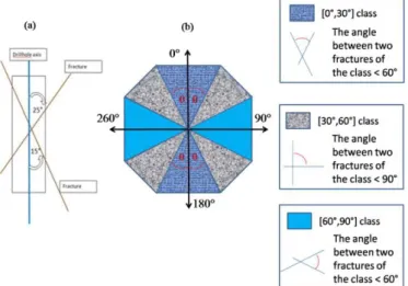
For each fracture, the geologist evaluates its angle with the sample axis without considering the fracture plane, and the fracture is classed into one of the three angular classes: [0°, 30°], [30°, 60°], [60°, 90°]. Normally, a direction in 3D is defined by the vector of the azimuth and the dip, but the only measurement at our disposal is θ, the angle between the sample axis and the fracture. In Fig. 4a, both fractures belong to the same [0, 30°] set because no orientation is given to the sample axis and the smaller angle is taken.
Figure 4. The angular classification is crude. a) Both fractures belong to the same set. c) In the middle class (grey), two fractures can be perpendicular
The possible directions included in each class are cones represented by a cross-section in Fig. 4b. The classes are not equivalent: [0°, 30°] and [60°, 90°] classes may contain fractures that have an angle of up to 60° maximum while class [30°, 60°] may contain perpendicular fractures. This affects the quality of the Terzaghi correction presented below and makes it controversial.
3.2 Terzaghi correction
Like RQD, FF is subject to a bias which depends on the angle θ between the fracture and the sample direction (Figure 2a). While this angle tends to zero (sample axis parallel to the fractures), the counting tends to under-evaluate the number of fractures. Terzaghi (1965) proposed to correct this bias by multiplying the number of fractures by
1
sin
. As opposed to RQD, this correction is possiblebecause the fractures are classed. In this paper, the coefficants 3.86, 1.414 and 1.035 are the multiplicative factors used for respectively [0°30°], [30°,60°], [60°,90°] classes.
3.3 RQD & FF
Sometimes only FF is measured while RQD may also be required, which is the reason why trials for a formal link between the two variables have been established since the seventies, a famous one being due to Priest & Hudson in 1976.
Under the assumption that the distribution of spacings between discontinuities along a line follows a negative exponential one, the authors deduce that:
0.1
100 FF(0.1 1)
RQD e FF (1)
In the theory developed by these authors, a distribution of spacing is associated with each value of FF, as follows:
( ) FFx
f x FFe with f(x), frequency of the spacing x (2) The quality of this assumption has been discussed in detail by de Marsily & Chilès in Bear & al. (1993) and it is not the aim of the present paper to continue this discussion. We use (1) to better
4 Application
4.1 Data
The data come from a northern Chilean copper mine. More than 50,000 samples are used, with FF (whether Terzaghi-corrected or not) and RQD information. All the samples are 1.5 m long. They cover a 7 km by 3 km by 600 m domain (Figure 5).
Figure 5. Base maps of the samples.
All the drill holes belong to vertical West-East oriented planes and the sample directions can be summarized by six angular classes (Table 1):
Angular class Azimuth Dip
1 [245°, 295°] [-57°, -42°] 2 [245°, 295°] [-69°, -58°] 3 [245°, 295°] [-80°, -70°] 4 [66°, 115°] [-80°, -70°] 5 [66°, 115°] [-67°, -57°] 6 [66°, 115°] [-56°, -42°]
Table 1. Sampling direction classes
4.2 RQD
For each angular class a RQD variogram is calculated. As no geostatistical anisotropy is noticed, Figure 6 presents omnidirectional variograms.
Figure 6. RQD variograms for different sample directions 1 to 6. Directions are defined by Table 1. All drill holes belong to West-East vertical plans.
One notices two variogram groups: sampling directions 1 and 6 on the one hand and sampling directions 2, 3, 4, 5 on the other. The variance increases with the dip. Notice that the first five directions share approximately the same nugget effect.
We fit a model for each one of the six sampling directions, and a seventh one taking all the samples. Estimations are conducted by sampling direction, each time using only the samples associated with the direction. Figures 7 present a horizontal cross-section.
Figure 7. Horizontal cross-section of RQD estimation. From a) to f), RQD maps by sampling directions. g) RQD map using all the samples together
4.2.4 Discussion
As for the variograms, the directional RQD maps can be regrouped into two sets: {1, 6} (i.e. close to a horizontal sampling direction) and {2, 3, 4, 5} (i.e. almost vertical). The greatest differences concern the northern part which contains low RQD for the second set of directions. In this region, the contrasts are extreme: for an almost horizontal direction (and along West-East), RQD is equal to 70% on average while it becomes lower than 20% when sampling is perpendicular. This domain is probably composed of a stack of horizontal planes separated by fractures and it is meaningless to consider averaged RQD (i.e. averaged along the different directions, Figure 7g) because such a map just shows the dominant directions of the sampling. If RQD is not corrected in a way comparable to that of FF, it must be calculated direction by direction. This is the first important conclusion of this work.
4.3 RQD & FF
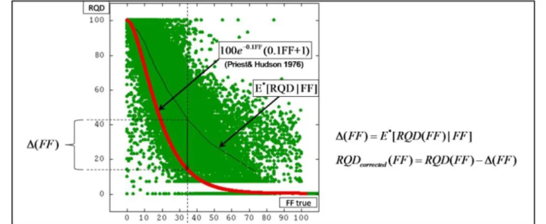
What about RQD compared to FF? Figure 8a shows a scatter diagram between FF (when Terzaghi-corrected) and RQD. The black curve represents the conditional expectation which is, for a given value of FF, the average of the different values of RQD. The behavior predicted by Priest & Hudson’s formula is plotted in red. The least one can say is that this formula does not reflect the experimental average behavior. Does this mean that Priest & Hudson’s hypotheses are not acceptable? Not necessarily because when RQD is compared to FF without the Terzaghi-correction (Figure 8b),
one can see that the formula slightly over-estimates RQD, on average in the range [0, 28], but the differences are not comparable to the previous differences when Terzaghi was applied.
Figure 8. RQD versus FF. Red curve: Priest&Hudson model; black curve: conditional expection of RQD given FF. a) FF is Terzaghi-corrected. b) FF is not Terzaghi-corrected
What happens? Terzaghi correction is necessary to make the discontinuity counting comparable from one direction to another and finally transform the directional number into a counting systematically perpendicular to the fractures. If we do not correct the measurements in this way, we add numbers which are not comparable- the directionality of the measurement makes it non additive when the sampling directions are mixed. For RQD, finally, the problem is the same. The distance between two discontinuities should be corrected according to the angle of the sample with the fractures, so that when we summarize the lengths over 10cm, we summarize quantities that are comparable. This correction was not done and could not be done because the two fractures that delimitate the core length do not necessarily have the same direction; they cannot be classed as the fractures are.
Consequently when we compare an uncorrected RQD with a Terzaghi-corrected FF, we compare two populations that are not comparable because of the correction. When we compare RQD to FF without correction, we compare coherent populations because the bias in the counting is fully compatible with the bias in the associated length and then Priest & Hudson’s formula is verified in an acceptable way.
4.4 Correction trials
From the total amount of data, a sub-set of around 4,500 samples was selected because they have at least 3 fractures with the same direction (or more precisely, belonging to the same angular class). It then becomes possible to correct RQD in the same way as FF, but this time multiplying by the reverse coefficient: 0.26, 0.71 and 0.96 for the classes [0°, 30°], [30°, 60°] and [60°, 90°] respectively. As previously mentioned, and even if we neglect the tolerance linked to the angular class, it is a crude calculation which over-estimates RQD because of the pieces that might become smaller than 10cm when multiplied by the sinus factor. Figures 9 present the results.
Figure 9. RQD versus FF. Red curve: Priest&Hudson model; black curve: conditional expection of RQD given FF. a) FF & RQD are not corrected b) only FF is Terzaghi corrected c) RQD & FF are corrected
We focus on [0, 20] FF interval and Figures 9a and 9b show a zoom of 8b and 8a respectively. When a correction is applied to RQD, it induces so strong a reduction of variability that this time, Priest & Hudson over-estimates RQD given FF when it is Terzaghi-corrected (Figure 9c). So the correction is not efficient, if we refer to Priest & Hudson, and the best solution is certainly not to apply any correction, neither to RQD nor to FF (Figure 9a). It that case, the estimations must be directional as shown previously.
5 Conclusion
The first conclusion is that RQD, as well as FF, are directional measurements that must be estimated after classing the samples according to their directions. Otherwise we mix quantities that are not comparable, producing a not interpretable result. But if we accept this directionality, it means that attributes like RMR become directional too, something which may disturb the practitioner’s habits. If we assume that the directionality of the results is accepted and incorporated in the workflow of dimensioning mining sites, the procedure proposed here, i.e. classing the samples according to their directions is somewhat rudimentary as it proposes estimations only on the sampled directions and no interpolation between these directions. This is a very general problem that occurs when geostatical tools are applied to tensors, and the solution, in the future, is probably to consider the real regionalization space involved by the problem, a 5D space, 3 for the usual coordinates and 2 for the dip crossed by the azimuth, a concept that requires considerable theoretical development because we do not have models for distances crossed by angles.
Now if we want a non directional result, and if we decide to consider Priest & Hudson’s formula as a reference, one possibility is to correct the conditional bias so that Priest & Hudson’s curve and conditional expectation are identical. Consider again the scatter diagram between RQD as it is and Terzaghi-corrected FF.
Figure 10. Proposal for a RQD correction. Red curve: Priest&Hudson model; black curve: conditional expection of RQD given FF. A possible correction is to change RQD so that the
red curve joins the black one. User can choose another model than Prist&Hudson‘s
For each FF, one could remove from RQD the differential between the conditional average and the red curve so that both averages are the same. In other words, the conditional distribution is shifted by a quantity (FF) . This operation requires referring to the Priest & Hudson’s formula but one can choose other references. The idea is to preserve the natural correlation between FF and RQD.
Acknowledgment
The authors would like to acknowledge Codelco, Chile, for their strong support in the implementation of good geostatistical practices along the copper-business value chain, as well as the French governement for supporting half of this work, and anonymous reviewers who greatly contributed to improving the quality of the manuscript. Many thanks to Claudio Rojas and his team of R&T, as well as to the geotechnicians of Chuqui. Without them, nothing would have been possible.
References
Barton N, Lien R, Lunde J (1974) Engineering classification of rock mass for the design of tunnel support. NGI publication 106, Oslo, Rock Mechanics, vol.6 issue 4 pp 189-236
Bear J, Tsang C F, De Marsilly G (1993) Flow and contaminant transport in fractured rock, chapter 4 “Stochastic models of fracture systems and their use in flow and transport modeling“, pp. 169-235, Academic Press, Inc., USA
Bieniawski Z T (1975) The Point Load Test in Geotechnical Practice. Eng. Geol., Sept., pp. 1-11 Deere D U, Hendron A J, Patton JF D, Cording E J (1967) Design of surface and near-surface
construction in rock, Failure and Breakage of Rock, ed. C. Fairhurst, Soc. Of Min. Eng., AIME, N. Y., pp. 237-302.
Goodman R E, Smith H R (1980) RQD and fracture spacing, Journal of the Geotechnical Engineering Diviosn, ASCE 106: 191-193
Jaeger J C, Cook N G W (1969) Fundamentals of Rock Mechanics, Methuen, London. Palmstrom A (1982) T
Priest S D, Hudson J A (1976) Discontinuity Spacings in Rock. J. Rock Mech. Min. Sci. & Geomech, vol. 13, pp. 135-148, Pergamon Press, Great Britain.
Priest S D, Hudson J A (1981)Estimation of Discontinuity Spacing and Trace Length Using Scanline Survey. International Journal of Rock Mechanics and Mining Sciences, vol. 18, pp. 183-197.
Seguret S A, Guajardo C, Freire R (2014) Geostatistical Evaluation of Fracture Frequency and Crushing. In proceedings of Caving 2014, Third International Symposium on Block and Sublevel Caving, Santiago, Chile.
Sen Z, Kazi A (1984) Discontinuity Spacing and RQD Estimates from Finite Length Scanlines, International Journal of Rock Mechanics and Mining Sciences, vol; 21, PP. 203-212.
Stagg K G, Zienkiewicz O C (1968) Rock Mechanics in Engineering Practice, Wiley, N. Y., 442 pp. Terzaghi RD (1965) Sources of error in joint surveys. Geotechnique, vol. 15 issue 3 pp 287-304 Wallis P F, King M S (1980) Discontinuity spacings in a crystalline rock. International Journal of Rock Mechanics and Mining Sciences, vol. 17, pp. 63-66.