Low Delay Transform for High Quality Low Delay Audio Coding

(1)

HAL Id: tel-01205574

https://hal.inria.fr/tel-01205574

Submitted on 25 Sep 2015

HAL is a multi-disciplinary open access archive for the deposit and dissemination of sci-entific research documents, whether they are pub-lished or not. The documents may come from teaching and research institutions in France or abroad, or from public or private research centers.

L’archive ouverte pluridisciplinaire HAL, est destinée au dépôt et à la diffusion de documents scientifiques de niveau recherche, publiés ou non, émanant des établissements d’enseignement et de recherche français ou étrangers, des laboratoires publics ou privés.

Coding

David Virette

To cite this version:

David Virette. Low Delay Transform for High Quality Low Delay Audio Coding. Signal and Image processing. Université de Rennes 1, 2012. English. �tel-01205574�

(2)

N° d’ordre : 2012REN1E014 ANNÉE 2012

THÈSE / UNIVERSITÉ DE RENNES 1

sous le sceau de l’Université Européenne de Bretagne

pour le grade de

DOCTEUR DE L’UNIVERSITÉ DE RENNES 1

Mention : Traitement du signal et télécommunications

Ecole doctorale MATISSE

présentée par

David Virette

préparée à l’unité de recherche (6074 IRISA UMR)

(Institut de Recherche en Informatique et Systèmes Aléatoires)

Étude de

transformées

temps-fréquence pour le

codage audio faible

retard en haute

qualité (Low Delay

Transform for High

Quality Low Delay

Audio Coding)

Thèse soutenue à Rennes le 10 décembre 2012

devant le jury composé de :

Bernd EDLER

Professor Dr.-Ing.

International Audio Laboratories Erlangen / rapporteur

Dominique MASSALOUX

Directrice scientifique adjointe Télécom Bretagne / rapporteur

Sylvain MARCHAND

Professeur des universités

Université Bretagne Occidentale / examinateur

Laurent GIRIN

Professeur des universités Grenoble INP / examinateur

Frédéric BIMBOT

Directeur de Recherche CNRS IRISA / examinateur

Hervé TADDEI

Examinateur OEB / examinateur

Pascal SCALART

Professeur des universités ENSSAT / directeur de thèse

Pierrick PHILIPPE

(3)

(4)

2

Acknowledgments

I would like to express my gratitude to my thesis supervisors Dr. Pierrick Philippe and Prof. Pascal Scalart, for their patience, guidance, enthusiastic encouragement and useful critiques of this research work. I would espe-cially like to thank Pierrick for his unshakeable support and confidence. I have particularly appreciated the long technical and non-technical discus-sions that we had during the course of this research. With him, performing research work can sometimes lead to have the giggles…

Many thanks to Balázs Kövesi, who inspired me part of this work and gave me a different point of view. I would also like to thank Duncan Menzies for his huge help in extensively testing the seamless reconstruction during his M.Eng degree. I am also extremely grateful to Jean-Pierre Petit for encour-aging me to pursue this PhD work.

I would like to thank the reviewers of this thesis, Prof. Bernd Edler and Dr Dominique Massaloux, for their valuable and constructive comments on the manuscript of the thesis. I am also grateful to the members of the Doctorate committee, Prof. Sylvain Marchand, Prof. Laurent Girin, Dr. Frédéric Bim-bot, Dr. Hervé Taddéi, for devoting their time in reading the manuscript and showing interest to this work.

During these years I have had the pleasure to work with great colleagues at France Telecom: Alex, Greg, Rozenn, Jérôme, Marc, Claude, Catherine, Arnault, Martine, Adrien, Ludo, Charles, Florent, Manuel, Alain, Bruno, Stéphane and Stéphane. I have also appreciated the discussions on the “front montant” and “front descendant” of the windows with Hervé and Anisse.

Last but not least, I wish to express my warmest thanks to Katell for en-couraging me and to Elliott, Zélie and Timothé for bringing joy during all these years.

(5)

(6)

4

Abstract

In recent years there has been a phenomenal increase in the number of products and applications which make use of audio coding formats. Among the most successful audio coding schemes, the MPEG-1 Layer III (mp3), the MPEG-2 Advanced Audio Coding (AAC) or its evolution MPEG-4 High Efficiency-Advanced Audio Coding (HE-AAC) can be cited.

More recently, perceptual audio coding has been adapted to achieve coding at low-delay such to become suitable for conversational applications. Tra-ditionally, the use of filter bank such as the Modified Discrete Cosine Transform (MDCT) is a central component of perceptual audio coding and its adaptation to low delay audio coding has become an important research topic. Low delay transforms have been developed in order to retain the per-formance of standard audio coding while reducing dramatically the associ-ated algorithmic delay.

This work presents some elements allowing to better accommodate the de-lay reduction constraint. Among the contributions, a low dede-lay block switching tool which allows the direct transition between long transform and short transform without the insertion of transition window. The same principle has been extended to define new perfect reconstruction conditions for the MDCT with relaxed constraints compared to the original definition. As a consequence, a seamless reconstruction method has been derived to increase the flexibility of transform coding schemes with the possibility to select a transform for a frame independently from its neighbouring frames. Finally, based on this new approach, a new low delay window design pro-cedure has been derived to obtain an analytic definition for a new family of transforms, permitting high quality with a substantial coding delay reduc-tion.

The performance of the proposed transforms has been thoroughly evalu-ated, an evaluation framework involving an objective measurement of the optimal transform sequence is proposed. It confirms the relevance of the proposed transforms used for audio coding. In addition, the new approaches have been successfully applied to the recent standardisation work items, such as the low delay audio coding developed at MPEG (LD-AAC and ELD-AAC) and they have been evaluated with numerous subjective testing, showing a significant improvement of the quality for transient signals. The

(11)

9

new low delay window design has been adopted in G.718, a scalable speech and audio codec standardized in ITU-T and has demonstrated its benefit in terms of delay reduction while maintaining the audio quality of a tradi-tional MDCT.

Keywords: Low delay audio coding – Transform coding – Block switching

(12)

10

List of Figures

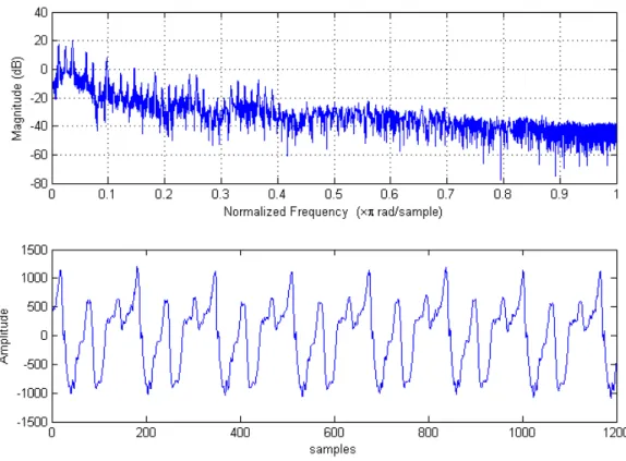
Figure 1 – Frequency and temporal representation of a short segment extracted from

Pitchpipe sequence at 48 kHz sampling rate ... 23

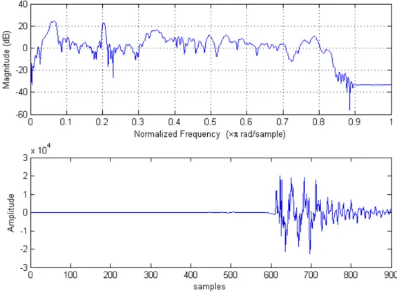
Figure 2 – Short segment extracted from Castanets sequence at 48 kHz sampling rate ... 24

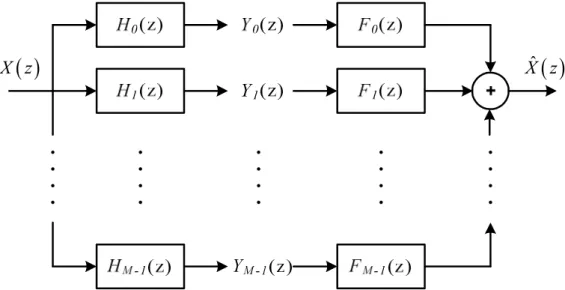
Figure 3 – Structure of filter bank with M sub-bands ... 25

Figure 4 – Maximally decimated uniform filter bank with M sub-bands ... 26

Figure 5 – Polyphase representation of critically sampled analysis and synthesis filter banks ... 30

Figure 6 – General structure of a perceptual audio encoder ... 32

Figure 7 – Frequency masking phenomena ... 37

Figure 8 – Tone masking noise ... 38

Figure 9 – Noise masking tone ... 38

Figure 10 – Temporal masking phenomena... 39

Figure 11 – Uniform scalar quantizer ... 41

Figure 12 – Example of companding function ... 42

Figure 13 – General scheme of predictive scalar quantizer ... 43

Figure 14 – Partitioning based on vector quantization with 24 code vectors (black dots) ... 44

Figure 15 – Arithmetic coding (B-C-B are emitted) ... 46

Figure 16 – Principle of the PAT codec ... 51

Figure 17 – HE-AAC decoder block diagram ... 53

Figure 18 – BCC encoder block diagram ... 54

Figure 19 – Illustration of aliasing terms generated by negative and positive frequency bands in real valued filter bank ... 55

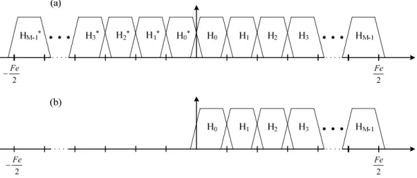
Figure 20 – Illustration of frequency bands in cosine modulated filter bank (a), and complex modulated filter bank (b) ... 56

Figure 21 – Equalization using cosine modulated filter bank... 57

Figure 22 – Equalization using complex-exponential modulated filter bank ... 58

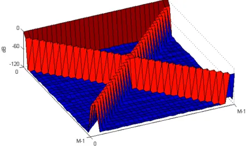
Figure 23 – Magnitude of composite alias component matrix for cosine modulated filter bank ... 58

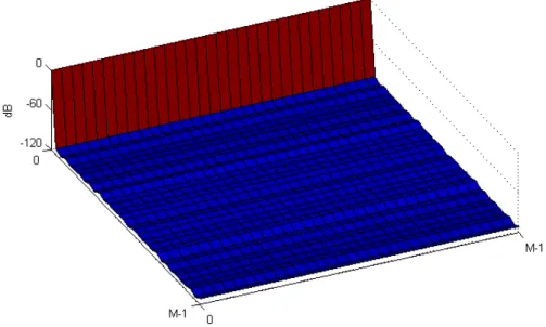
Figure 24 – Magnitude of composite alias component matrix for complex-exponential modulated filter bank ... 59

Figure 25 – Impulse and magnitude response for 1) sine window, 2) Kaiser-Bessel derived window and 3) low overlap window ... 67

Figure 26 – Direct MDCT of multiple consecutive frames of input signal x(n)... 72

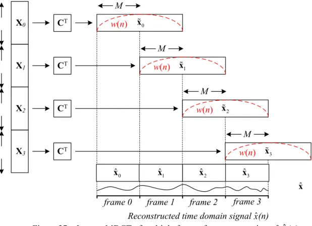
Figure 27 – Inverse MDCT of multiple frames for reconstruction of

ˆx

(n) ... 73

Figure 28 – ELT prototypes for L=KM=2mM with M=32 and m=1, 2, 3, 4 ... 75

(13)

11

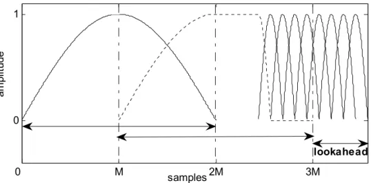
Figure 30 – Comparison of the frequency response of the sine window for the length 2M = 1024 (blue) with the low delay window of length L = 4M = 2048 (red) ... 79 Figure 31 – Combination of windows: long window, transition window (dashed line), and eight short windows ... 81 Figure 32 – Long window (a), Transition windows (b) and (c), and Short window ... 82 Figure 33 – Timing for transition window insertion: the attack arises at the end of the current frame; transition window can be selected when samples 2M to 3M are

processed. ... 84 Figure 34 – Timing for transition window insertion: the attack arises in the next frame; without look-ahead buffer the transition window cannot be anticipated. ... 85 Figure 35 – Eight short windows, each of size 2Ms (dashed line), and the equivalent 2M size window (solid line). ... 91 Figure 36 – Illustration of various window transitions. (a) Traditional window

sequence: long window, long-short transition window (dashed line), eight short windows. (b) Direct transition between long (dashed line) and short (solid line)

windows for the direct transform. (c) Compensation scheme for the inverse transform: in dashed line, the modified part of the long and first short window. ... 94 Figure 37 – Long sine window (a), Transition window (b) and Low delay block switching synthesis window (c) ... 96 Figure 38 – Frequency responses (between the normalized frequencies 0 and 0.1) of transition window (in black) and low delay block switching synthesis window (in red) ... 96 Figure 39 – Frequency responses (between the normalized frequencies 0 and 0.5) of transition window (in black) and low delay block switching synthesis window (in red) ... 97 Figure 40 – Illustration of noise injection in long window for low delay block

switching. ... 98 Figure 41 – Illustration of noise injection in short windows for low delay block switching. ... 99 Figure 42 – LONG_START synthesis window wsynSTART (a), LONG_STOP synthesis window wsynSTOP (b) ... 102 Figure 43 – Long synthesis window in normal operation (blue) and in case of low delay block switching w₁(red). ... 106 Figure 44 – Short synthesis window in normal operation (blue) and in case of low delay block switching w_2s (red). ... 106 Figure 45 – Low delay synthesis window (a), Low delay synthesis window for normal transition between low delay and short sine window (b) and Low delay block

switching synthesis window (c) ... 107 Figure 46 – Frequency responses (between 0 and 0.5) of low delay window (in black) low delay synthesis window for normal transition between low delay and short sine window (in blue) and low delay block switching synthesis window (in red) ... 108 Figure 47 – Symmetric window for direct and inverse MDCT, the sine window (blue) and the Kaiser-Bessel derived (pink) windows are drawn ... 110 Figure 48 – Example of changing window shapes for two consecutive frames ... 112 Figure 49 – Example of changing window shapes for two consecutive frames: (a) analysis windows – (b) synthesis windows ... 114 Figure 50 – Synthesis window initialization (blue) and final synthesis window after correction (pink)... 117 Figure 51 – Low delay analysis (blue) and synthesis (pink) windows ... 117

(14)

12

Figure 52 – Coding gain evolution with the delay reduction in ms (Mz) ... 121

Figure 53 – Attack arising in the first half of the current frame ... 126

Figure 54 – Direct transition between long window and the eight short windows in low delay block switching ... 127

Figure 55 – MUSHRA listening test results for the assessment of LD-AAC with low delay block switching ... 131

Figure 56 – Differential MUSHRA listening test results for the assessment of LD-AAC with low delay block switching ... 133

Figure 57 – First synthesis window sequence for low delay block switching in ELD-AAC ... 134

Figure 58 – Second synthesis window sequence for low delay block switching in ELD-AAC ... 135

Figure 59 – Time alias free zones in low delay block switching reconstruction ... 136

Figure 60 – Time components used for perfect reconstruction in ELD-AAC with low delay block switching ... 137

Figure 61 – Compensation weighting functions w1 and w2 for M = 512 ... 139

Figure 62 – Compensation weighting functions w3 and w4 for M = 512 ... 139

Figure 63 – Results over all items for the ELD-AAC with low delay block switching listening test ... 141

Figure 64 – Results for each of the 7 items with attacks ... 142

Figure 65 – Results for each of the 5 items without attacks ... 142

Figure 66 – CMOS listening test results for the 7 items with block switching ... 143

Figure 67 – CMOS listening test results for the 5 items without block switching .... 143

Figure 68 – CMOS listening test results for the 9 speech items with low delay block switching ... 145

Figure 69 – Low overlap window combinations selected from 5272 set over learning sequence ... 150

Figure 70 – The 12 selected low overlap window combinations ... 151

Figure 71 – Final experimental windows set ... 153

Figure 72 – Windows set used in MPEG 2/4 AAC ... 153

Figure 73 – Representation of non-standard AAC window transitions ... 154

Figure 74 – Block diagram of the G.718 encoder ... 156

Figure 75 – Encoding and decoding timing with ALD window ... 157

Figure 76 – Frequency responses of candidates MDCT windows for G.718 ... 158

Figure 77 – AB listening test results for G.718 with ALD and Sine windows at 16 kbit/s ... 159

Figure 78 – AB listening test results for G.718 with ALD and Sine windows at 32 kbit/s ... 159

Figure 79 – AB listening test results for G.718 with ALD and Sine windows at 16 kbit/s with 8% packet loss... 160

Figure 80 – AB listening test results for G.718 with ALD and Sine windows at 32 kbit/s with 5% packet loss... 161

Figure 81 – ELD-AAC prototype (blue), LONG_START synthesis window (red).. 178

Figure 82 – ELD-AAC prototype (blue), LONG_STOP synthesis window (red) .... 179

Figure 83 – LONG_START sine window (blue), LONG_START ELD-AAC synthesis window (red) ... 179

Figure 84 – First 4 sub-band filters of the analysis ALD transform ... 180

Figure 85 – First 4 sub-band filters of the synthesis ALD transform ... 180

(15)

13

Figure 87 – First band filter for analysis ALD transform (blue), synthesiss ALD

transform (green), MDCT transform with sine window (red) ... 181

Figure 88 – Analysis (blue) and synthesis (pink) ALD transform (band 0) ... 182

(16)

14

List of Tables

Table 1 – Critical bands ... 36 Table 2 – Huffman code example ... 46 Table 3 – Comparison of the performance of the MDCT Sine window, MDCT ALD window, ELT and Low Delay Transform with M=512 ... 119 Table 4 – Comparison of the performance of the MDCT sine window with the maximum theoretical coding gain ... 119 Table 5 – Comparison of the performance of the MDCT ALD window with the maximum theoretical coding gain with Mz = M/4 ... 120 Table 6 – Comparison of the Segmental SNR (dB) performance of the MDCT ALD window with the maximum theoretical coding gain with M=512 and M/4 zeroes ... 120 Table 7 – Supported transition between AAC window sequences ... 129 Table 8 – Test items ... 130 Table 9 – Codecs under test for the LD-AAC with low delay block switching

listening test ... 130 Table 10 – MUSHRA listening test scores for the assessment of LD-AAC with low delay block switching ... 131 Table 11 – Differential MUSHRA listening test scores for the assessment of LD-AAC with low delay block switching ... 132 Table 12 – Codecs under test for the ELD-AAC with low delay block switching listening test ... 140 Table 13 – Mean scores and 95% confidence intervals over all items for the ELD-AAC with low delay block switching listening test... 141 Table 14 – Mean score with 95% confidence interval ... 144 Table 15 – Speech items test set ... 145 Table 16 – CMOS listening test scores for the 9 speech items with low delay block switching ... 146 Table 17 – Segmental SNR (dB) achieved using fixed length sine windows ... 148 Table 18 – Segmental SNR (dB) for adaptive system using 12 combinations of low overlap windows ... 150 Table 19 – Segmental SNR (dB) for final windows set ... 152 Table 20 – Segmental SNR (dB) for final windows set compared to AAC ... 154

(17)

(18)

16

Frequently Used Terms, Abbreviation

and Notations

AAC Advanced Audio Coding

AC Alias Component

BCC Binaural Cue Coding

CELP Code Excited Linear Prediction

CCR Comparison Category Rating

DFT Discrete Fourier Transform

ELD-AAC Enhanced Low Delay - Advanced Audio Coding

ERB Equivalent Rectangular Bandwidth

FFT Fast Fourier Transform

ICC Inter-Channel Coherence

ICLD Inter-Channel Level Difference

ICPD Inter-Channel Phase Difference

ICTD Inter-Channel Time Difference

ITU International Telecommunication Union, –T

(Telecommuni-cation Sector) and –R (Radiocommuni(Telecommuni-cation Sector)

kbit/s Kilo-bit per second

KLT Karhunen-Loève Transform

LD-AAC Low Delay - Advanced Audio Coding

LOT Lapped Orthogonal Transform

LPC Linear Predictive Coding

MDCT Modified Discrete Cosine Transform

MLT Modulated Lapped Transform

MUSHRA MUlti Stimuli with Hidden Reference and Anchors

MPEG Moving Picture Experts Group

NMR Noise to Mask Ratio

PAT Perceptual Audio Transposition

PCA Principal Component Analysis

PQMF Pseudo-Quadrature Mirror Filter

PR Perfect Reconstruction

PS Parametric Stereo

SBR Spectral Band Replication

(19)

17

SNR Signal to Noise Ratio

TDAC Time Domain Aliasing Cancellation

(20)

18

Chapter 1

Introduction

In recent years there has been a phenomenal increase in the number of products and applications making use of audio coding formats. Among the most successful audio coding schemes, MPEG-1 Layer III [ISO 92][Brandenburg 99], the MPEG-2 Advanced Audio Coding (AAC) [ISO 09][Grill 99] or its evolution MPEG-4 High Efficiency-Advanced Audio Coding (HE-AAC and HE-AACv2) [ISO 09][Dietz 02] can be listed. These codecs are based on the perceptual audio coding paradigm. Usually, the perceptual audio codecs find their applications in broadcasting services, streaming or storage. Indeed, historically few delay constraints were im-posed to those audio coding standards and they are consequently not suit-able for conversational applications. As opposed to the broadcast applica-tions, communication services are usually based on speech coding format such as Algebraic Code Excited Linear Prediction (ACELP). The ACELP coding scheme [Schroeder 85] [Adoul 87] is used in the most widely de-ployed communication codecs such as AMR [3GPP 99], 3GPP AMR-WB [3GPP 02] or ITU-T G.729 [ITU-T G.729 96]. This coding algorithm is based on the source-filter model of the speech production and it provides good quality for speech signals with a limited delay which makes it com-patible with conversational applications.

Perceptual audio coding has been adapted to achieve low delay audio cod-ing and to become suitable for conversational applications. The wideband codec ITU-T G.722.1 [ITU-T G.722.1 99] and its superwideband extension ITU-T G.722.1 annex C [ITU-T G.722.1C 05], the MPEG-4 AAC-Low De-lay [Allamanche 99] or the scalable extension of speech codec such as ITU-T G.729.1 [IITU-TU-ITU-T G.729.1 06] [Ragot 07] can be cited. ITU-These communica-tion codecs target not only toll quality for speech signals but also address any audio contents. Consequently the speech production paradigm can not be solely used and transform perceptual coding has been adapted in this application domain.

(21)

19

However, as discussed in this thesis, due to the delay constraint, some of the tools are usually not used in low delay transform codecs leading to quality limitation compared to larger delay perceptual audio codecs. More-over, as most of the delay comes from the transform itself, care must be particularly taken for the window design in order to reduce the algorithmic delay. Some advanced filter bank design has been proposed to reduce the delay associated with the transform [Schuller 00], but they have the draw-back to extend the window or prototype size in order to achieve this delay reduction. A longer prototype leads to a longer temporal noise spreading which increases the risk of perceived noise.

1.1 Thesis motivation

The purpose of this work is to develop coding tools and transform coding schemes that are adapted to low delay audio coding. The quality limitation introduced in perceptual audio coding by the low delay constraint is mainly due to the lack of flexibility in the time-frequency resolution. Indeed, the transform size is fixed with a frame size which is usually between 10 and 20 ms. The overall delay of the transform coding operation lies between 20 and 40 ms. For most of the low bit rate conversational codecs, the 20 ms frame size is used with a reduced sampling frequency (8, 16, 24 or 32 kHz). From this frame size constraint, one can deduce the maximum window size which can be selected. A smaller delay can be obtained, given the trans-form size, for larger sampling rate.

It is known from the successful broadcast perceptual audio codec that the ability to change the time-frequency resolution provides an improved qual-ity for non-stationary sounds and more specifically for transient signals. This thesis presents a time-frequency resolution adaptation scheme, called low delay block switching, which is fully compatible with nowadays trans-form coding and offering this additional transtrans-form flexibility for low delay audio codecs.

A second goal of the thesis was to develop transforms for embed-ded/scalable speech and audio codecs. In this particular context, the core layer is based on ACELP coding with a fixed 20 ms frame size and the transform coding is then used to encode the residual signal. For this spe-cific application, the low delay filter banks introduced in [Schuller 00] are not always efficient as the temporal support is longer than the MDCT and leads to a longer temporal spreading of the quantization noise. Note that the underlying framework is flexible and would allow also shorter temporal support, even if it has not been used in practice. This work presents a low delay window design solution for MDCT. It is based on the relaxation of the perfect reconstruction conditions which have been introduced in [Prin-cen 86]. A general flexible perfect reconstruction system based on the

(22)

20

MDCT is presented and the derivation of new window prototypes is ex-plained.

1.2 Standardization context

This work was closely related to the development of low delay audio cod-ing standards in ISO/MPEG and ITU-T. The technologies which have been proposed during this work have been developed keeping in mind the con-straints which were imposed by the development of MPEG-4 AAC-Enhanced Low Delay (AAC-ELD) and ITU-T Embedded Variable Bit rate (EV-VBR) that led to the G.718 standard and its Superwideband extension G.718 Annex B. The close connection to standardization activity has led to the development of competitive MPEG-4 AAC-LD and AAC-ELD encoder implementations in order to get the possibility to demonstrate the new tools performance and to adapt the encoder accordingly. This development has also required a large amount of work to perform the fine tuning to achieve a state-of-the-art quality which was used to assess the benefit of the pro-posed technologies.

1.3 Contributions and thesis overview

Chapter 2 introduces the basis of perceptual audio coding which is needed to understand the place and role of the coding transform.

Chapter 3 presents a detailed description of the Modified Discrete Cosine Transform (MDCT) which is, by far, the most common transform in per-ceptual audio codecs. It is used as central component for this work. The MDCT and its perfect reconstruction conditions are first defined. Then the associated tools, such as block switching, used for quality improvement with transient signals are presented. It should be noted that most of those tools are exclusively used in broadcast applications in state-of-the-art co-decs due to the additional delay required to ensure a perfect behaviour. The contributions of this work are then presented in Chapter 4. The first tool is the low delay block switching tool for the rapid adaptation of the time-frequency resolution between long transform and short transform without the need of transition windows. This low delay block switching tool has been adapted to the MDCT and low delay filter bank which are used in the low delay MPEG audio codec. The impact of the quantization noise in that context is also discussed.

In section 4.3, the seamless reconstruction method is introduced. This new method allows to develop audio coding schemes without any constraint on window selection and window transition. An audio coding experiment is described to demonstrate the benefit of the method in the context of audio coding with an extended transform windows set. This technique has been adapted to the design of new window prototype for MDCT. In the last part

(23)

21

of the Chapter, a new low delay window design method is introduced. While ensuring the perfect reconstruction, this new window definition pro-vides at the same time a better objective performance compared to tradi-tional low delay window (Low Overlap window) used by MDCT.

Chapter 5 provides the results of the extensive subjective listening assess-ment which were performed in the context of the standardization processes in order to assess the benefit of the proposed method in real world low de-lay audio codecs.

Finally Chapter 6 gives the conclusion with an overview of the thesis document, the contributions of this work and particularly the achievements and the perspective offered by this thesis.

(24)

22

Chapter 2

Filter banks and Transforms in audio

coding

In this chapter, the usage of filter banks and transforms for audio coding is introduced and especially in perceptual audio coding where they are used in many state of the art coding schemes and standards. First, a short introduc-tion of filter banks and transforms is given. Then, an overview of the prin-ciples of perceptual audio coding is presented. As the thesis focuses on conversational applications, care must be taken to obtain good performance for speech content with low delay and low bit rates. Hence, a review of the recently developed parametric tools, which are nowadays widely used in low delay and low bit rate audio coding standards, is provided.

2.1 Filter banks and transforms – an introduction

2.1.1 Characteristics of audio signals

The main characteristic of the audio signal is its wide diversity. All the acoustic signals with a frequency range lying between 20 Hz and 20 kHz can be assimilated to audio signals. However, clear differences between transient and harmonic contents can be perceived. This distinction leads to the definition of two important aspects of audio signals as far as coding is concerned: temporal and frequency aspects.

The main temporal feature of audio signals that has to be taken into ac-count to design a time-frequency transform is its non stationary property. Sounds can be assumed to be pseudo-stationary processes, which means that for short segments (few milliseconds), the short-term stationarity as-sumption can be used. As such the audio signal can be framed into short segments, each processed independently.

(25)

23

An audio signal excerpt extracted from a short segment of Pitchpipe sound is given in Figure 1. It shows the stationarity and periodicity of this highly harmonic signal over a segment of 25 milliseconds (1200 samples at 48 kHz). This gives a perfect example of the stationarity of the sound over short periods. Moreover, this kind of signal has the advantage of being par-ticularly adapted for frequency analysis as the frequency domain signal is mostly represented with a limited number of frequency coefficients. The periodic aspect of this signal facilitates the detection and exploitation of the time redundant components.

Figure 1 – Frequency and temporal representation of a short segment extracted from Pitchpipe sequence at 48 kHz sampling rate

On the contrary, the lack of stationarity in some audio signals is really a problem for the design of a coding scheme, redundancies are inevitably hard to exploit. Indeed, the coding system must be able to adapt automati-cally to quick variations of the signal properties. This second temporal property of audio signals can be defined as potential high dynamic energy variations. In a few milliseconds (ms) time interval, the signal energy may change very quickly. This can be illustrated with a percussive sound that appears just after a period of relative silence. Figure 2 shows a short seg-ment of the castanets audio sequence. As explained in Chapter 3, this kind of audio signal, which is usually referred as transients or attacks, is usually not optimally represented in the frequency domain and special processing must be provided.

(26)

24

Figure 2 – Short segment extracted from Castanets sequence at 48 kHz sam-pling rate

General audio signals can at any time switch between steady states and transition phases. As such the choice of a time-frequency analysis method always involves a fundamental trade-off between time and frequency reso-lution requirements. A filter bank or a transform is used for mapping audio signals from the time domain into the frequency domain. It is often used as a basic component of audio signal processing. In that context, the main fea-ture of a time-frequency transformation is its ability to provide a compact representation of any audio signal by subdividing its content into a compact representation. For this purpose, the time-frequency transformation must maximally reduce the redundancy. However, several aspects of the human audio perception need also to be considered in filter bank audio processing, especially in order to respect both temporal and spectral properties of the audio signal during filter bank processing. Indeed, the perceptual relevance of the time-frequency component of the audio signal and of possible coding artefacts must be considered.

2.1.2 General structure of filter banks

Filter banks and transforms play an important role in audio signal process-ing and perceptual audio codprocess-ing. The input time domain audio signal X(z) is split into several band-limited signals Yk(z) with 0 ≤ k ≤ M – 1 (spectral or sub-band coefficients) obtained through the application of a set of

(27)

analy-25

sis band-pass filters Hk(z). The reconstructed signal X zˆ

( )

is the sum of the recombined sub-band signals filtered via the synthesis filters Fk(z).

Hk(z) and Fk(z) are given by their transfer functions [Bellanger 76]:

( )

( ) ( ) n k k n n k k n H z h n z F z f n z +∞ − =−∞ +∞ − =−∞ = =

∑

(2.1)

Figure 3 illustrates an M sub-bands analysis and synthesis filter bank.

Figure 3 – Structure of filter bank with M sub-bands

A large number of filter banks and transforms can be represented by this basic representation. However, the filter bank displayed on Figure 3 is not suitable for a compact representation of the audio signal: albeit split in relative independent signals, there are more samples in the sub-band do-main than in the full band initial time dodo-main. A decimation operator needs to be introduced to reduce the amount of samples transmitted leading to the introduction of the multi-resolution filter bank theory.

The filter banks which are typically used in audio processing and coding can generally be defined by the maximally decimated filter banks theory in-troduced in [Vaidyanathan 93, Malvar 92b]. Indeed, in that case the number of samples in sub-band domain is equivalent to the number of samples in time domain. For instance, the pseudo-quadrature mirror filter banks (PQMF), the modified discrete cosine transform (MDCT), the modulated lapped transform (MLT) and the lapped orthogonal transforms (LOT) [Bosi 99, Malvar 92b, Shlien 97] can be cited. The MDCT and MLT, which are basically defining the same transform, will be presented in details in Chap-ter 3.

( )

ˆ X z

( )

X z

(28)

26

2.1.3 Maximally decimated filter banks

2.1.3.1 General structure

Following the presentation of the analysis and synthesis filter bank struc-ture, the critically sampled uniform filter banks are introduced now. As every analysis filter output represents only a part of the audio signal width, this signal can be downsampled according to the associated band-width to which it corresponds [Shannon 49]. According to the Nyquist theorem the sampling frequency shall be twice the bandwidth. Figure 4 de-scribes the M sub-bands maximally decimated filter bank processing scheme.

Figure 4 – Maximally decimated uniform filter bank with M sub-bands

The critically sampled uniform filter bank is defined by the set of analysis filters Hk(z) and the associated synthesis filters Fk(z) with 0 ≤ k ≤ M – 1. The output of the k-th analysis filter is obtained by the operation of filter-ing followed by the decimation by a factor of M:

( )

1 1 1 0 1 U H W X W , 0 1 M l l M M k k l z z z k M M − =     = _  _{ } _ ≤ ≤ −    

∑

(2.2)

with W = e j(2π/M). In this equation, only the decimated component given for

l = 0 corresponds to the useful signal, while the other components (l ≠ 0)

represent the frequency shifted version of the input signal spectrum filtered by Hk(z). Those components come from the decimation and are named aliasing components.

Without any processing, the sub-band signal Vk(z) (= Uk(z)) is first interpo-lated and then filtered through the synthesis filters to obtain the sub-band outputs:

( )

1

(

) (

)

( )

0 1 ˆ M M _Wl _Wl _{, 0} ₁ k k k k k l X z V z F z H z X z F z k M M − = = =

∑

≤ ≤ − (2.3) ( ) ˆ X z ( ) X z ( ) 0 ˆ X z ( ) 1 ˆ X z ( ) 1 ˆ M X − z

(29)

27

After summation, the reconstructed signal is given by:

( )

1

( )

1 1

(

)

( )

(

)

0 0 0 1 ˆ M ˆ M M _Wl _Wl k k k k l k X z X z H z F z X z M − − − = = =   = = _ _  

∑

∑ ∑

(2.4)

This can be rewritten as:

( )

1

(

)

1

(

)

( )

1

(

)

( )

0 0 0 1 ˆ M _Wl M _Wl M _Wl k k l l k l X z X z H z F z X z A z M − − − = = =   = _ _=  

∑

(2.5)

where A0(z) is the amplitude distortion affecting the input signal X(z) and

Al(z) for l ≠ 0 are the gains of the lth aliasing terms that are unwanted com-ponents.

The reconstructed spectrum is then a linear combination of the input signal

X(z) and its M – 1 uniformly frequency shifted versions X(zWl). The alias-ing components are then cancelled for 1 ≤ l ≤ M – 1 if:

(

)

( )

1 0 H W F 0 M l k k k z z − = =

∑

(2.6)

The distortion function (amplitude and phase distortion) or transfer func-tion is defined by:

( )

1

( ) ( )

0 0 1 T H F M k k k A z z z z M − = = =

∑

(2.7)

Thus, the filter bank becomes a linear and time invariant system when aliasing is cancelled. The complete system is said to be a Perfect Recon-struction (PR) system if the transfer function corresponds to a pure delay. This condition, which is called paraunitary, is then expressed by:

( )

T z =cz−d. (2.8)

2.1.3.2 Alias component matrix

The aliasing terms can be written as a matrix:

( )

( ) ( )

0 1 1 M A z A z M M z z z A ₋ z      _{ = ⋅} ₌ _⋅         A H f ⋮ (2.9)

(30)

28

where f(z) corresponds to the synthesis filter vector

( )

0 1 1 T M F z F z F − z  

 ⋯  and H(z) is a M × M matrix called the Alias

Component (AC) matrix and is of the form:

( )

(

)

(

)

(

)

(

)

(

)

(

)

0 1 1 0 1 1 1 1 1 0 1 1 M M M M M M H z H z H z H zW H zW H zW z H zW H zW H zW − − − − − −       =         H ⋯ ⋯ ⋮ ⋮ ⋱ ⋮ ⋯ (2.10)

In order to cancel the aliasing terms, Al(z) for 1 ≤ l ≤ M – 1 has to be forced to zero and aliasing cancellation condition can be rewritten as:

( ) ( ) ( )

( )

0 T 0 0 0 0 M A z M z z z z  ⋅   ⋅          ⋅ = = =             H f t ⋮ ⋮ (2.11) with:

( )

( ) ( )

( )

0 1 1 0 0 1 0 1 0 0 0 M 1 F z F z z z z F ₋ z             = =_              f F v ⋯ ⋮ ⋮ ⋱ ⋮ ⋯ (2.12)

The matrix of aliasing gain rewrites as:

( )

z

=

( ) ( ) ( )

z

⋅

z

⋅

z

t

H

F

v

(2.13) And U(z) = H(z).F(z) is defined as the composite alias component matrix:

( )

( ) ( )

( )

( ) (

)

( ) (

)

( )

(

)

( )

(

)

( )

(

)

0 0 1 1 1 1 0 0 1 1 1 1 1 1 1 0 0 1 1 1 1 M M M M M M M M M F z H z F z H z F z H z F z H zW F z H zW F z H zW z F z H zW F z H zW F z H zW − − − − − − − − −       =         U ⋯ ⋯ ⋮ ⋮ ⋱ ⋮ ⋯ (2.14)

As described in equation (2.8), we can go a step further and obtain the per-fect reconstruction by requiring the additional constraint on A0(z) = T(z). The Alias Component matrix notation is useful for the representation of the aliasing terms and is used by some optimization algorithm for filter bank

(31)

29

design when a specific constraint has to be put on the aliasing terms as pre-sented in section 2.3.3.

2.1.3.3 Polyphase representation

Polyphase representations were introduced by Bellanger [Bellanger 76] to facilitate the design of filter banks and their implementations through fast algorithms [Vaidyanathan 93, Malvar 92b]. This theory provides an alter-nate view on the reconstruction process.

The polyphase decomposition of the analysis filter bank, Hk(z), (Type 1 polyphase) and of the synthesis filter bank, Fk(z), (Type 2 polyphase) is used to decompose the analysis and synthesis filters given by their transfer functions, as defined in equation (2.1), into a sum of M terms expressed in the form:

( )

1

( )

0 E M l M k kl l H z z z − − = =

∑

(2.15) and

( )

1 ( 1 )

( )

0 R M M l M k lk l F z z z − − − − = =

∑

(2.16)

Using the matrix notation, the previous equation can be written as:

( )

M

( )

z = z z h E e (2.17)

( )

(M 1)

( )

M z =z− − z z T f eɶ R (2.18) where

( )

z = H0

( )

z H z1

( )

H2

( )

z HM-1

( )

z  T h ⋯ (2.19) and

( )

z = F z0

( )

F z1

( )

F z2

( )

FM-1

( )

z  f ⋯ (2.20) are the analysis and synthesis vectors respectively and the vector e(z) represents the delay chain vector which is expressed in the form:

( )

-1 ( 1)

1 M

z =_ z z− − _

T

e ⋯ (2.21)

The notation eɶ

( )

z , for the matrix e

( )

z , corresponds to eT_*

( )

z−1 where * indi-cates that the components of the matrix are the conjugates.

The matrix E(z) is the M × M polyphase component matrix (also called poly-phase matrix) which is given by:

(32)

30

( )

0,0 0,1 0, -1 1,0 1,1 1, -1 -1,0 -1,1 -1, -1 M M M M M M E z E z E z E z E z E z z E z E z E z       =         T E ⋯ ⋯ ⋮ ⋮ ⋱ ⋮ ⋯ (2.22)

where each row represents one analysis filter. Similarly, the synthesis filter bank can be represented by a polyphase matrix R

( )

z = Rlk

( )

z .

Based on equations (2.17) and (2.18), by migrating the decimation and up-sampling operations before and after the polyphase matrix operations, the polyphase implementation of the analysis and synthesis filter bank can be illustrated by the Figure 5.

Figure 5 – Polyphase representation of critically sampled analysis and synthesis filter banks

In that context of polyphase representation, [Vaidyanathan 93] has shown that the analysis and synthesis filter banks verify the perfect reconstruction condition if and only if the product R(z)E(z) can be written as follows:

( ) ( )

z z cz ₁ z λ − −   = _ _   M-r r 0 I R E I 0 (2.23)

where λ is a positive integer and for some integer r with 0 ≤ r ≤ M – 1. Hence, in order to satisfy the perfect reconstruction constraint, it has been demonstrated by Vaidyanathan that a sufficient condition is r = 0 and the synthesis polyphase matrix has to be the inverse of the analysis polyphase matrix:

( ) ( )

( )

K

( )

z z cz z z z λ − − = = M R E I R Eɶ (2.24) ( ) ˆ X z ( ) X z

(33)

31

K is a positive integer which is selected in order to ensure the causality of

the matrix R(z) and then of the synthesis filter bank. The polyphase repre-sentation is used for some filter banks or transforms definition and proto-type design (as illustrated in paragraph 3.1.3).

2.1.3.4 Cosine modulated filter banks

The cosine modulated filter banks are obtained by the modulation of a low-pass prototype filter h(n) with a cosine function. The main advantage is the possibility to derive low complexity implementations which are based on a simple filtering operation followed by a modulation. The pseudo-QMF (PQMF) filter bank has been introduced by Rothweiler in [Rothweiler 83]. Even if the PQMF does not achieve perfect reconstruction, aliasing compo-nents due to adjacent bands and the phase distortion are cancelled. The per-formance in terms of amplitude distortion depends on the optimization pro-cedure which is used to design the filter bank prototype. Vaidyanathan has proposed several optimization methods to limit the amplitude distortion and shown that using the same definition the perfect reconstruction can be achieved [Vaidyanathan 93].

The impulse responses of the cosine modulated analysis and synthesis filter banks are expressed by:

( )

1

1 cos

,0

1

2

1

1 cos

,0

1

2

k k k k n n n n

L

h

n

k

M

L

f

h

n

k

M

θ θ

π

 _ _ _  +  _ _ _       ₋   _ _ _   

−

=

−

+

≤ ≤

−

=

−

+

≤ ≤

−

(2.25)

where h(n) is the impulse response of the prototype filter of length L,

( )

1 0 1 and 4 k k n L

θ

−

π

≤ ≤ − =

The perfect reconstruction is obtained only if the following conditions are met: 1) L = 2mM, where m is an integer

2) The synthesis filters are given by fk (n) = hk (L – 1 – n) 3) The prototype filter is a linear phase filter h(n) = h(L – 1 – n)

4) The polyphase components of order 2M, noted Gk(z) for 0 ≤ k ≤ 2M – 1, of the prototype filter H(z) must verify the following condition

( ) ( )

( )

constant, 0 1

k k M k M k

Gɶ z G z +Gɶ + z G + z = ≤ ≤k M− (2.26)

Using the order K = 2m – 1 polyphase matrix E(z) of equation (2.23), the condition 4) simply expresses the paraunitary property of this matrix. A co-sine modulated filter bank is then a paraunitary filter bank with the synthe-sis polyphase matrix obtained by:

(34)

32

( )

(2m 1)

( )

z =z− − z

R Eɶ (2.27) Based on this ability to achieve perfect reconstruction, the cosine modu-lated filter banks are widely used in audio signal coding and more specifi-cally for perceptual audio coding.

2.2 Filter banks for perceptual audio coding

The principle of perceptual audio coding consists in reducing the bit rate to represent the audio signal by taking into account the property of the human auditory system. The less relevant components of an audio signal can be quantized with less precision or even completely discarded. Perceptual relevancy is evaluated; this operation relies on the masking phenomena that are described in section 2.2.1. Perceptual audio coding mainly exploits the simultaneous masking which is described in the frequency domain. Hence, these coding schemes are based on filter banks or time-frequency trans-forms leading to a frequency domain representation of the audio signal. This representation holds for both perceptual property interpretation and application of the derived rules. Figure 6 gives a basic block diagram of a perceptual audio coding system.

Figure 6 – General structure of a perceptual audio encoder

The blocks of Figure 6 are described as follows:

Time-frequency analysis: a frequency domain representation requires the

use of a filter bank or a transform to decompose the time domain input au-dio signal into spectral components. This decomposition allows to better isolate the frequency content over each sub-band, this is called energy compaction or energy concentration. Moreover, this time-frequency trans-form decorrelates the sub-band signals and then eliminates some statistical redundancy. The main goal of this filter bank or transform is to divide the signal spectrum into frequency sub-bands or spectral coefficients which can then be conveniently exploited to shape the coding distortion according to

Time-frequency analysis ⋮ Psychoacoustic model Quantization and entropy coding Bitstream 10110111… Audio signal Bit allocation

(35)

33

the auditory model. The main characteristics of a filter bank, which must be carefully evaluated during its design, are listed below:

- Good energy concentration: the basic idea in a data reduction scheme is to filter the signal into various sub-band signals. Instead of quantizing the samples of the signal with desired number of bits per sample, the quantiza-tion can be performed on the transform coefficients with a different number of bits for each. The total number of bits should be the same, but the mean square error is lower in the transform coding case compared to quantizing the samples in the time domain as the system can allocate the bits accord-ing to the spectrum characteristics.

- Signal adaptive time-frequency tiling: the audio signal is composed of stationary and transient parts. An audio coding scheme must adapt to the time- frequency content of the signal.

- Perfect or near-perfect reconstruction: this characteristic is important in order to recover the original audio signal at the decoding stage, or at least to approach its reconstruction, this is important, especially for higher rates (any reconstruction quality can be achieved, and transparent coding quality obtained).

- Critically sampled: each band-pass filter is sub-sampled by a factor corre-sponding to the number of sub-bands. No increase in terms of components to be encoded is required for efficient compression applications. In these systems, the overall rate at the output of the analysis stage equals the over-all rate at the input of the analysis stage.

- Limited blocking artefacts: the audio signal is processed by blocks or frames. The reconstruction must ensure a smoothed transition from one block to the other.

- Good sub-band separation and stop-band attenuation: This characteristic corresponds to the minimum attenuation which can be obtained with a fil-ter. It ensures a good separation between the sub-band to reduce the redun-dancy.

Psychoacoustic model: it aims at representing the behaviour of the human

auditory system. Based on the input signal, a perceptual model, also known as psychoacoustic model, is used to estimate the perceptual masking threshold based on the simultaneous masking and in quiet masking phe-nomena [Zwicker 07]. Two slightly different effects are usually considered depending on the tonality characteristic of the masker. This model provides the necessary indication on how to inject quantization noise during the cod-ing stage. This perceptual model relies on the time-frequency analysis of the audio signal if the frequency resolution is sufficient. Otherwise, a dedi-cated Discrete Fourier Transform (DFT) is directly applied to the time do-main input signal in order to obtain an adequate frequency representation.

(36)

34

Quantization and entropy coding: the quantization stage associated with

an efficient coding scheme aims at reducing the bit rate required to repre-sent the audio signal. The sub-band signal is approximated on a reduced number of levels (quantization levels) and an indication of the selected level is further compacted using an entropy-coding scheme. This quantiza-tion step is applied in accordance with bit allocaquantiza-tion based on the psycho-acoustic masking properties. The spectral coefficients are then quantized with the objective of hiding the quantization noise just below the masking threshold, according to the decision performed during bit allocation.

Bit allocation: this procedure distributes the available bit budget, driven by

the coding bit rate, in all the frequency sub-bands. It determines the amount of bits that each sub-band must receive in order to shape the quantization noise according to the perceptual model. The bit allocation is carried out based on the masking curve obtained from the perceptual model.

The basic components of an audio coding scheme are further described hereunder.

2.2.1 Perceptual model

In order to have a bit rate reduction guided by perception, transform coding is based on a perceptual model indicating how the spectrum of the quanti-zation noise can be shaped. The main goal of the perceptual model is to de-scribe as precisely as possible how the sound and the quantization noise might be perceived by the human auditory system.

2.2.1.1 Absolute threshold of hearing

Based on listening tests and experiments [Zwicker 07], it is considered that the human auditory system is able to perceive sound in the frequency range of 20 Hz – 20 kHz. However, the ear is not equally sensitive at all the fre-quencies. The hearing area is the region in the Sound Pressure Level (SPL)/frequency plane in which the sound is audible. It is defined as the region in which listeners can perceive a stimulus made of a pure tone or a narrow band noise in a noiseless environment, and the lower energy level for which this stimulus can be heard defines the absolute threshold of hear-ing. The threshold of hearing, also called the threshold in quiet, can be ap-proximated by:

( )

(

)

_0.8 ( )2

₍

₎

₄ 0.6 /1000 3.3 3 3.64 / 1000 6.5 f 10 / 1000 (dB ) q T f = f − − e− − + − f SPL (2.28)

where f is the frequency in Hz and the absolute threshold of hearing in dB

SPL. It is represented on Figure 8. It can be seen that the human auditory

(37)

35

higher frequencies the curve increases exponentially and only a sound with a significant level of energy can be perceived. It is particularly difficult to hear sounds above 16 kHz where only sounds with energy levels higher than 60 dB SPL are perceived.

2.2.1.2 Critical bands

The concept of critical bands, introduced by Fletcher [Fletcher 40], is par-ticularly important in psychoacoustic. The loudness perceived in a critical band corresponds to the integration of the loudness for all the frequency components of that band. When measuring the hearing threshold of a nar-row band noise as a function of its bandwidth while keeping its overall pressure level constant, this threshold remains constant as long as the bandwidth does not exceed the critical bandwidth. When exceeding the critical bandwidth, the hearing threshold of the noise increases.

Critical bands play a role in sound intensity perception and are also related to masking phenomena. If a sound is presented simultaneously with mask-ers, the maximum masking contribution is obtained only when the masking components fall within the same critical band. The masking property is then constant over critical bandwidths and drop rapidly outside this band. Moreover, the perceived loudness of a sound is independent of its band-width as long as it is smaller than the corresponding critical bandband-width. Zwicker and Fastl [Zwicker 07] have proposed an analytic expression of critical bandwidths as a function of their centre frequencies:

(

)

2 0.69

25 75 1 1.4 0.001 _c

f  f 

∆ = + _ + _ (2.29)

Table 1 lists the bands used to model the human ear in the form of a filter bank with 24 abutting critical bands. It is typically used for audio coding applications. A new frequency scale has been introduced, the Bark scale, which follows the critical band rate and has a unit “Bark”. According to this scale, 1 Bark defines the lower and upper limits of each critical band. The Bark scale is then a mapping of frequencies onto a relation Herz/Bark. This relation is almost linear up to 500 Hz and then becomes quasi loga-rithmic. The critical band rate z(f) (expressed in Bark) can be approximated using the following expression from [Zwicker 07]:

( )

13arctan 0.00076

(

)

3.5 arctan 2 7500 f z f = f +          (2.30)

Several alternative methods have been used to simulate the hearing fre-quency scale leading to alternative definitions. Moore and Glasberg [Moore 03] have proposed to replace the Bark scale by what they call the

(38)

Equiva-36

lent Rectangular Bandwidth (ERB) scale. The ERB scale is defined as the

number of ERBs below each frequency:

( )

21.4 4.37 1 1000 f ERBS f = _ _ _+ _     (2.31)

f is expressed in Hertz. And the critical bandwidth/ERB is given by:

( )

0.108 24.7

ERB f = f + (2.32)

Table 1 – Critical bands

2.2.1.3 Temporal and frequency masking

Several perception criteria are used to reduce the quantity of data to be stored or transmitted without any degradation of the subjective audio qual-ity. Two kinds of masking phenomena can be experienced and are pre-sented in this section: frequency masking (also known as simultaneous masking) and temporal masking.

Frequency masking is commonly used in audio coding schemes. The mask-ing curves are used to distribute the quantization noise below the percep-tual masking threshold. Temporal masking offers a more limited interest for the perceptual audio coding as it is more difficult to exploit. Masking models are usually not exploiting the temporal masking. However, the per-ceptual audio coding models must ensure a sufficient temporal

concentra-Critical band index Centred frequency (Hz) Critical bandwidths (Hz) Lower frequency limit (Hz) Upper frequency limit (Hz) 1 2 3 4 5 6 7 8 9 10 11 12 13 14 15 16 17 18 19 20 21 22 23 24 50 150 250 350 450 570 700 840 1000 1170 1370 1600 1850 2150 2500 2900 3400 4000 4800 5800 7000 8500 10500 13500 100 100 100 100 110 120 140 150 160 190 210 240 280 320 380 450 550 700 900 1100 1300 1800 2500 3500 0 100 200 300 400 510 630 770 920 1080 1270 1480 1720 2000 2320 2700 3150 3700 4400 5300 6400 7700 9500 12000 100 200 300 400 510 630 770 920 1080 1270 1480 1720 2000 2320 2700 3150 3700 4400 5300 6400 7700 9500 12000 15500

(39)

37

tion of the quantization noise and the filter banks are usually designed to provide this time-frequency resolution trade-off as it will be explained in section 3.2.

Frequency masking

The first phenomenon is defined as frequency masking or simultaneous masking. It occurs when a so-called masker masks simultaneous signals presented at the auditory system and more specifically when stimuli are present at nearby frequencies. The curve, represented in Figure 7 as mask-ing threshold, describes the modified audibility threshold in presence of some masking signal. This curve is based on the absolute threshold of hear-ing, on top of which, with the additional presence of the masker, the mask-ing threshold is modified. Two kinds of maskers are commonly used to de-rive the masking curve: maskers made of pure tones and of band limited noise. Both are studied to measure their capability at masking (quantiza-tion) noise.

Figure 7 – Frequency masking phenomena

The first simultaneous masking phenomenon is defined as tone-masking-noise. In this first category of frequency masking, a pure tone in a critical band masks a band limited noise as long as this noise belongs to the same critical band. The minimum signal-to-mask ratio (SMR), which represents the smallest difference between the intensity of the masking signal and the intensity of the masked signal, tends to lie between 21 and 28 dB. In the example provided in Figure 8, a noise of one Bark bandwidth centred on the central frequency of the critical band is masked by a pure tone of 80 dB at the same central frequency.

101 102 103 104 105 −20 0 20 40 60 80 100 120 140 160 180 Fréquences (Hz) Niveau (dB SPL) Absolute Threshold of Hearing Masker Masking Threshold Masked sound Frequency (Hz) S o u n d P re s s u re L e v e l ( d B )

Low Delay Transform for High Quality Low Delay Audio Coding

HAL Id: tel-01205574

https://hal.inria.fr/tel-01205574

Coding

David Virette

To cite this version:

THÈSE / UNIVERSITÉ DE RENNES 1

DOCTEUR DE L’UNIVERSITÉ DE RENNES 1

Ecole doctorale MATISSE

David Virette

préparée à l’unité de recherche (6074 IRISA UMR)

(Institut de Recherche en Informatique et Systèmes Aléatoires)

Étude de

transformées

temps-fréquence pour le

codage audio faible

retard en haute

qualité (Low Delay

Transform for High

Quality Low Delay

Audio Coding)

Acknowledgments

Contents

Abstract

List of Figures

ˆx

List of Tables

Frequently Used Terms, Abbreviation

and Notations

Chapter 1

Introduction

1.1

Thesis motivation

1.2

Standardization context

1.3

Contributions and thesis overview

Chapter 2

Filter banks and Transforms in audio

coding

2.1

Filter banks and transforms – an introduction

2.1.1 Characteristics of audio signals

2.1.2 General structure of filter banks

( )

( )

( )

∑

∑

( )

( )

2.1.3 Maximally decimated filter banks

2.1.3.1 General structure

( )

∑

( )

( )

( )

(

) (

)

( )

∑

( )

( )

(

)

( )

(

)

∑

∑ ∑

( )

(

)

(

)

( )

(

)