GDP ESTIMATES FOR REGIONS WITHIN THE PROVINCE OF
QUEBEC: THE CHANGING GEOGRAPHY OF ECONOMIC ACTIVITY
André Lemelin, Pierre Mainguy, Danielle Bilodeau and Réjean Aubé
Inédit / Working paper, no 2011-08
GDP ESTIMATES FOR REGIONS WITHIN THE PROVINCE OF QUEBEC: THE CHANGING GEOGRAPHY OF ECONOMIC ACTIVITY*
André Lemelin, Pierre Mainguy, Danielle Bilodeau and Réjean Aubé
This paper is a preliminary version of a chapter in the following book: Esteban Fernández-Vasquez and Fernando Rubiera -Morollón (eds.)
«Rethinking the economic region. New possibilities of regional anal ysis from data at small scale»
Advances in Spatial Economics, Springer (forthcoming)
The views and opinions expressed herein are those of the authors and do not necessarily reflect
the views of the Institut de la statistique du Québ ec
Institut national de la recherche scientifique Centre - Urbanisation Culture Société
Montreal
André Lemelin
Professor-Researcher, Université du Québec, INRS-UCS
Pierre Mainguy
Consultant
Danielle Bilodeau
Institut de la statistique du Québec, Direction des statistiques économiques et du développement durable
Réjean Aubé
Institut de la statistique du Québec, Direction des statistiques économiques et du développement durable
Centre - Urbanisation Culture Société Institut national de la recherche scientifique 385, Sherbrooke Street East
Montreal (Quebec) H2X 1E3 Phone: (514) 499-4000 Fax: (514) 499-4065
www.ucs.inrs.ca
This document can be downloaded without cost at:
www.ucs.inrs.ca/sites/default/files/centre_ucs/pdf/Inedit08 -11.pdf
Abstract
The purpose of this paper is twofold: report on the method developed at the Institut de la statistique du Québec (ISQ) to estimate regional GDP; analyse the data to examine recent changes in the geographical distribution of economic activity in Quebec.
The ISQ method for estimating regional GDP is a top-down one, allocating three components of value added by industry (GDP) among regions, using allocators constructed from fiscal data of the Quebec ministry of revenue. The method is applied to the 17 administrative regions and 6 metropolitan areas in Quebec, from 1997 onwards.
The evolution of regional shares of population, GDP and personal income is examined from the core-periphery perspective, reorganizing the data to create analytical regions adequate for that purpose. For all three dimensions, the shares of regions traditionally considered as peripheral are falling. There is also a redistribution from non-metropolitan to metropolitan areas. Finally, there is movement out of Île de Montréal towards the rest of the metropolitan area and its outer ring. The analysis is extended to a shift-share decomposition of GDP growth, but the residual component of differential growth overweighs the structural component in most cases.
Key Words:
Regional economic activity; Regional GDP estimation; National accounting for regions JEL classification: R12; C82; E01
Résumé
L’objectif de cet article est double: présenter la méthode de l’Institut de la statistique du Québec pour estimer le PIB régional; examiner l’évolution récente de la distribution géographique de l’activité économique au Québec.
La méthode d’estimation du PIB régional de l’ISQ est une une méthode descendante: trois composantes de la valeur ajoutée par industrie (PIB) sont réparties entre les régions au moyen d’allocateurs construits à partir de données fiscales de Revenu Québec. La méthode est appliquée aux 17 régions administratives et aux 6 régions métropolitaines du Québec, à partir de 1997. L’évolution des parts régionales de la population, du PIB et du revenu personnel est examiné selon la logique centre-périphérie, après que les données aient été réorganisées pour créer des régions analytiques pertinentes à cette fin. À tous égards, les parts des régions traditionnellement considérées comme périphériques diminuent. Il y a aussi une redistribution des régions non métropolitaines vers les régions métropolitaines. Enfin, il y a un déplacement à partir de l’Île de
Montréal vers le reste de la région métropolitaine et sa couronne externe. L’analyse est prolongée par une décomposition structurelle-résiduelle de la croissance du PIB, mais la composante résiduelle domine la composante structurelle dans la plupart des cas.
Mots clés :
INTRODUCTION
The purpose of this paper is twofold. First, we report on a method developed at the Institut de la Statistique du Québec (ISQ) to estimate the GDP of regions within the Province of Quebec. And, second, we analyse the estimates to examine the recent evolution of the geographical pattern of economic activity in Quebec.
There are two families of methods for calculating regional GDP. So-called “bottom-up” methods consist in collecting economic data at the individual production-unit level (establishment), and then adding them up to obtain the corresponding regional data. Various adjustments are then performed in order to make the regional data consistent with national data, so that the sum of regional products is equal to total production over the national territory. So-called “top-down” methods consist in allocating an overall national figure across regions. They do not require knowledge of local establishment data. The national figure is distributed using an indicator which is as close as possible to the variable to be estimated. Practically speaking, most methods are mixed. For, on the one hand, the kind of data required for bottom-up estimation almost always has gaps that must be filled using a top-down method. And, on the other hand, top-down methods also make use of exhaustive data sources similar to those required by bottom-up methods.
A BRIEF SURVEY OF M ETHODS1
There are few examples of regional GDP computed for entities smaller than States or provinces, except in the European Union (see below). In Canada, the Conference Board produces annual estimates of the GDP of metropolitan areas (MAs)2,3. The Conference Board first estimates gross value added at basic prices in real terms (at constant prices) for some sixty industries (depending on the information available for each MA), using monthly employment data from Statistics Canada’s Labour Force Survey (LFS). Metropolitan GDP is then obtained as the sum of gross value added over industries. But the LFS generates data on a place-of-residence basis, rather than on a place-of-work basis, whereas GDP is defined, according to national accounting principles, in terms of where production takes place. So the Conference Board method adjusts its employment figures to take commuting into account, using population census data: employment in a MA is obtained by multiplying the LFS figure by the ratio of the number of workers whose place of employment is in the MA, over the number of workers whose residence is in the MA. Industry gross value added is obtained by multiplying estimated employment in each MA by labour
1
For a more detailed survey, see Lemelin and Mainguy (2009b).
2
Technically, Census Metropolitan Areas (CMAs), follow ing the statistical system in Canada. It is understood that, throughout this text, metropolitan areas are Census Metropolitan Areas. We shall use the full expression « Census Metropolitan Areas » w hen discussing the definition of MA boundaries by Statistics Canada.
3
Those estimates are published in the spring issue of the Conference Board’s quarterly Metropolitan Outlook/Note de conjoncture métropolitaine.
productivity at the Provincial level. So the underlying hypothesis is that labour productivity is the same within any industry everywhere in a given Province. This may constitute a weakness in the case of industries encompassing a wide range of activities when the mix of activities varies from one region to another. Finally, the Conference Board method could hardly be applied to all regions, given that LFS data are unreliable for small regions (or, for that matter, for small industries), because of high error margins in small sub-populations, not to mention Statistic Canada’s confidentiality rules, which can result in masked data4
.
In the United-States, until recently, the Bureau of Economic Analysis (BEA) did not estimate GDP at a lesser scale than the State level5. However, since September 2007, the BEA publishes GDP estimates for metropolitan areas6. The BEA methodology (Panek et al., 2007) uses a top-down approach, distributing state-level output by industry to metropolitan areas according to earnings (reported by place of work). Earnings – which consists of wage and salary disbursements, supplements to wages and salaries, and proprietors’ income – are estimated on the basis of data from the Quarterly Census of Employment and Wages of the Bureau of Labor Statistics (BLS). The BEA also produces statistics on personal income for counties. Now, personal income is the sum of incomes of persons who live in a given area. Since county personal income is computed mostly from data collected on a place-of-work basis, the BEA applies a correction using decennial census data on home-to-work commuting. The adjustment is interpolated or extrapolated to non-census years, following a method described in BEA (2008). Within the European Union, the rules for distributing so-called “structural” funds (in support of poorer regions) requires knowing regional GDP. Calculations follow common principles laid down by Eurostat, the EU statistical agency. But it must be kept in mind that the regions of Europe are of a much greater demographic and economic weight than most of Quebec’s 17 administrative regions. Particular attention was paid to the techniques of the French Institut
National de la Statistique et des Études Économiques (INSEE), and of the UK Office for
National Statistics (ONS).
In France, INSEE applies a method which rests on a complex system of enterprise data, and calls upon the expertise of “regional accountants”, whose local presence and knowledge of the
environment make it possible to better validate the information (Delisle, 2000)7. The INSEE
4
Statistics Canada defines a minimum threshold below w hich no information may be disseminated (Statistics Canada, 2011, 71-543-G, p. 31, “Release criteria”). For Quebec, that threshold is 1500. It follow s that for small CMAs, some industries “disappear” at times, only to reappear later on, just because the number of employees has temporarily fallen below the confidentiality threshold. This limits the level of detail at w hich the method is applicable and occasionally forces to make adjustments.
5 The BEA method for computing Gross State Products (GSP), like Statistics Canada’s method for provincial GDP, is a mixed,
bottom-up/top-dow n method w hich makes use of fiscal and administrative data.
6
Panek et al., 2007. The 2001-2009 estimates of GDP by metropolitan area in current and real (chained) dollars are available from the Regional Economic Accounts page of the BEA Web site at w w w .bea.gov/regional/index.htm.
method is mixed, but predominantly bottom-up. It would seem to be more accurate than the ONS’s (described below), but also more demanding. That is probably why it is fully applied only for certain benchmark years, on the basis of which other years are estimated by inter- or extrapolation.
In the United Kingdom, the ONS applies a method which is quite similar to that of the US BEA for estimating GSP, and to that of Statistics Canada for provincial GDP. It appears however that the top-down side is more important in the ONS method (Lacey, 2000). The main shortcoming of that method is that wages and salaries are allocated on a place-of-residence basis, rather than on a place-of-work basis, as the concept of gross domestic product implies. On the other hand, the data requirements of the ONS method are moderate, especially when compared to INSEE’s. The method developed for estimating the GDP of Quebec’s 17 administrative regions and 6 metropolitan areas is described in greater detail in the next section. It is a mixed method, closely akin to that of the ONS in the UK. Regional GDP at basic prices is computed by industry or group of industries, following the income-based approach, defined in the OECD System of National Accounts as the sum of components of value added (OECD, 2001). Roughly speaking, it consists in allocating total labour income and net income of unincorporated business (NIUB – also called “mixed income”) by industry among regions using allocators8
constructed from fiscal data on wages and salaries and NIUB compiled by Revenu Québec (the Quebec ministry of revenue, responsible for tax collection). For each industry, other components of value added (corporation profits, interest, capital consumption allowances, inventory valuation adjustment, and net indirect taxes on production) are then distributed in proportion to the sum of total labour income and NIUB.
The key ingredients in the method are a compilation of fiscal data on incomes, and reliable home-to-work commuting tables by industry. We believe a similar approach could be used to estimate regional GDP anywhere these are available. Our method has the advantage of being less limited than the Conference Board method by small-region or small-industry sampling errors in labour survey data, and it implicitely takes into account inter-regional productivity differences within industries, since it relies on income, rather than employment data. Compared to the French INSEE method, ours is certainly less demanding. And compared to the British ONS method, it is consistent with the GDP place-of-production definition, and it has the advantage of using all of the detailed fiscal data, rather than the 1% sample of tax records, compiled by Inland Revenue. We now proceed to give a more complete account of the method. In section 2, we will examine the evolution of regional GDP from the core-periphery perspective.
ISQ REGIONAL GDP ESTIMATION METHOD
BROAD OUTLINE
The process of applying the method can be summarized as follows:
1. The starting point is the Quebec total, to be allocated between the regions: value added (VA) at basic prices, by industry and by component, in current dollars, according to Quebec Economic Accounts. They are the “target data”.
2. Data on regional distribution are obtained from Revenu Québec, which extracts them from individual income tax returns:
Wages and salaries, by administrative region of residence and by Standard
Industrial Classification (SIC) industry;
NIUB, by administrative region of residence and by SIC industry until 2000, and by North-American Industry Classification System (NAICS) industry afterwards. 3. Revenu Québec data undergoes two conversions before being used to form allocators:
Data by SIC industry are converted to the NAICS.
Place-of-residence fiscal data are converted to place-of-work data using
home-to-work commuting patterns by industry (special tabulation by Statistics Canada, based on population census data).
4. The table of NIUB by NAICS industry and by region is adjusted, applying the minimum-information-gain method (also known as minimum cross-entropy), so as to exploit all of the information in Revenu Québec’s fiscal data, accommodating for the relatively high rate of missing information relating to industry of origin. That procedure makes it possible to use NIUB data for which the region of residence is known, but not the industry.
5. Wages and salaries and adjusted NIUB, by industry and by region, are used as allocators for the other components of VA:
supplementary labour income is distributed in proportion to salaries;
other components are distributed in proportion to the total of salaries,
supplementary labour income, and NIUB.
6. VA by administrative region (that is, regional GDP) is obtained by first summing the components within each industry, and then summing the VA of industries.
In addition, eight industries are treated in a special way: Fishing, hunting and trapping; Metal ore mining; Non-metallic mineral mining and quarrying; Construction; Petroleum and coal products manufacturing; Primary metal manufacturing; Lessors of real estate property; Owner-occupied dwellings. We shall come back to those later. Finally, the top-down approach of the method ensures that estimated regional GDP is consistent with provincial economic accounts.
GEOGRAPHICAL DIVISIONS IN THE ESTIM ATION PROCESS
The Province of Quebec is divided into 17 administrative regions (AR). There are also 21 regional conferences of elected officials (Conférences Régionales des Élus – CRÉ), where the mayors and prefects of the region meet (since it is an institution unique to Quebec, we shall not attempt a translation, and will henceforth use the acronym CRÉ). Fifteen of the 17 administrative regions coincide with the territory of a single CRÉ, but two of them have three each. Besides the administrative regions, there are six metropolitan areas (MA) in Quebec. Two of the administrative regions are entirely included within the Montreal metropolitan area, while seven others are partly inside, partly outside a metropolitan area. Finally, one metropolitan area, Gatineau, is part of the larger Ottawa-Gatineau metropolitan area which extends into the neighboring Province of Ontario.
The objective in producing regional data was to provide local authorities with information on which to base their development strategies. So it was desirable to estimate GDP for all of the territorial divisions described above. To make that possible, the Quebec territory was subdivided
into 30 areas which can be aggregated into administrative regions, CRÉ territories9, or
metropolitan areas. The map in Figure 1 displays the geographical divisions. It was possible to obtain the target data and the Revenu Québec fiscal data for each of the 30 territories. So the GDP estimates are perfectly consistent for any aggregation of the 30 territorial subdivisions. However, for the eight special industries mentioned above, two separate calculations must be made, one for the 17 administrative regions, with one of them divided into three regional conferences, and another for the 6 metropolitan areas and the non-metropolitan territories.
STEPS IN THE ESTIM ATION PROCESS
This section examines the estimation process in greater detail10. In what follows, we consider successively: source data used (target data on GDP by industry, and Revenu Québec fiscal data); prior processing applied to Revenu Québec data to construct the allocators; and application of the allocators to the target data.
9
Except for the three regional conferences of the Nord-du-Québec administrative region, w hose economic and demographic w eight is too small to subdivide the region.
Target data on GDP by industry
Data on GDP by industry and by component for Quebec as a whole are the “target data”, which are to be distributed among regions by the estimation process. Indeed, the estimation results must be consistent with other official data. Such consistency is ensured because the totals distributed among regions with allocators correspond to the official figures. However, these target data are not drawn as such from a single source; rather, they are constructed from three main sources:
GDP at basic prices, in current dollars, by industry and by province, in current dollars (Statistics Canada, Provincial Gross Domestic Product by Industry, 15-203-XIE);
Statistics Canada’s Provincial Input-Output tables (IO) for Quebec;
GDP at basic prices, by component, for 18 industry groups, in current dollars, estimated by the Institut de la statistique du Québec (Comptes économiques des revenus et dépenses
du Québec).
Industry GDP at basic prices in current dollars is consistent with Economic Accounts. So it is a good starting point for estimating regional GDP by a top-down method. Indeed, the choice of estimating regional GDP in current, rather than constant, dollars was made with the purpose of obtaining a regional GDP which is consistent with Economic Accounts. Moreover, the regional GDP estimation method uses allocators based on Revenu Québec fiscal statistics, which are, obviously, in current dollars.
The level of aggregation chosen for the estimation of regional GDP is 63 NAICS industries. At that level of detail, however, the first source does not disaggregate industry GDP into its components. So if one were to rely on that single source, one would be forced to apply the same regional allocator to all of each industry’s value added. For that reason, industry GDP data are used jointly with data from other sources.
In Comptes économiques des revenus et dépenses du Québec, the Institut de la statistique du Québec publishes the value of GDP at basic prices for 18 industry groups, with three components: total labour income (wages and salaries, plus supplementary labour income); gross operating surplus and miscellaneous adjustments; and the total of accrued net income of farm operators from farm production and net income of non-farm unincorporated business, including rent (mixed income).
These data are utilized jointly with the input-output tables, to overcome certain classification and Economic Account benchmarking problems, and to obtain the necessary information to distribute the GDP of the 63 industries between the three value added components mentioned earlier. The result of those adjustments constitutes what we call the “Economic Accounts target data”.
Target data for recent years
The source data on GDP by industry is published with a certain time-lag, and in several stages: preliminary estimates, revised estimates, etc. The definitive figures are often published only after several years. Consequently, the target data for the estimation of regional GDP in recent years must be projected on the basis of available source data, and the GDP estimates are revised as better and more complete data become available. For example, in May 2011, regional GDP figures on the Institut de la statistique du Québec Web site are those published in late 2010, and it is specified that11:
2009 (year t–1 relative to 2010) values are preliminary estimates;
2008 (year t–2) values are estimates;
2007 (year t–3) values are revised estimates;
2006 (year t–4) values are provisional figures;
2005 (year t–5) values are revised figures;
2004 (year t–6) values are definitive figures.
Practically speaking, target data for year t–5 (2005), published in late 2010, have been revised since the 2009 release, but they are expected to be definitive; and target data for year t–4 (2006) are subject to revisions that are expected to be minor. Therefore, these target data are considered to be quite reliable. To establish the target data for years t–3 and t–2 (2007 and 2008), neither Statistics Canada’s Provincial Input-Output tables, nor its GDP at basic prices, by industry and by province, are available. So the target data are constructed from the ISQ estimates of GDP at basic prices, by component, for 18 industry groups (in Comptes économiques des revenus et dépenses
du Québec), using a combination of disaggregation and projections based on the evolution of real
GDP. These estimates are considered to be reasonably reliable, but somewhat less so than those of years t–4. Finally, for year t–1, even the 18-industry group GDP estimates are not yet available, and the target data are established by projecting t-2 estimates according to the evolution of real GDP. These are indeed preliminary estimates.
11
Statistics Canada and ISQ are in the process of review ing their revision policies, so the sequence presented here is subject to change.
Revenu Québec fiscal data
Revenu Québec fiscal data on salaries and individual business income are used to construct the allocators according to which the target values are distributed between regions. So they are the two main allocators utilized. Other allocators are used for special industries.
Salaries
Fiscal data on salaries are compiled by Revenu Québec, and passed on to the Institut de la Statistique du Québec in an aggregated form that complies with the confidentiality rules which protect personal information. The data are extracted from R1 slips12 (equivalent to Canadian federal T4 slips). By combining the amounts of worker incomes according to the R1 slips, employer economic activity codes, and employees’ postal codes, Revenu Québec produces an estimate of the amount of salaries by activity and by territory of employee residence.
Those data are quite complete. For instance, in 1997, Revenu Québec was able to determine taxpayer territory of residence and employer industry for 93% of R1 slips, amounting to 95% of the total value of salary income according to Revenu Québec fiscal data. It is interesting to note that the total value of salaries according to Revenu Québec data is very close to the Wages and
salaries component of GDP according to the Economic Accounts: the total value reported by
Revenu Québec in 1997 represents 99.9% of wages and salaries (excluding supplementary labour income) according to the Economic Accounts.
The way Revenu Québec fiscal data are utilized is quite similar to what the United Kingdom’s ONS does. But the ONS builds its estimates on the basis of the 1% sample of tax records, compiled by Inland Revenue. In contrast, Revenu Québec fiscal data are based, not on a sample, but on all of the R1 slips.
Net income of unincorporated business (NIUB)
The net income of unincorporated business (NIUB), also called mixed income, corresponds to net individual business income (revenu net des particuliers en affaires – RPA) in individual income tax returns. It is taken from taxpayer income declaration form TP1 (equivalent to Canadian federal T1 form). It includes accrued net income of farm operators from farm production as well as the net income from other types of unincorporated business. Fiscal data on NIUB are compiled by Revenu Québec, and passed on to the Institut de la Statistique du Québec in an aggregated form that complies with the confidentiality rules which protect personal information.
12
R1 slips are issued by employers to employees, w ith a copy forw arded to Revenu Québec. They contain information on the w orker’s labour income to be entered in his/her income declaration for income tax purposes.
However, the completeness rate of the economic activity code is not entirely satisfactory: for instance, in 2003, the industry of origin could be identified for no more than 71.9% of taxpayers declaring individual business income (70.6% of the total value of individual business income declared). Moreover, when the two criteria, region of residence and activity code, were combined, data were complete for only 71.7% of taxpayers declaring individual business income in 2003 (amounting to 70.6% of the total value of individual business income declared). It should be pointed out that the completeness rate has been improving year after year since 1997; for that year, data was complete for only 41% of taxpayers declaring individual business income.
Let us mention that, for 2003 again, the total value of NIUB according to Revenu Québec fiscal data represents 96.8% of mixed income according to the Economic Accounts (after subtracting net rent imputed to owners occupying their own dwelling). But if one retains only the NIUB for which the taxpayer’s region of residence and activity code are known, only 69.3% of the Economic Account NIUB remains.
To try and compensate for the gaps in Revenu Québec NIUB fiscal data, an adjustment procedure, described below, is applied: it allows to use all the available information, including NIUB for which the region of residence is known, but not the economic activity code.
Conversions applied to Revenu Québec fiscal data
Two conversions are applied to Revenu Québec fiscal data:
A. Data by SIC industry are converted to the North-American Industry Classification System (NAICS).
B. Place-of-residence fiscal data are converted to place-of-work data using home-to-work commuting tables by industry (special tabulation by Statistics Canada, based on population census data).
Conversion B uses home-to-work commuting tables based on data from the population census. Now, while the 1996 census was classified according to the SIC, the 2001 census follows the NAICS. Therefore, in the period 1997-2000, conversion B must be performed before A, but for 2001 and the following years, A must precede B.
From the SIC to the NAICS
Revenu Québec fiscal data are converted from the 1980 SIC to the North American Industrial Classification System (NAICS), to make them comparable to Economic Accounts target data:
that way, Revenu Québec data for 66 SIC industries are converted to 63 NAICS industries13.
Conversion from one classification system to another is never perfect. In principle, it could be, at a very fine level of detail. However, given the level of aggregation at which Revenu Québec fiscal data are available, the correspondence is necessarily imperfect, particularly for service industries. Although every SIC industry corresponds mostly to one particular industry in the NAICS and vice-versa, parts of any SIC industry are usually distributed into several NAICS industries; conversely, each NAICS industry is generally made up of parts of several SIC industries. Thus, the conversion matrix can be considered a table of average distributions: the value added produced by a given SIC industry is distributed between NAICS industries following its average distribution.
Most of the conversion matrix data come from a Statistics Canada table based on data from the
Survey of Employment, Payrolls and Hours (SEPH). That table has been constructed from survey
data in each province, for two periods of three consecutive months in 1998, and for another three-month period in 1999, and also from information drawn from Statistics Canada’s Business Register. Conversion data based on the SEPH were completed thanks to another one of Statistics Canada’s conversion tables, concerning only manufacturing industries, and constructed from 1996 manufacturing shipments data.
From place-of-residence data to place-of-production data
The initial data on salaries and NIUB by industry and region of residence must also be converted to data by region of production, using home-to-work commuting tables by industry, for different categories of workers. Those tables are computed by Statistics Canada, from the 20% sample of population filing the long census questionnaire14. The industrial classification applied in the 1996 census of population was the 1980 SIC, but it was the NAICS for the 2001 census. Commuting trips by salaried workers correspond to those of Paid workers, while commuting trips by unincorporated business operators correspond to those of the Self-employed (unincorporated).
13 Recall that, since 2001, Revenu Québec classifies NIUB data according to the NAICS, so that this conversion is now only
necessary for fiscal data on salaries.
14
For narrow ideological reasons, the governing Conservative Party of Canada has decided to make the long census questionnaire optional, beginning w ith the 2011 census. This w as done against the advice of Statistics Canada, and in spite of w idespread protest from numerous organizations across the country w ho need reliable data on the Canadian population, including Provincial and local administrations. Statistics Canada w ill attempt to maintain the validity of the census, by distributing the long questionnaire to 40% of the population, rather than 20%. But it is doubtful that this w ill be successful in eliminating self -selection biases and ensuring an adequate representation of all categories of persons.
The general principle of the conversion is simple: the home-to-work commuting tables show how the workplaces of the residents of a given territory who work in a given industry are distributed over the territories; the total income earned by those residents, according to Revenu Québec, is therefore distributed between regions of production in the same proportions. The underlying hypothesis is that, within a given industry, the average income per worker (wages and salaries, or NIUB) is the same for all residents of a territory, no matter which territory they work in.
Minimum information-gain adjustment of NIUB allocators
In the case of NIUB, a further adjustment is applied. Recall that, in Revenu Québec’s 2003 fiscal data, for example, both territory of residence and activity code are known for only 71.9% of taxpayers with individual business income (70.6% of the total amount declared). If only complete data were used, that would leave aside all the information contained in the 27.8% of tax returns for which territory of residence is known, but not activity code. In order to make full use of all the information contained in Revenu Québec fiscal data on NIUB, the conversions just described are applied, not only to NIUB by industry, but also to total NIUB (including NIUB for which industry is unknown). An adjustment based on information theoretic principles is then performed (Theil, 1967). The first step in the adjustment is to hierarchize information, according to reliability:
1. It is imperative to respect Economic Accounts target data concerning NIUB by industry: they are considered the most reliable figures.
2. In second place comes the distribution among production territories of total NIUB compiled by Revenu Québec, and converted following the procedures described above (in 2003, that represented 99.7% of the total amount of individual business income declared).
3. Last come the distributions among production territories of NIUB by industry, also compiled by Revenu Québec, and converted (in 2003, that represented 70.6% of the total amount of individual business income declared).
The hierarchy having been established, one proceeds with the adjustment itself, taking into account, however, that the adjustment process excludes values relating to the eight special industries. Second- and third-rank information is first made consistent with first-rank information by proportional adjustments. At that stage, second- and third-rank data have not yet been harmonized with one another. In the next step, first-rank data (industry totals) and previously adjusted second-rank data (regional totals) act as constraints controlling third-rank data adjustment.
That final adjustment is performed following the minimum information-gain principle (also known as minimum cross-entropy), which is an operational form of the rule of scientific neutrality (Jaynes, 1957; Golan, Judge and Miller, 1996; Kapur and Kesavian, 1992). The standard cross-entropy minimization technique considers the structure of the matrix to be adjusted as if it were a probability matrix. Cross-entropy is a measure of distance between the a priori probability distribution, i.e. the unadjusted matrix, and the a posteriori distribution, i.e. the adjusted matrix. The adjustment process then consists in adjusting the matrix to its marginal totals in such a way as to minimize that distance, which is readily interpreted in information theory as minimizing the quantity of extraneous information imposed upon the a priori matrix. However, NIUB is negative for some industries in some regions, so the standard technique is not applicable. So, following Günlük-Şenesen and Bates (1988), Junius and Oosterhaven (2003), and Lemelin (2009), the minimum information-gain approach is generalized to the case in which there may be negative entries. Essentially, we consider the initial matrix as the term-by-term product of two matrices:
a matrix of +1 and –1 values, respectively corresponding to positive and negative values in the data;
the matrix of absolute values of the data.
The first matrix is taken to be intangible (certain) information, while the second plays the part of a priori matrix, to which the minimum cross-entropy principle can be applied directly. The following optimization problem is solved in GAMS (Rosenthal, 2010).
i j ij ij ij z z a MIN ln (II.2.1) subject to i j ij ij u z a
and i i ij ij v z a
(II.2.2) where: ij ij ij a x z ;xij is the adjusted (a posteriori) amount of NIUB of industry i in region j;
aij is the a priori amount of NIUB of industry i in region j, according to the converted Revenu
Québec data;
vj is the total amount of NIUB of all industries in region j, according to Revenu Québec data,
after proportional adjustment to the target data total.
Solving the above problem yields the table of NIUB by industry, for the 30 territorial divisions defined above. For details, see Annex 3 in Lemelin and Mainguy (2009a).
Applying the allocators to GDP components
The procedure began with two tables of income by SIC industry and by territory of residence obtained from Revenu Québec, one for salaries, and one for NIUB. The conversions and the adjustment just described yielded tables of salaries and NIUB by NAICS industry and territory of production. The rows of these tables are then used to allocate total labour income (wages and
salaries, plus supplementary labour income), and NIUB among regions, by industry, for all but
the eight special industries mentioned earlier.
The remainder of GDP at basic prices is aggregated under the label of “Other operating surplus” (OOS)15, and is distributed among regions (by industry) using as an allocator the sum of total labour income and NIUB as estimated in the previous step.
Distributing the GDP of special industries
Eight industries are dealt with in a special way. First, the estimation method applied to the other industries is inapplicable to Construction and to Owner-occupied dwellings, for reasons to be given below. As for the six other industries, it was decided to treat them, in part or totally, as special, on account of practical difficulties in applying the method.
Fishing, hunting and trapping (NAICS industry 114). Wages and salaries, and supplementary
labour income from this industry are distributed between regions just like those of other industries. But the value of this industry’s NIUB in 2003 Revenu Québec fiscal data is only 0.9% of the same industry’s NIUB in the Economic Accounts, while it makes up 27.5% of the value added of the industry. Given that the bulk of that industry’s value added comes from commercial fishing, its NIUB and OOS are distributed following the value of fish landed in each region (Fisheries and Oceans Canada, Quebec Marine Fisheries. Annual Statistics Review).
Metal ore mining (NAICS industry 2122) and Non-metallic mineral mining and quarrying.
(NAICS industry 2123). Initial experiments in applying the regional GDP estimation method produced anomalous results for these industries (in particular, a significant presence of mining in
15
OOS therefore includes (Statistics Canada, 13-213-PPB): Interest and miscellaneous investment income; inventory valuation adjustment; indirect taxes on production, net of subsidies on production (taxes and subsidies on production are not to be confused w ith taxes and subsidies on products: the latter are not taken into account in the calculation of GDP at basic prices); and, finally, capital consumption allow ances (or depreciation).
a region that has no mines). Careful examination revealed that there were probably classification errors in Revenu Québec’s fiscal data, due to the fact that the activities of large corporations are classified by the reporting entities themselves. Misclassification is all the more likely between closely related industries, such as Metal ore mining and Primary metal manufacturing. So salaries in these two industries are distributed using microdata from the Census of mines, quarries and
sand pits. These data are collected by the Institut de la statistique du Québec, in collaboration
with Natural Resources Canada. In all other respects, these industries are treated like the others.
Construction (NAICS industry 23). By its very nature, that industry has a high percentage of
workers without a fixed place of work, so that it would be inappropriate to distribute them proportionally to those whose place of work is known, all the more since, even if the regional distribution of construction workers were known for census years 1996, 2001 and 2006, it would most likely have changed as old construction projects were completed and new ones began, in the years following census years. Thus, it was decided to distribute the value added of the construction industry using a special allocator: capital and repair expenditures, except on
machinery and equipment, by administrative region or by metropolitan area16.
Petroleum and coal products manufacturing (NAICS industry 324). Petroleum refining
represents 90-95% of that industry in the Province of Quebec, and refining capacity is located in two regions: Chaudière-Appalaches and Montréal. Initial experiments in applying the regional GDP estimation method led to an underestimation of the share of Chaudière-Appalaches, and to locating a significant share of the industry in a region without refining capacity, namely Mauricie. So this industry is allocated among regions proportionately to value added according to
the microdata of the Annual Survey of Manufactures and Logging17.
Primary metal manufacturing (NAICS industry 331). Initial experiments in applying the
regional GDP estimation method produced anomalous results for this industry. Careful examination revealed that there were probably classification errors in Revenu Québec’s fiscal data. Moreover, the anomalies seemed related to those of the Metal ore mining industry. So this industry was treated in the same way.
Lessors of real estate property (number 5A03 in Statistics Canada’s NAICS-based input-output
industry classification). In some regions, that industry’s NIUB has an ups-and-downs pattern, even jumping from positive to negative values from one year to the next. And because of the peculiar structure of value added in that industry, such instability would result in rather wild
16. Immobilisations et réparations des secteurs privé et public, par région administrative, Québec, years 1997 and follow ing, Institut
de la statistique du Québec, Direction des statistiques économiques et du développement durable. Source: Statistics Canada, Investment and Capital Stock Division. Compilation: Institut de la statistique du Québec. These data may be dow nloaded from the Banque de données des statistiques officielles sur le Québec (BDSO): w w w .bdso.gouv.qc.ca/.
17
More information on the Annual Survey of Manufactures and Logging at:
fluctuations. So the wages and salaries of that industry are distributed in the same way as in other industries, but the NIUB and OOS are distributed according to total real estate tax base by administrative region or metropolitan area (the database “Évaluations foncières des municipalités du Québec” is provided to the Institut de la statistique du Québec by the ministère des Affaires
municipales et des Régions).
Owner-occupied dwellings (number 5A04 in Statistics Canada’s NAICS-based input-output
industry classification). There is no Revenu Québec fiscal data whatsoever relating to that industry, because the imputed rents of owner-occupied dwellings are just that: imputed. That industry is bound to be a special one. Also, the stock of dwellings changes from year to year, at different rates in different regions. To take these factors into account, the value added of owner-occupied dwellings is divided into two or more components, depending on the number of years since the last population census: (1) the industry’s GDP for the census year (1996 or 2001) is distributed in proportion to the value of owner-occupied dwellings in each region, according to the 1996, 2001 or 2006 census of population (the special compilation by Statistics Canada, on the basis of the 20% sample responding to the long form of the census questionnaire, may be consulted on the Institut de la statistique du Québec Web site); (2) the increase of that industry’s GDP between the last census (1996, 2001 or 2006) and the current year is distributed, year by year, in proportion to the value of residential building permits for the corresponding year and the preceding one, so as to take into account the time-lag between permit emission and building completion (data published on the Institut de la statistique du Québec Web site). Finally, the regional value added of owner-occupied dwellings is simply the sum of its components.
Final calibration
No final calibration is needed: from the outset, the method ensures that estimated regional GDP are consistent, both with Gross domestic product by industry in Quebec, and with Quebec Economic Accounts.
CENTER AND PERIPHERY IN THE PROVINCE OF QUEBEC
Regional economic disparities are a long-standing policy issue in Canada, as in many other countries. Recently, Polèse and Shearmur (2002) have conducted a major project to assess the current situation and future prospects of peripheral regions in Canada18. Their analysis is based on 1971-1996 census data; variables include population, employment for 142 industries and for 6 occupational categories, income, and level of education, with a high level of geographical detail. The authors conclude:
“The mega-trends are unambiguous. The peripheral share of total (Canadian) employment and population will continue to fall in the foreseeable future. Employment and population will continue their gradual shift towards central locations, in and around major metropolitan areas. These mega-trends are irreversible, at least as far as we are able to predict” (Polèse and Shearmur, 2002, p. 189).
Somewhat surprisingly, little mention is made of earnings or income in the peripheral regions. The reason for this omission can be found in the statistical overview which is the basis of the study:
“There is – in general – no major income problem in peripheral areas. Perhaps because the unemployed tend to migrate towards metropolitan areas, and because high wages are paid to many of those in work in peripheral areas, earned income per worker (or wages) are actually higher in some peripheral urban areas than in central ones. In addition, there is every indication that the transfer system is redistributing income from the wealthier to the poorer areas, and that this redistributive function has increased between 1971 and 1996” (Shearmur, 2001, p. 3).
Indeed, internal migrations from lower- to higher-income regions in Canada is a well documented phenomenon (Polèse and Shearmur, 2002, chap. 5). Now, as differences in per capita income stimulate out-migration from the poorer regions, in a context of slow or even negative population growth, the implication is concentration in the central regions, and population decline and lower densities in the peripheral regions.
In what follows, we use the 1997-2009 estimates of the GDP of Quebec’s administrative regions and metropolitan areas, together with population and personal income data, to further contribute to a better understanding of the evolution of central and peripheral regions in Quebec.
18
Six of the eleven study regions in Polèse and Shearmur (2002) are in Quebec: Abitibi-Témiscamingue, Côte-Nord, Gaspésie, Saguenay-Lac-Saint-Jean, and tw o subdivisions of the Bas-Saint-Laurent administrative region.
GEOGRAPHICAL DIVISIONS FOR ANALYSIS
While metropolitan areas are an analytically meaningful category, the administrative regions have been defined for other purposes. So, for the objective of analyzing the changing geography of economic activity, we define 16 regions, which we shall call “analytical regions”. The analytical regions are defined in such a way that their GDP can be obtained by summation or subtraction from the estimates published by the ISQ for administrative regions (AR) on one hand, and for metropolitan areas (MA) on the other. We shall also use ISQ population figures and estimates of personal income, published for the same geographical divisions as GDP estimates. Every MA constitutes an analytical region, except for the Montreal metropolitan area, which is subdivided in three, a refinement made possible by the fact that two administrative regions, Montreal AR and Laval AR, are embedded within the metropolitan area. Next, six analytical regions consist of the non-metropolitan area surrounding a metropolitan area. These are made up of the non-metropolitan parts of one or more administrative regions having common territory with the MA. In some cases, the boundaries of administrative regions extend far away from the
MA, and include areas which can hardly be qualified as “surrounding” the MA19
. While this might be viewed as a shortcoming of the data, it is strongly mitigated by the fact that population density is very low, and economic activity generally weak in the remote parts of the ARs. Finally, we define two peripheral regions, Rest-of-the-North and East. Figure 2 displays the map of our analytical regions, and Appendix 1 gives their definition in terms of summation and subtraction. It should be recalled that the metropolitan areas are Census Metropolitan Areas, and that their boundaries are adjusted in census years, according to new journey-to-work data. The Sherbrooke MA, in particular, underwent a significant enlargement in 2006. Since the ISQ’s GDP and personal income estimates refer to the Census Metropolitan Areas, there are breaks in the series. Fortunately, demographic data is also available on the basis of the 2006 CMA boundaries for the whole 1997-2009 period. So the MA GDP and personal income for all years previous to 2006 were converted to the 2006 geography by multiplying the per capita figures computed from the original data by population according to the 2006 boundaries. The underlying hypothesis is that, in zones closely contiguous to an MA according to the 1996 or 2001 limits, per capita values are the same as inside the MA. This reconstruction of the data ironed out most of the kinks in the series. Remaining wrinkles are possibly due to the substitution of new to old commuting patterns in census years for the estimation of GDP (see above “From residence data to place-of-production data”).
19
Such is the case, for example, of the non-metropolitan area around the Saguenay MA, most of w hich could be attributed to the North peripheral region.
CHANGES IN THE DISTRIBUTION OF POPULATION, PRODUCTION AND INCOM E,1997-2009
We want to examine the evolution of the geographic distribution of economic activity and income, that is, the evolution of the share of each region in the GDP or personal income of the Province of Quebec (what is said in the following paragraphs in reference to GDP should be understood to apply to personal income as well).
Let xit be the GDP of region i in year t. Also let
i it
t x
X be the GDP of the Province of Quebec in year
t. Similarly, let nit be the population of region i, and
i it
t n
N be the population of the Province of Quebec in year t. Finally, let
it it it x n y and t t t X N
Y be the per capita GDP in region i and in the
whole of Quebec respectively. Obviously,
it it it y n x and t t t Y N
X , and the share of region i can be written as t it t it t it N n Y y X x (II.2.3)
The evolution of share
t it X x is summarized as
0 0
0 0 0 0 n N N n Y y Y y X x X x i t it i t it i t it (II.2.4) where
yit Yt
is the relative per capita GDP of region i, and
nit Nt
is the population share of region i.From equation (II.2.4), the percent change between year 0 and year t of share
t it X x is
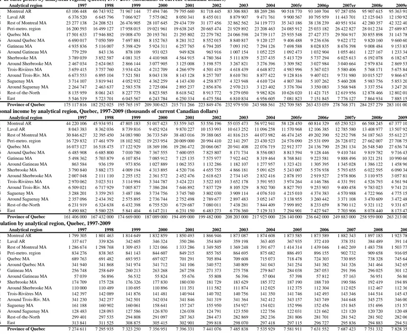
1 100 1 1 1 * 100 1 * 100 0 0 0 0 0 0 N n N n Y y Y y X x X x i t it i t it i t it (II.2.5)Table 1 – GDP at basic prices by analytical region, Quebec, 1997-2009
Relative GDP per cap. Share of population Share of GDP Analytical region 1997 2009 1997 2009 1997 2009
Province = 100 (%) (%) (%) (%)
Montreal and peri-metro area 106 104 -2.5% 58.5% 60.5% 3.3% 62.2% 62.7% 0.8% Montreal MA 113 109 -3.6% 47.1% 48.8% 3.7% 53.0% 52.9% -0.1% 01 Montreal AR 146 137 -5.9% 24.7% 24.6% -0.6% 36.0% 33.7% -6.5% 02 Laval AR 78 86 9.5% 4.6% 5.0% 7.7% 3.6% 4.3% 17.9% 03 Rest of Montreal MA 75 78 3.6% 17.7% 19.2% 8.6% 13.3% 14.9% 12.5% 04 Peri-metro. region 81 84 3.6% 11.5% 11.7% 2.0% 9.3% 9.8% 5.7% Other metropolitan areas 98 104 6.4% 19.6% 19.7% 0.4% 19.2% 20.5% 6.8% Other non-metro 83 84 0.9% 33.4% 31.6% -5.4% 27.8% 26.6% -4.5% Non-metro away from Montreal 85 85 -0.4% 21.9% 19.9% -9.2% 18.6% 16.8% -9.6% Peripheral regions 89 95 6.3% 10.2% 8.9% -12.7% 9.1% 8.5% -7.2% 05 Quebec MA 105 115 9.6% 9.5% 9.5% 0.5% 10.0% 11.0% 10.1% 06 Around Quebec MA 81 78 -4.1% 4.7% 4.4% -6.9% 3.8% 3.4% -10.7% 07 Gatineau MA 80 84 5.3% 3.5% 3.8% 9.0% 2.8% 3.2% 14.7% 08 Around Gatineau MA 57 60 5.7% 0.8% 0.7% -7.4% 0.4% 0.4% -2.1% 09 Sherbrooke MA 90 88 -2.6% 2.4% 2.5% 3.7% 2.2% 2.2% 0.9% 10 Around Sherbrooke MA 93 71 -24.2% 1.5% 1.4% -5.1% 1.4% 1.0% -28.1% 11 Trois-Rivières MA 107 108 1.1% 2.0% 1.9% -5.1% 2.1% 2.0% -4.1% 12 Around Trois-Riv. MA 81 79 -2.9% 4.7% 4.4% -5.8% 3.8% 3.5% -8.5% 13 Saguenay MA 96 107 11.6% 2.2% 1.9% -12.6% 2.1% 2.1% -2.5% 14 Around Saguenay MA 73 75 1.8% 1.8% 1.5% -12.9% 1.3% 1.1% -11.3% 15 Rest-of-the-North 113 126 11.2% 4.1% 3.6% -12.5% 4.6% 4.5% -2.7% 16 East 73 74 0.8% 4.3% 3.8% -12.8% 3.2% 2.8% -12.1% Province of Quebec 100 100 100.0% 100.0% 100.0% 100.0% 1997-2009 proportional change (%) 1997-2009 proportional change (%) 1997-2009 proportional change (%)
It is striking that, without exception, the GDP shares of analytical regions (numbered 01-16 in Table 1) rise or fall according to whether their shares of population rise or fall: the correlation coefficient between the 1997-2009 change in the share of population and the change in the share of GDP is 71% (F-statistic = 14.40)20. A declining relative GDP per capita is also associated with a falling share of GDP: the correlation coefficient between 1997-2009 changes is 72% (F-statistic=15.45). But the change in relative GDP per capita and in the share of population are unrelated: the correlation coefficient is an insignificant 3.2%.
In terms of geographical distribution, what is the picture that emerges? First, population (+3.3%) and, to a lesser degree, production (+0.8%) are concentrating in the Montreal metropolitan and peri-metropolitan area. But the most impressive feature locally is what is happening to the the Montreal AR relative to the rest of the metropolitan and peri-metropolitan area: its share of population has diminished slightly, while its share of GDP has fallen by a substantial 6.5% over a
20
It is readily recognized that, to compare the closeness of relationships, given that the correlation coefficient is a measure of linear dependence, it w ould be mathematically more correct to take the logarithmic transform of equatio n (II.2.4) and compute correlations betw een the logarithm of the left-hand side variable and the logarithms of each of the tw o right-hand side variables. But that w ould make the exposition unnecessarily technical. Given the Maclaurin series ln(1+z)=z–z2/2+z3/3–z4/4+..., w e consider [(xt/x0)–1] to be a first order Taylor approximation of ln(xt/x0) w hen xt is close to x0, so the more correct mathematical approach w ould lead to the same observations.
thirteen-year period. Population and production are being decentralized within the MA and in its vicinity. Outside the Montreal metropolitan and peri-metropolitan area, however, the opposite is happening. All regions but three of the five MAs are losing shares. Of the three MAs gaining shares, two gain heavily in terms of production. Both are administrative cities: Quebec City (+10.1%) is the capital of the Province, and Gatineau (+14.7%) is part of the Ottawa-Gatineau MA, where Canada’s federal capital is located. Everywhere else, population and GDP shares are declining, and they are delining faster in non-metropolitan areas.
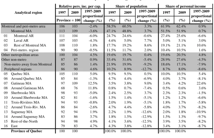
Table 2 presents the same decomposition as Table 1 for personal income. Population data is repeated for readability.
Table 2 – Personal income by analytical region, Quebec, 1997-2009
Relative pers. inc. per cap. Share of population Share of personal income Analytical region 1997 2009 1997 2009 1997 2009
Province = 100 (%) (%) (%) (%)
Montreal and peri-metro area 106 103 -2.4% 58.5% 60.5% 3.3% 61.9% 62.4% 0.9% Montreal MA 113 109 -3.6% 47.1% 48.8% 3.7% 51.5% 51.9% 0.7% 01 Montreal AR 111 104 -6.0% 24.7% 24.6% -0.6% 27.4% 25.6% -6.6% 02 Laval AR 107 103 -4.3% 4.6% 5.0% 7.7% 5.0% 5.1% 3.0% 03 Rest of Montreal MA 108 110 1.8% 17.7% 19.2% 8.6% 19.1% 21.1% 10.6% 04 Peri-metro. region 90 90 -0.5% 11.5% 11.7% 2.0% 10.4% 10.5% 1.6% Other metropolitan areas 100 104 4.5% 19.6% 19.7% 0.4% 19.6% 20.5% 4.8% Other non-metro 87 87 0.9% 33.4% 31.6% -5.4% 28.9% 27.6% -4.5% Non-metro away from Montreal 85 86 1.4% 21.9% 19.9% -9.2% 18.6% 17.1% -7.9% Peripheral regions 86 90 4.6% 10.2% 8.9% -12.7% 8.7% 8.0% -8.6% 05 Quebec MA 105 110 5.0% 9.5% 9.5% 0.5% 10.0% 10.5% 5.4% 06 Around Quebec MA 85 84 -1.3% 4.7% 4.4% -6.9% 4.0% 3.7% -8.1% 07 Gatineau MA 97 109 12.5% 3.5% 3.8% 9.0% 3.4% 4.2% 22.6% 08 Around Gatineau MA 68 76 11.8% 0.8% 0.7% -7.4% 0.5% 0.6% 3.6% 09 Sherbrooke MA 98 93 -5.0% 2.4% 2.5% 3.7% 2.3% 2.3% -1.5% 10 Around Sherbrooke MA 82 81 -1.6% 1.5% 1.4% -5.1% 1.2% 1.2% -6.6% 11 Trois-Rivières MA 94 93 -0.8% 2.0% 1.9% -5.1% 1.8% 1.7% -5.8% 12 Around Trois-Riv. MA 86 84 -2.6% 4.7% 4.4% -5.8% 4.0% 3.7% -8.2% 13 Saguenay MA 92 94 1.9% 2.2% 1.9% -12.6% 2.0% 1.8% -10.9% 14 Around Saguenay MA 83 86 3.7% 1.8% 1.5% -12.9% 1.5% 1.3% -9.7% 15 Rest-of-the-North 94 98 4.9% 4.1% 3.6% -12.5% 3.9% 3.5% -8.2% 16 East 79 83 4.7% 4.3% 3.8% -12.8% 3.4% 3.1% -8.7% Province of Quebec 100 100 100.0% 100.0% 100.0% 100.0% 1997-2009 proportional change (%) 1997-2009 proportional change (%) 1997-2009 proportional change (%)
For personal income as for GDP, analytical regions (numbered 01-16 in Table 2) with declining shares of population also have declining shares of personal income: the correlation coefficient between the 1997-2009 change in the share of population and the change in the share of personal income is 80% (F-statistic = 25.42). But there are a few exceptions (analytical regions 08 and 09). Not surprisingly, the same relationship is observed between the change in GDP and personal income shares: the correlation coefficient between the last column of Table 1 and the last column
of Table 2 is 74% (F-statistic = 17.07). A declining relative personal income per capita is also associated with a falling share of personal income: the correlation coefficient between 1997-2009 changes is 48% (F-statistic = 4.19). But the change in relative personal income per capita and in the share of population are unrelated: the correlation coefficient is a non-significant –14%.
Let us now compare relative personal income per capita in Table 2 with relative GDP per capita in Table 1. The comparison illustrates the conceptual difference between personal income and domestic product. Indeed, personal income is the income that residents of a given territory receive, no matter where production took place; on the other hand, domestic product is the total value of what has been produced in a given territory, no matter where those who receive the income live. Therefore, per capita GDP is strongly influenced by home-to-work commuting. The high per capita GDP of the Montreal AR and, to a lesser degree, of most other MAs is explained by the large number of residents of the surrounding area who come to work there. Conversely, per capita GDP is systematically weaker in the areas around MAs than in the MAs themselves. Two exceptions among the MAs are Gatineau and Sherbrooke. In the case of Gatineau, the somewhat low relative GDP per capita is explained by the fact that Gatineau belongs to the Ottawa-Gatineau MA, and that large numbers of civil servants live in Gatineau and work in Ottawa; indeed, per capita GDP is even lower in the surrounding area. Finally, the high per capita GDP of the Rest-of-the-North region reflects the presence of capital intensive industries (such as mining and hydroelectric power), whose shareholders do not necessarily live there. There is much less variation in relative personal income per capita than in relative GDP per capita, and this results in a less contrasted picture. Nonetheless, it appears that personal income per capita is higher in the Montreal MA, and in the two administrative MAs of Quebec and Gatineau. It should be kept in mind that at least part of that greater personal income is swallowed up by a higher cost of living. Changes in the geographical distribution of personal income reflect both changes in population and changes in per capita personal income, and they are consistent with changes in the distribution of production. There is a slight movement of concentration towards the Montreal metropolitan and peri-metropolitan area, and decentralization within the Montreal MA, with the core Montreal AR losing share. Both administrative capital regions of Quebec and Gatineau increase their shares, and, in the latter case, the increase seems to be spilling over to the surrounding region. All other regions lose share.
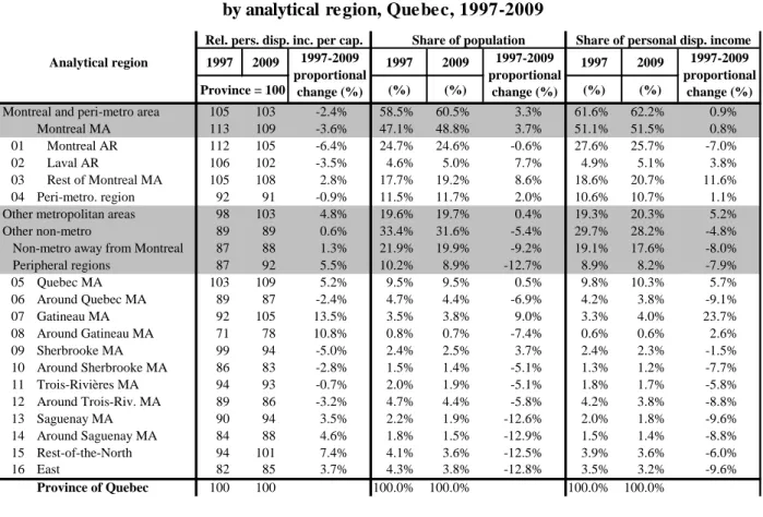
Table 3 presents the same decomposition as Table 1 for disposable personal income. Again, population data is repeated for readability.