This is an author-deposited version published in:
http://oatao.univ-toulouse.fr/
Eprints ID: 9890
To link to this article: DOI: 10.1002/mop.25456
URL:
http://dx.doi.org/10.1002/mop.25456
To cite this version:
Pascaud, Romain and Gillard, Raphaël and Loison,
Renaud On the comparison between multiple-region and dual-grid
finite-difference time-domain methods for the analysis of antenna arrays. (2010)
Microwave and Optical Technology Letters, vol. 52 (n° 10). pp.
2316-2319. ISSN 0895-2477
O
pen
A
rchive
T
oulouse
A
rchive
O
uverte (
OATAO
)
OATAO is an open access repository that collects the work of Toulouse researchers and
makes it freely available over the web where possible.
Any correspondence concerning this service should be sent to the repository
administrator:
[email protected]
ON THE COMPARISON BETWEEN
MULTIPLE-REGION AND DUAL-GRID
FINITE-DIFFERENCE TIME-DOMAIN
METHODS FOR THE ANALYSIS OF
ANTENNA ARRAYS
Romain Pascaud,1Raphae¨l Gillard,2and Renaud Loison2 1De´partement Electronique Optronique et Signal, Institut Supe´rieur de l’Ae´ronautique et de l’Espace, 10 avenue Edouard Belin, Toulouse Cedex 4 31055, France; Corresponding author: [email protected]
2De´partement Antennes et Hyperfre´quences, Institut
d’Electronique et de Te´le´communications de Rennes, 20 avenue des Buttes de Coe¨smes, Rennes Cedex 35043, France
ABSTRACT: A comparison between the multiple-region (MR) and dual-grid (DG) finite-difference time-domain (FDTD) methods for the analysis of antenna arrays is presented. The application of both methods shows that the DG-FDTD method is more accurate when computing the mutual coupling between antennas. Besides, it exhibits multi-surface capabilities that make possible the fast and accurate analysis of antenna arrays, including mutual coupling and edge effects.
Key words: FDTD methods; antenna arrays; antenna array mutual coupling
1. INTRODUCTION
It is well known that the behavior of an isolated antenna differs when it is arranged in an array configuration [1]. Usually, the strongest effects are due to the finite size of the ground-plane and the mutual coupling with adjacent radiating elements. Therefore, the accurate analysis of antenna arrays often requires the numerical modelling of the entire problem.
The finite-difference time-domain (FDTD) method has been successfully used for the analysis of antenna arrays [2]. It allows the characterization of complex heterogeneous 3D struc-tures over a large bandwidth with only one simulation. How-ever, the FDTD method can be inefficient when large problems such as antenna arrays are involved. Indeed, the uniform spatial sampling of the volume generally leads to oversampled areas
that increase the computational time and the memory
requirements.
Several advanced techniques have been proposed to over-come this oversampling problem [2]. Among these solutions, the multiple-region FDTD (MR-FDTD) method [3] has been used to compute the mutual coupling between antennas separated by one wavelength [4]. A MR-FDTD scheme with multiresolution capabilities has also been applied to the analysis of the mutual coupling inside an array of dielectric resonator antennas (DRAs) [5]. Recently, the dual-grid FDTD (DG-FDTD) method has been introduced for the simulation of surrounded antennas [6] and antenna arrays [7].
In this article, we first discuss the limitations of the classi-cal and multiresolution MR-FDTD methods. A comparison between the multiresolution MR-FDTD and the DG-FDTD methods is also carried out for the first time. Finally, the new multi-surface capabilities of the DG-FDTD method are demon-strated and validated on a test case that consists of an array of four DRAs.
2. COMPARISON BETWEEN MR-FDTD AND DG-FDTD METHODS FOR THE ANALYSIS OF MUTUAL COUPLING 2.1. Numerical Methods
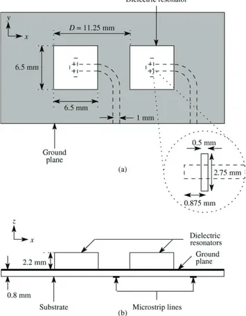
Let us consider the problem shown in Figure 1, where two DRAs are separated by a distanceD.
2.1.1. Multiresolution MR-FDTD Method. With the classical MR-FDTD method, each antenna is described with its own sim-ulation volume, and the two-way communication uses the Kirchhoff near-field to near-field transformation [4]. Thus, the space between the antennas does not have to be meshed, reduc-ing at the same time the numerical dispersion. However, the nu-merical cost of Kirchhoff integrals is usually cumbersome and compression schemes are required [8]. Unfortunately, instability may occur, especially for small distancesD and high compres-sion rates [5]. The easier solution to prevent from instability is to use a one-way communication from the active volume to the passive one, but it does not allow for second-order coupling effects. A MR-FDTD scheme with multiresolution capabilities has been proposed to overcome these instability and inaccuracy problems [5].
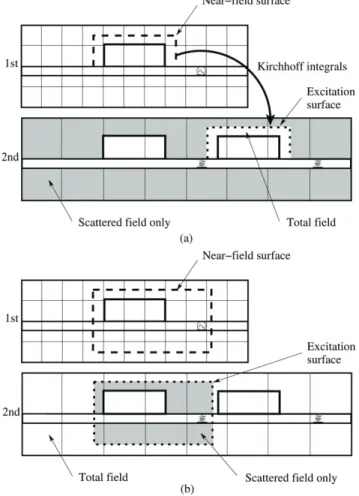
As shown in Figure 2(a), the simulation is now divided into two steps. The first step consists of a fine FDTD simulation of the excited antenna, whereas the second step is a coarse FDTD simulation of the two antennas. During the second step, the gen-erator is switched off since the incident power comes from the Kirchhoff integrals combined with an excitation surface based on the total field/scattered field decomposition principle [2]. The second step should guarantee that the mutual coupling effects are taken into account. However, the use of Kirchhoff integrals implies that the antennas must be separated by free space or placed on an infinite ground-plane. Indeed, in its current form
this transformation does not consider the propagation in hetero-geneous media. As a result, neither the electromagnetic field that propagates inside the dielectric substrate as surface waves, nor the effects due to the finite size of the ground-plane are taken into account.
2.1.2. DG-FDTD Method. The principle of the DG-FDTD
method [7] is relatively close to the multiresolution MR-FDTD one. Both methods successively combine two FDTD simulations with different resolutions. As shown in Figure 2(b), the major difference is that the DG-FDTD method does not use any radia-tion integrals to combine each sub-volume. In fact, it simply modifies the direction of the total field/scattered field decompo-sition and the podecompo-sition of the excitation surface, which is also easier to implement. With such a decomposition, different mate-rials can go through the near-field and excitation surfaces [9]. Moreover, this method is not limited to structures with an infi-nite ground-plane. However, when compared with the MR-FDTD scheme, the DG-MR-FDTD method does not reduce numeri-cal dispersion, but given the small distance between adjacent antennas in an array, this effect is not significant here.
2.2. Example
To compare the multiresolution MR-FDTD and the DG-FDTD methods, we consider the problem presented in Figure 1, where two DRAs are arranged in theE-plane. These DRAs of relative permittivity er¼ 7.8 are placed on an infinite ground-plane and
separated by a distance D ¼ 11.25 mm (about 0.56k0 at 15
GHz). The excitation of each DRA is performed by means of an
aperture in the ground-plane. It has the advantage of having the feeding network below the ground-plane. As shown in Figure 1, microstrip lines printed on a substrate of relative permittivity er
¼ 7.8 are also used.
Three different simulations have been carried out: a multire-solution MR-FDTD, a DG-FDTD, and a classical fine FDTD simulation that is used as a reference. The spatial sampling for the fine resolution isdx ¼ dy ¼ 0.125 mm and dz ¼ 0.1 mm, and the time-step is equal todt ¼ 0.2097 ps. The coarse resolu-tion involves dx ¼ dy ¼ 0.25 mm, dz ¼ 0.2 mm, and dt ¼ 0.419 ps.
The simulated S-parameters are shown in Figure 3. Both advanced methods show a good agreement in theS11parameter
with the reference simulation. Concerning theS21parameter, the
multiresolution MR-FDTD approach suffers from inaccuracies in the lower frequency band, which is not the case with the DG-FDTD method. It can be explained by the fact that the multire-solution MR-FDTD method does not take into account the mu-tual coupling due to surface waves in the substrate. Indeed, it only considers the mutual coupling due to space waves that are dominant at the resonance, but out of the resonance, the surface waves become significant.
Concerning the computational time, both advanced methods exhibit a 1.2 gain when compared with classical FDTD simula-tion. However, larger gains are expected when dealing with larger arrays as will be seen in the next section. Same results are observed for the memory requirements.
3. MULTI-SURFACE CAPABILITIES OF THE DG-FDTD METHOD FOR THE ANALYSIS OF ANTENNA ARRAYS
Most of the time, the principle of pattern multiplication is used to compute the radiation patterns associated with an array of antennas [1]. It simply consists in multiplying the field of a sin-gle radiating element by the array factor that is function of the geometry and the excitation of the array. However, due to the mutual coupling between elements and the finite size of the ground-plane, the radiated far-field might differ from the ideal case. A stringent analysis must therefore be carried out to com-pute the accurate radiated far-field.
As we have seen previously, the DG-FDTD method com-putes with a good accuracy the mutual coupling between ele-ments inside an antenna array, and it also enables the finite size of the ground-plane to be taken into account. But, the DG-Figure 2 Different methods for the simulation of the DRA array: (a)
multiresolution MR-FDTD, (b) DG-FDTD
FDTD method has another interesting feature that is helpful when analyzing antenna arrays. Indeed, as shown in Figure 4, it is possible to put several excitation surfaces during the second step of the DG-FDTD simulation. Each excitation surface is related to an isolated antenna, and its response comes from the first step of the DG-FDTD method. One may notice that for an array of identical sources, only one fine FDTD simulation of the unitary element must be carried out since the excitation surfaces are all the same. The second step of the DG-FDTD method finally gives the radiated far-field by the antenna array while considering mutual coupling and finite ground-plane effects. Furthermore, the amplitude and the phase of the near-field radi-ated by each excitation surface can be modified irrespective of the others, which enable us to test various array configurations.
To illustrate the multi-surface capabilities of the DG-FDTD method, we consider an array of four DRAs arranged in the same configuration as in the example described in Figure 1. The ground-plane has a finite size of 26.5 mm " 60.25 mm (#1.3k0
" 3k0 at 15 GHz). The DG-FDTD results are compared with
the results coming from a classical fine FDTD simulation and the pattern multiplication principle.
3.1. Uniform Amplitude and Phase Excitation
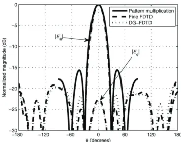
The simplest case is a uniform linear array (ULA) of four DRAs. In that case, all the radiating elements are fed with the same amplitude and phase.
Concerning the DG-FDTD simulation, four excitation surfa-ces are used during the second step. They radiate the near-field coming from the first step, that is to say the isolated antenna response, in phase and with the same amplitude.
The simulated radiated far-fields at 15 GHz in the E plane are presented in Figure 5. The DG-FDTD results fairly match the reference FDTD ones. The pattern multiplication principle shows inaccuracies on the side lobe levels, because it does not account for the environment of the antennas.
3.2. Nonuniform Amplitude Excitation
To reduce the side lobe level, different amplitudes can be applied to each element in the array.
The simulation of such a configuration using the DG-FDTD method is performed by directly weighting each excitation sur-face, that is to say by applying the excitation coefficients on the radiated near-field coming from these excitation surfaces.
In this example, we consider that the amplitude of the excita-tion is equal to 1.0 for the two elements in the center of the array and 0.7 for the two other elements. As we can see in Fig-ure 6, there is a fair agreement between the DG-FDTD and the classical FDTD results, whereas the pattern multiplication prin-ciple is still inaccurate.
3.3. Nonuniform Phase Excitation
It is well known that modifying each phase element individually leads to a scan of the main beam.
With the DG-FDTD method, the phase shifting is performed by delaying each excitation surface in the time domain, which is equivalent to true time-delay phase shifting. Thus, if we know the phase shift a between the excitations of the array at a fre-quency pointf0, we can compute the equivalent time delay
tdelay¼ a 2pf0:
(1)
On the other hand, if a particular scanning angle y0is required,
the associated time delay is given by
tdelay¼d sin h
c : (2)
In this example, the scanning angle y0 is equal to 30$, which
implies a time delaytdelay between each excitation of 18.75 ps.
Figure 7 presents the simulated radiated far-fields at 15 GHz. We notice a slight change in the scanning angle when Figure 4 Multi-surface capabilities of the DG-FDTD method
Figure 5 Antenna array normalized radiated far-field at 15 GHz in the (x-z) plane: uniform amplitude and phase excitation
Figure 6 Antenna array normalized radiated far-field at 15 GHz in the (x-z) plane: nonuniform amplitude excitation
considering the real array geometry. Same comments can be made concerning the accuracy of the DG-FDTD method. 3.4. Computational Time and Memory Requirements
The overall simulation of these three configurations takes 8 h and 45 min using a classical FDTD code. The three DG-FDTD simulations take 1 h and 27 min, that is to say a reduction in computation time by a factor of 6.0. In fact, the first step takes 30 min and each coarse FDTD simulation associated with the second step takes 19 min.
Concerning the memory requirements, the classical fine FDTD simulation needs 762 Mb. For the DG-FDTD method, the maximum memory occupation appears during the second step and it is equal to 200 Mb, that is to say a reduction in memory requirements by a factor of 3.8.
4. CONCLUSIONS
A comparison between the multiresolution MR-FDTD and the DG-FDTD methods for the mutual coupling analysis in antenna arrays has been presented. The DG-FDTD turns out to be more accurate and easier to implement since it does not use any radiation integrals. Moreover, the multi-surface capabilities of the DG-FDTD method make it very attractive for the fast analysis of antenna arrays. REFERENCES
1. R.J. Mailloux, Phased array antenna handbook, 2nd ed., Artech House, Norwood, MA, 2005.
2. A. Taflove and S.C. Hagness, Computational electrodynamics: The finite-difference time-domain method, 3rd ed., Artech House, Nor-wood, MA, 2005.
3. J.M. Johnson and Y. Rahmat-Samii, MR/FDTD: A multiple-region finite-difference time-domain method, Microwave Opt Technol Lett 14 (1997), 101–105.
4. A.J. Parfitt and T.S. Bird, Computation of aperture antenna mutual coupling using FDTD and Kirchhoff field transformation, Electron Lett 34 (1998), 1167–1168.
5. A. Laisne´, R. Gillard, and G. Piton, New multiple-region schemes with multiresolution capabilities for the FDTD analysis of radiating structures, Microwave Opt Technol Lett 33 (2002), 268–273. 6. R. Pascaud, R. Gillard, R. Loison, J. Wiart, and M.-F. Wong,
Dual-grid finite-difference time-domain scheme for the fast simula-tion of surrounded antennas, IET Microwave Antennas Propag 1 (2007), 700–706.
7. R. Pascaud, R. Gillard, R. Loison, J. Wiart, M.-F. Wong, B. Lind-mark, and L. Garcia-Garcia, New DG-FDTD method: Application to the study of a MIMO array, In: IEEE AP-S International Sym-posium on Antennas and Propagation, Honolulu, HI, 2007, pp. 3069–3072.
8. A. Laisne´, R. Gillard, and G. Piton, A new multiresolution near-field to near-near-field transform suitable for multi-region FDTD schemes, In: IEEE MTT-S International Microwave Symposium, Phoenix, AZ, 2001, pp. 893–896.
9. R. Pascaud, R. Gillard, R. Loison, J. Wiart, and M.-F. Wong, Ex-posure assessment using the dual-grid finite-difference time-domain method, IEEE Microwave Wireless Compon Lett 18 (2008), 656–658.
VC2010 Wiley Periodicals, Inc.
MEASUREMENT OF STOKES
PARAMETERS OF TERAHERTZ
RADIATION IN TERAHERTZ
TIME-DOMAIN SPECTROSCOPY
Hui Dong,1Yandong Gong,1and Malini Olivo2,3,4
1Institute for Infocomm Research, 1 Fusionopolis Way, #21-01 Connexis, Singapore 138632, Singapore; Corresponding author: [email protected]
2
National Cancer Center, 11 Hospital Drive, Singapore 169610, Singapore
3
Singapore Bioimaging Consortium, Biomedical Sciences Institutes, 11 Biopolis Way, #02-02 Helios, Singapore 138667, Singapore
4School of Physics, National University Ireland, Galway, Ireland
Received 6 January 2010
ABSTRACT: We propose a technique for the measurement of Stokes parameters of terahertz radiation in terahertz time-domain spectroscopy (THz-TDS). In this technique, a rotatable wire-grid THz polarizer is placed in front of a two-contact photoconductive THz detector. Stokes parameters can be measured by making two temporal scans corresponding to two angles of the polarizer. We theoretically demonstrate that the two angles can be %45$and 45$for achieving the
statistically best measurement accuracy in a single test.VC 2010 Wiley Periodicals, Inc. Microwave Opt Technol Lett 52:2319–2324, 2010; Published online in Wiley InterScience (www.interscience.wiley.com). DOI 10.1002/mop.25450
Key words: terahertz time-domain spectroscopy; state of polarization; Stokes parameters
1. INTRODUCTION
Terahertz time-domain spectroscopy (THz-TDS) is a very useful and powerful technique for measuring the optical properties of many materials in the frequency range from a few tens of giga-hertz to a few teragiga-hertz. The refractive index and attenuation coefficient of a material are usually detected in THz-TDS [1]. In addition to these two optical parameters, polarization properties of some materials in THz frequency range attract more and more attentions [2]. To detect the polarization properties of a material using THz-TDS, first of all, the state of polarization (SOP) of the THz radiation must be measured in THz-TDS. With some combinations of measured input and output SOPs, the polarization properties of the material under test can be obtained [3]. It is well known that the SOP of an electromag-netic wave can be depicted by Jones vector or Stokes parame-ters. Because THz radiation in THz-TDS is completely coherent (so the Fourier transform of the time domain THz electric field can be performed), Jones vector and Stokes parameters can be Figure 7 Antenna array normalized radiated far-field at 15 GHz in the