Bifurcation analysis of a periodically forced relaxation oscillator:
Differential model versus phase-resetting map
H. Croisier,1,
*
M. R. Guevara,2and P. C. Dauby1 1Institut de Physique B5a, Université de Liège, Allée du 6 Août 17, 4000 Liège, Belgium 2
Department of Physiology and Centre for Nonlinear Dynamics in Physiology and Medicine, McGill University, 3655 Sir William Osler Promenade, Montreal, Quebec, Canada H3G 1Y6
共Received 20 June 2008; published 20 January 2009兲
We compare the dynamics of the periodically forced FitzHugh-Nagumo oscillator in its relaxation regime to that of a one-dimensional discrete map of the circle derived from the phase-resetting response of this oscillator 共the “phase-resetting map”兲. The forcing is a periodic train of Gaussian-shaped pulses, with the width of the pulses much shorter than the intrinsic period of the oscillator. Using numerical continuation techniques, we compute bifurcation diagrams for the periodic solutions of the full differential equations, with the stimulation period being the bifurcation parameter. The period-1 solutions, which belong either to isolated loops or to an everywhere-unstable branch in the bifurcation diagram at sufficiently small stimulation amplitudes, merge together to form a single branch at larger stimulation amplitudes. As a consequence of the fast-slow nature of the oscillator, this merging occurs at virtually the same stimulation amplitude for all the period-1 loops. Again using continuation, we show that this stimulation amplitude corresponds, in the circle map, to a change of topological degree from one to zero. We explain the origin of this coincidence, and also discuss the transla-tional symmetry properties of the bifurcation diagram.
DOI:10.1103/PhysRevE.79.016209 PACS number共s兲: 05.45.Xt, 87.19.ln, 87.19.Hh
I. INTRODUCTION
Biological systems that oscillate can often be modeled as relaxation oscillators, in which the state point of the system moves relatively slowly within two well-separated regions of the phase space 共the slow or “relaxation” phases of the os-cillation兲, with much faster jumps between these two regions 关1,2兴. The FitzHugh-Nagumo 共FHN兲 model is a simple
two-variable model of an excitable cell, in which excitability is intimately linked with the fast-slow nature of the trajectories 关3兴. Indeed, it can be easily turned into a relaxation oscillator
by changing a single parameter away from its nominal value 关3兴. This is not at all surprising, given that the original
excit-able FHN system came from the van der Pol oscillator, modi-fied so as to remove the limit-cycle oscillation but maintain excitability关4兴: hence the original name given to these
equa-tions by FitzHugh, the Bonhoeffer–van der Pol equaequa-tions关3兴.
Biological oscillators are in turn themselves typically sub-ject to external periodic forcing 关5兴. There have been many
studies on the periodically forced FHN oscillator 共e.g., 关6–11兴兲, as well as on the periodically forced van der Pol
oscillator共e.g., see 关12兴 for a review; 关2,13,14兴兲. These have
yielded a plethora of rhythms, including periodic 共“phase-locked”兲, quasiperiodic, and chaotic rhythms. Similar behav-iors are seen in low-dimensional nonrelaxation oscillators 关13–37兴, and in low-dimensional fast-slow excitable systems
关10,11,30,38–48兴.
In order to gain insight into the extremely complicated response to periodic stimulation, the usual practice of carry-ing out direct numerical integration of the full equations is insufficient. Two additional approaches have been employed in the literature. The first one uses numerical continuation
methods, coupled with algorithms to identify bifurcations, to study the periodic solutions of the full differential equations 共or, equivalently, to study the fixed points of the stroboscopic maps of the system兲. While such methods have been used many times to study forced oscillators in their nonrelaxation regime 关17,18,21–25,29,31–33,35–37兴, and, to a lesser
ex-tent, forced fast-slow excitable systems 关39,48兴, they have
been applied only rarely to forced oscillators in the relax-ation regime 共e.g., 关13兴兲.
The second approach involves some degree of approxima-tion, in that one reduces consideration of the forced two-dimensional system to analysis of a one-two-dimensional discrete map, for which the numerical computations are easier, and for which one can occasionally even obtain analytic solu-tions. This has been carried out in two ways. In the first way, one assumes the singular limit, so that the motion of the unforced oscillator is essentially one dimensional, with the state point of the system moving on the two stable sheets of the critical manifold except for instantaneous jumps between these two sheets关2,14,44–46,49–51兴. In the second way, one
first characterizes the phase-resetting response of the oscilla-tor to a single stimulus pulse delivered systematically at vari-ous phases throughout its cycle. Then, assuming that there is a sufficiently fast return of the trajectory back to the limit cycle, one derives a one-dimensional circle map共the phase-resetting map兲 that can then be iterated to predict the re-sponse to periodic stimulation共e.g., 关6,10,19,52–55兴兲. A
one-dimensional return map has sometimes also been obtained by measuring the phases of the cycle at which successive stimuli arrive during periodic stimulation 共e.g., 关8,54,56兴兲.
It is known that an important topological feature of these one-dimensional circle maps, namely, their topological degree, changes with stimulation amplitude 共e.g., 关9,19,26,54,55,57–59兴兲 and that this topological degree
con-strains the classes of rhythms that can be seen 共e.g., 关60兴兲.
In this paper, we show that the topological degree of the phase-resetting map of a relaxation oscillator changes from one to zero at the same stimulation amplitude as that at which the period-1 loops in the bifurcation diagram of the full differential equations merge with an everywhere-unstable period-1 branch. We explain this coincidence by the fact that the bifurcation diagram of any circle map where the bifurcation parameter 共in our case, the stimulation period兲 appears only in an additive fashion has its period-1 fixed points belonging to isolated loops when the topological de-gree of the map is one, while these fixed points belong to a unique branch when the topological degree of the map is zero. Therefore, if the phase-resetting map is a good approxi-mation of the full differential equations, it must change to-pological degree for the same stimulation amplitude as that at which the merging of period-1 solution branches occurs in the bifurcation diagram of the original equations. To our knowledge, this is the first time that this property of circle maps has been underscored. We also discuss the extent to which the translational symmetry that characterizes the bifur-cation diagram of circle maps 关19,61兴 holds in the
bifurca-tion diagram of the differential equabifurca-tions.
The paper is organized as follows. In Sec.II, we perform a continuation analysis of the differential model, which is a forced FHN oscillator in its relaxation regime, using the stimulation period as bifurcation parameter. We study how the bifurcation diagram evolves as the stimulation amplitude is raised. In particular, we note that the merging of the period-1 loops with the everywhere-unstable branch of the same period occurs at virtually the same amplitude for all loops. In Sec.III, we investigate how well this evolution is accounted for by the phase-resetting map. We use a graphical method to obtain the period-1 fixed points of the map, which allows us to deduce the topological property of circle maps announced above. We then take advantage of the transla-tional invariance of the bifurcation diagram of circle maps 关19,61兴 in order to compare the period-M bifurcation points
of the map to those of the differential equations. Finally, in Sec.IV, we put our results into perspective with prior related works.
II. DIFFERENTIAL MODEL OF THE FORCED RELAXATION OSCILLATOR
A. Equations and numerical methods We study the periodically forced FHN oscillator:
du
dt = Au共1 − u兲共u − us兲 − v + I共t兲, dv
dt =共u − cv − d兲, 共1兲
where A = 1, us= 0.2, c = 0.4, d = 0.2, and =0.005. The
pa-rameter values are such that the unforced system 关I共t兲=0兴 possesses a globally attracting limit cycle, enclosing an un-stable node. The period of the limit cycle is T0= 165.191. If one thinks of Eq. 共1兲 as being a reduced form of the
Hodgkin-Huxley model, then the variable u corresponds to
the electrical potential across the cell membrane while the variablev is a slow “gating” variable. The difference of time scale between the two variables, which is characteristic of relaxation oscillations, is produced by the smallness of .
The periodic stimulation I共t兲 is a train of Gaussian-shaped pulses:
I共t兲 = I0
兺
j=−⬁ ⬁
exp关− 共t − jT兲2/2兴, 共2兲 where I0 is the stimulation amplitude, T is the stimulation period, and = 1. This choice of ⰆT0 guarantees that the stimulus is effectively “on” during a time much shorter than the intrinsic period of the oscillator, since the Gaussian func-tion, although never zero, is rapidly decreasing.
We used the method described in 关48兴 in order to follow
periodic solutions of 共1兲–共2兲withAUTO97 continuation soft-ware关62兴 共see also the discussion in Sec.IVbelow兲.
B. Theoretical background
Before describing our numerical results, let us summarize a few theoretical results about periodically forced planar os-cillators, under the hypothesis that the unforced oscillator is described by a globally attracting limit cycle of period T0 enclosing an unstable fixed point 共see also 关23,31,32,63兴兲.
The extended phase space of the forced oscillator is R2 ⫻S1, since the unforced oscillator is two-dimensional共2D兲 and since the forcing is a periodic function of time unaf-fected by the oscillator, allowing the time to be considered modulo the共normalized兲 stimulation period T/T0.
At zero stimulation amplitude, and for any value of T/T0, the extended phase space contains a globally attracting in-variant two-torus, given by the product of the globally at-tracting limit cycle of the unforced system byS1, which de-scribes the forcing, and an unstable limit cycle of period 1, enclosed within the torus, given by the product of the un-stable fixed point of the unforced system byS1. The globally attracting character of the invariant torus means that all at-tractors must lie on the torus, although the torus may not be an attractor itself共see, e.g., 关64兴, Chap. 1兲.
For sufficiently small stimulation amplitude, both the in-variant torus and the unstable limit cycle enclosed by the torus are guaranteed to persist, because they are “normally hyperbolic” invariant manifolds at zero stimulation ampli-tude关65,66兴. 共An invariant manifold is normally hyperbolic
if, under the dynamics linearized about the invariant mani-fold, the growth rate of vectors transverse to the manifold dominates the growth rate of vectors tangent to the manifold 关66兴.兲 The normal hyperbolicity of the torus is a consequence
of the hyperbolicity of the attracting limit cycle of the forced equations, while the normal hyperbolicity of the un-stable limit cycle enclosed by the torus is a consequence of the hyperbolicity of the repelling fixed point of the unforced equations. With the exception of the unstable limit cycle en-closed by the torus, no hyperbolic solution can exist outside of the globally attracting torus at small forcing amplitude, because it would then have to exist at zero amplitude, while by assumption no such orbit exists for I0= 0. Hence, for I0
sufficiently small, the asymptotic dynamics is essentially re-stricted to the invariant torus, and this constrains substan-tially the types of behavior that can occur. In particular, the existence of a globally attracting invariant torus for the dif-ferential equations is equivalent to the existence of a globally attracting invariant circle for the “stroboscopic maps” of the system 共the 2D discrete maps obtained by stroboscopically sampling the flow at time intervals equal to the forcing pe-riod兲. This implies that the study of the forced oscillator essentially reduces to that of a family of discrete maps of the circle. These circle maps are, moreover, invertible since the stroboscopic maps of differential flows are invertible maps of the plane. Many important properties have been proved for such invertible circle maps 共e.g., 关67–69兴兲, some of which
we enunciate now in terms of the invariant torus of the dif-ferential equations.
A rotation number can be associated with every solution on the torus. Geometrically, it corresponds to the average number of times the solution winds around the meridian of the torus per forcing period. When the rotation number is rational, the solution is periodic; when it is irrational, the solution is quasiperiodic, with the trajectory densely cover-ing the torus. The rotation number is unique for a given value of 共T/T0, I0兲, which implies that the coexistence of periodic solutions of different period, as well as the coexistence of periodic and quasiperiodic motions, is forbidden on the torus 共this would indeed imply the intersection of the trajectories兲. A stable periodic solution never exists alone on the torus, but is always paired with an unstable solution of the same pe-riod, with the stable solution being a nodal limit cycle, and the unstable one being a saddle limit cycle. The region in the 共T/T0, I0兲 parameter plane where a periodic solution with period MT and rotation number N/M exists is called an N/M Arnol’d tongue, or N/M resonance horn, or M :N phase-locking zone 共M ,N integers兲. Each N/M Arnol’d tongue originates from the point T/T0= N/M on the T/T0 axis and generically opens up into the upper half of the parameter plane as a “wedge”共i.e., the two sides of the tongue are not tangent to one another at zero amplitude兲, bounded by saddle-node bifurcation curves.
At larger stimulation amplitudes, the invariant torus is no longer guaranteed to persist, and indeed typically breaks up. The aforementioned results then no longer hold and one has to revert to studying the full differential equations, or the associated stroboscopic maps of the plane. Although some general results do exist about the latter 共e.g., 关32兴兲, the
dy-namics of such systems is much less constrained than that of circle maps, so that numerical continuation is often needed to study the details of the wealth of phenomena that can occur.
C. Results
We have computed bifurcation diagrams with the stimu-lation period T as bifurcation parameter, the stimustimu-lation am-plitude I0 being fixed, restricting our analysis to periodic solutions of period P = MT 共or period-M solutions兲 with M 艋3. The stimulation period T was kept above Tmin⯝10, in order to avoid substantial overlap of successive stimuli, and below some Tmaxwhich depends on the bifurcation diagram, but chosen large enough so that the 1:2 rhythm is computed in each case共2.25T0⬍Tmax⬍3T0兲. In all the bifurcation dia-grams that follow, black curves represent stable solutions, gray curves represent unstable solutions, black crosses are saddle-node共SN兲 bifurcations, and purple circles are period-doubling 共PD兲 bifurcations. The normalized stimulation pe-riod T/T0 is plotted along the abscissa. The L2-norm of the solutions, that is,兵共1/ P兲兰0P关u2共t兲+v2共t兲兴dt其1/2, where P is the period of the solution, is plotted along the ordinate. The “M : N” labels indicate the phase-locked rhythms to which the period-M solutions correspond 共“phase-locked rhythm” is used in this paper indifferently from “periodic solution,” with no implication about the stability of the solution兲. The way these labels are assigned is discussed at the end of this section. We now describe the evolution of the bifurcation diagram as I0 is increased.
For very small stimulation amplitudes, e.g., I0= 0.1共Fig.
1兲, all stable periodic solutions belong to isolated closed
loops in the bifurcation diagram. The only bifurcation points on these loops are saddle-nodes, which is consistent with the persistence of the invariant torus. Most loops in Fig.1
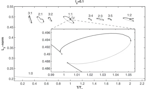
con-0.2 0.4 0.6 0.8 1 1.2 1.4 1.6 1.8 2 2.2 0.2 0.25 0.3 0.35 0.4 0.45 0.5 0.55 T/T 0 L 2 −norm I 0=0.1 3:1 2:1 3:2 1:1 3:4 2:3 3:5 1:2 1:0 0.99 1 1.01 1.02 1.03 1.04 1.05 0.486 0.488 0.49 0.492 0.494 0.496
FIG. 1. Bifurcation diagram computed with AUTO for I0= 0.1. Black curves indicate stable solu-tions; gray curves indicate un-stable solutions. The only bifurca-tions present are saddle-nodes 共⫻兲. The zoom on part of the 1:1 loop shows two of the three pairs of SNs on that loop, which give rise to 1 : 1↔1:1 bistability 共1:1 self-bistability兲 in two ranges of T/T0.
tain only two saddle-nodes, where the stable-unstable pairs of solutions meet, and which define their boundaries with respect to T/T0 共and thus give the edges of the Arnol’d tongue in cross section at that I0兲. The period-1 loops, how-ever, contain three pairs of saddle-nodes, which gives rise to regions of bistability. The zoom in Fig.1, for instance, shows that there are two ranges of T/T0over which there is coex-istence of two stable 1:1 rhythms 共0.9971⬍T/T0⬍0.9983 and 1.003⬍T/T0⬍1.052兲, which we term 1:1 “self-bistability.” Figure2shows one of these pairs of bistable 1:1 rhythms. Continuation of the period-1 saddle-nodes in the two-parameter共T/T0, I0兲 plane shows that the bistability ex-ists all the way down to zero amplitude 共Fig.6兲. This does
not contradict the persistence of the globally attracting torus mentioned earlier since these solutions have the same period. In fact, the occurrence of such self-bistability at arbitrarily small stimulation amplitudes has been shown to be a generic feature of periodically forced planar oscillators共see 关70兴 and
the discussion in Sec. IV D兲. The regions in the
two-parameter plane which are bounded by the “secondary” SN curves in Fig.6共dashed and dotted curves兲 have been termed
Arnol’d flames关63,70兴.
In addition to the isolated loops, the bifurcation diagram at small I0 contains an everywhere-unstable period-1 branch 共bottom branch in Fig. 1兲. This branch reflects the
persis-tence at finite I0 of the unstable limit cycle existing in the extended phase space at zero amplitude. Projection of solu-tions from this branch on the 共u,v兲 phase plane shows that the state point indeed remains in the vicinity of the unstable node of the unforced system, passing closer and closer to it as the stimulation period increases共Fig.3兲. These solutions
are reminiscent of canards, in that a segment of the trajectory remains close to the middle branch of the u-nullcline, which constitutes the unstable part of the critical manifold of the unforced equations共the critical manifold of a fast-slow sys-tem is the nullcline associated with the fast variable; see, e.g., 关71兴兲. The standard rotation number is not defined for
these solutions since, for each given value of T/T0, the so-lution does not lie on the invariant torus but constitutes the unstable limit cycle enclosed by the torus. However, if one uses the “physiological” definition that an M : N rhythm is a
period-M response in which N action potentials are elicited, these solutions have to be called 1:0 rhythms, because the period-1 response is of too small an amplitude to be consid-ered an action potential共AP兲. Indeed, in the FHN model, an AP is notably characterized by the state point visiting the vicinity of the right branch of the u-nullcline关as is the case, e.g., in the phase-plane trajectories in Fig.2共b兲兴.
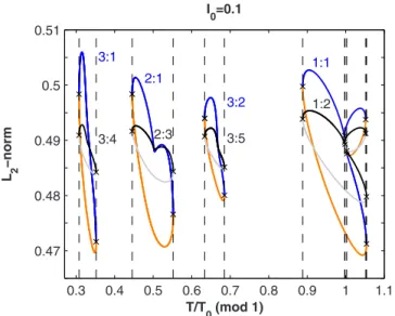
Another characteristic of Fig. 1is the approximate trans-lational invariance of the bifurcation diagram. If the loops to the right of the 1:1 rhythm are shifted left by an amount T/T0= 1, then each M : N loop for T/T0⬎1.2 is paired with an M : N − M loop for T/T0⬍1.2, and the locations of the saddle-nodes on each pair of loops virtually coincide 共Fig.
4兲. We shall return to consider this symmetry further later on
共Sec. III B 5兲.
At a higher value of I0, pairs of period-doubling points appear on the isolated loops. They are present, e.g., for I0 = 0.133 共Fig. 5兲. In the ranges of T/T0 where a
period-0 0.5 1 −0.4 0 0.5 1 t/T0 u −0.2 0.2 0.6 1 −0.02 0.02 0.06 0.1 0.14 u v (a) (b)
FIG. 2. The pair of bistable 1:1 rhythms existing at I0= 0.1, T/T0= 1.03.共a兲 u共t兲 plotted over one period. 共b兲 projection of the solutions on the共u,v兲 phase plane 共solid curves兲. The trajectories are traveled counterclockwise. Dashed curves give the nullclines of the unforced system. −0.05 0 0.05 0.1 0.15 0.2 0.25 −0.01 −0.005 0 0.005 0.01 u v
FIG. 3. Projections onto the共u,v兲 phase plane of solutions be-longing to the unstable 1:0 branch for I0= 0.1, obtained usingAUTO. The unstable fixed point of the unforced system lies at the intersec-tion of the nullclines 共dashed curves兲. T/T0 varies from 0.234 共lightest gray curve兲 to 2.46 共black curve兲.
doubled solution is born, the invariant torus can no longer exist. Indeed, for a given value of T/T0, the period-doubled solution cannot lie on the invariant torus because it would intersect the periodic solution from which it originates. Nei-ther can it lie outside of this torus because this would imply a crossing of the invariant torus by the period-doubled solu-tion.
One of the points from each PD pair is very close to the rightmost SN of each loop共e.g., at point C in Fig.5兲, so that
the two different bifurcations look like they are occurring at the same point in the figure. On some loops, the right PD point was not even identified by AUTO. This is because the continuation step used in these computations was not small enough to detect the two consecutive bifurcations 共SN-PD兲. We have performed a two-parameter continuation of the left PD point for some loops and in each case, the PD bifurcation curve leads to the right PD point, as shown in Fig.6for the 1:1 loop. Figure6also shows that the proximity of the right-most SN and PD points actually persists over a large range of parameters values, since the bottom part of the PD branch 共thick purple curve兲 is indistinguishable from the nearest SN branch 共solid black curve兲. The two bifurcation curves be-come more separated from each other as larger values of are used, and so we believe that their close proximity in Fig.
6 is related to the nearly singular nature of the system 关 Ⰶ1 in Eq. 共1兲兴. The fact that the two bifurcation curves
ex-tend greatly to the right共they actually extend further than the right limit of Fig.6兲, in a quasihorizontal manner, is also due
to the smallness of.
The two PD points of each pair 共e.g., A and C in Fig.5兲
are connected by a branch of period-2 solutions. However, for the sake of clarity, we show in Fig.5the period-2 branch only for the 1:1 loop, and use a different color scheme to indicate its stability 共blue for stable solutions, orange for unstable solutions兲 to distinguish this branch from the period-1 branch. This period-2 branch is unstable for most of the range of T/T0 values over which it exists, as the domi-nant orange 共gray兲 color indicates. A stable 2:2 rhythm is, however, present in the tiny region between point A 共PD of period-1 solution兲 and point B 共PD of period-2 solution兲. The
0.3 0.4 0.5 0.6 0.7 0.8 0.9 1 1.1 0.47 0.48 0.49 0.5 0.51 T/T0(mod 1) L 2 −norm I0=0.1 3:1 3:4 2:1 2:3 3:2 3:5 1:1 1:2
FIG. 4. 共Color online兲 Illustration of the approximate transla-tional symmetry of the bifurcation diagram for I0= 0.1. The loops to the right of the 1:1 rhythm are shifted left by an amount T/T0= 1. For the unshifted loops, blue indicates stable solutions, orange in-dicates unstable solutions. The locations of the SNs for the shifted loops are highlighted by vertical dashed lines, to allow comparison with the corresponding bifurcations for the unshifted loops.
0.4 0.6 0.8 1 1.2 1.4 1.6 1.8 2 2.2 2.4 0.2 0.22 0.4 0.42 0.44 0.46 0.48 0.5 0.52 L 2 −norm I0=0.133 3:1 2:1 3:2 1:1 3:4 2:3 3:5 1:2 T/T0 1:0 A B C
FIG. 5.共Color online兲 Bifurcation diagram for I0= 0.133. Pairs of PD points共䊊兲 have appeared on the loops, with the rightmost PD point of each pair being very close to a SN共⫻兲, as at point C. The rightmost PD point has sometimes been missed by the computation 共cf. text兲. The period-2 branch that connects each pair of PD points is shown only for the 1:1 loop. It is stable in the tiny region between point A and point B共blue color兲 and unstable virtually everywhere between point B and point C 共orange color兲. The PD point A belongs to the period-1 branch while the PD point B belongs to the period-2 branch. Note the y-axis break.
two PD points A and B might thus be the first two members of a supercritical period-doubling cascade that produces period-doubled phase-locking zones within the Arnol’d tongues, and which can even progress to chaotic dynamics 共e.g., 关17,29兴兲.
If the amplitude is raised just a little further, a spectacular change occurs in the bifurcation diagram: the period-1 loops merge with the everywhere-unstable period-1 branch, and the
period-2 loops merge with period-2 branches that have grown out of the everywhere-unstable period-1 branch via the birth of pairs of PD points. For instance, for I0= 0.135 in Fig.7, both the 1:1 loop and the 1:2 loop have merged with the 1:0 branch, the 2:3 loop has merged with a period-2 branch emanating from the period-1 branch, and the 2:1 loop is close to undergoing the same process as the 2:3 loop with another period-2 branch that has grown below the 2:1 loop.
0.5 1 1.5 2 2.5 0 0.1 0.2 0.3 0.4 0.5 0.6 0.7 0.8 T/T0 I 0 0.950 1 1.05 1.1 0.05 0.1 0.15 SN SN SN PD A C
FIG. 6. 共Color online兲 Loci of the three pairs of SNs 共thin solid, dashed, and dotted black curves兲 and of the pair of PDs 共thick purple curve兲 on the 1:1 loop. The zoom shown in the inset allows the two SNs belonging to the narrowest locus 共dotted curve兲 to be distinguished from each other. Points A and C are those from Fig.5.
0.5 1 1.5 2 2.5 3 0.2 0.25 0.3 0.35 0.4 0.45 0.5 0.55 T/T0 L 2 −norm I0=0.135 (I0=0.133) 3:1 2:1 3:2 1:1 3:4 2:3 3:5 1:2 1:0
FIG. 7. 共Color online兲 Bifurcation diagram for I0= 0.135. The unstable segments of the 3:4 and 3:5 loops are drawn in orange, in order to facilitate their identification. The dotted curves in the background repeat the bifurcation diagram for I0= 0.133共disregarding stability兲, in order to underline the huge qualitative change that has occurred. Note how the 2:1 loop is about to merge with the period-2 branch immediately below it.
We were not able to determine numerically which of the period-1 loops merges first with the unstable period-1 branch: we find that all merge for I0= Ith= 0.1338⫾0.0001. We are convinced that this very delicate behavior is related again to the nearly singular nature of the system, since the successive mergings can be distinguished if a larger value of is used 共e.g., using =0.02 and = 0.25兲. It should be noted that the 3:4 and 3:5 solutions, like the 3:1 and 3:2 solutions, still form closed loops for I0⬎Ith. But because the unstable parts of these loops pass very close to the period-1 and period-2 branches, this is not easy to realize at first sight 共we have used orange in Fig. 7 to highlight the unstable segments of the period-3 loops兲. The crossings of the 3:4 and 3:5 loops with the 2:3 loop are only apparent 共two different solutions can have the same L2-norm兲. The rightmost SN on the 3:5 loop is very close to a SN on the period-1 branch, and remains so over a finite range of stimulation amplitude. This
characteristic is yet again due to the use of a small value of . Finally, the dotted gray curves in the background of Fig.7
superimpose the bifurcation diagram for I0= 0.133 共disre-garding stability兲, in order to underscore the huge change that has occurred in the qualitative picture following the minute change of amplitude from I0= 0.133 to 0.135.
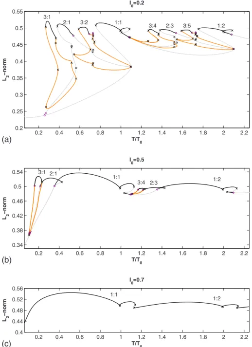
For I0= 0.2关Fig.8共a兲兴, the 2:1 loop has merged with the
period-2 branch below it. The 3:2 loop, in a fashion similar to the 3:5 loop, now has its rightmost SN virtually touching the period-1 branch.
For I0= 0.5关Fig. 8共b兲兴, we no longer find stable 3:2 and 3:5 rhythms. Instead, 2 : 1↔1:1 bistability and 2:3↔1:2 bistability are seen. 3 : 1↔2:1 bistability and 3:4↔2:3 bi-stability are also present.
For I0= 0.7关Fig.8共c兲兴, only the period-1 branch remains. All the period-doubled branches have disappeared through collision and annihilation of the PD points on each branch.
0.2 0.4 0.6 0.8 1 1.2 1.4 1.6 1.8 2 2.2 0.2 0.25 0.3 0.35 0.4 0.45 0.5 0.55 T/T0 L 2 −norm I0=0.2 3:1 2:1 3:2 1:1 3:4 2:3 3:5 1:2 0.2 0.4 0.6 0.8 1 1.2 1.4 1.6 1.8 2 2.2 0.34 0.38 0.42 0.46 0.5 0.54 T/T0 L 2 −norm I0=0.5 3:1 2:1 1:1 3:4 2:3 1:2 0.2 0.4 0.6 0.8 1 1.2 1.4 1.6 1.8 2 2.2 0.4 0.44 0.48 0.52 0.56 T/T0 L 2 −norm I0=0.7 1:1 1:2
(a)
(b)
(c)
FIG. 8.共Color online兲 Bifurca-tion diagrams for I0= 0.2, 0.5, and 0.7. The unstable portions of the period-3 loops are drawn in orange.
All the loops have also disappeared, and it is likely that the period-1 branch is truly the only periodic solution left, since the external forcing is expected to dominate the dynamics of the system at very large stimulation amplitudes, as in several other models of periodically forced oscillators 关20,23,29–34,63兴. One of the two pairs of saddle-nodes still
present on the 1:1 branch for I0= 0.7 共the rightmost pair兲 disappears at slightly larger stimulation amplitudes 共I0 = 0.782兲, as can be seen from the closing of the dashed curve in Fig. 6. The remaining pair共dotted curve in Fig.6兲
disap-pears only at a huge stimulation amplitude共I0= 155兲. Before closing this section, let us discuss briefly how we have labeled the M : N rhythms in the bifurcation diagrams. With the exception of the everywhere-unstable period-1 branch existing at small I0, we have labeled only the stable portions of branches. At small stimulation amplitudes 共Fig.
1兲, the distinction between the different stable rhythms is
unequivocal since each loop in the bifurcation diagram cor-responds to a single Arnol’d tongue, of which it constitutes the “cross section” at that amplitude. The rhythm is “M : N” if the corresponding Arnol’d tongue originates at T/T0 = N/M. At intermediate and large stimulation amplitudes, we have assumed that if a stable segment corresponds to an M : N rhythm at small stimulation amplitudes, it remains an M : N rhythm as the amplitude is raised. This seems a reason-able assumption as long as different streason-able rhythms of the same period共i.e., an M :N rhythm and an M :N+1 rhythm兲 are isolated from each other共Fig.5兲, or belong to the same
branch but are separated by a large unstable region 关Fig. 7
and Fig. 8共a兲兴, since the difference in T/T0 guarantees to some extent that the solutions “look” different. However, this assumption becomes questionable at large amplitudes, where the unstable segments between stable portions of branches are reduced to very small ranges of T/T0 关Fig. 8共c兲兴. The
labeling in Fig. 8共c兲 should therefore be considered as ap-proximate, but this looseness does not matter for the points made in this paper.
III. PHASE-RESETTING MAP AND COMPARISON WITH THE ORDINARY DIFFERENTIAL EQUATION
A. Prerequisite 1. Definitions
Consider an ordinary differential equation共ODE兲 possess-ing a stable limit cycle of period T0and suppose that the state point lies initially on the limit cycle. If a single stimulus is given, the trajectory will asymptotically return to the limit cycle, unless the stimulus kicks the state point out of the basin of attraction of the limit cycle共for the FHN system we consider here, this would require the state point to be kicked precisely onto the unstable fixed point enclosed by the limit cycle兲. However, if one compares the evolution of the oscil-lator to what it would have been in the absence of perturba-tion, there will generically be a temporal shift ⌬T: the per-turbed oscillator will reach a given point of the limit cycle with an advance or a delay compared to the time the unper-turbed oscillator would have reached it. Two curves are used to quantify this effect关59兴.
共1兲 The phase-resetting curve 共PRC兲 gives the phase shift
⌬=⌬T/T0, 共3兲
which is the temporal shift normalized by the intrinsic pe-riod, as a function of the phase
= tc/T0 共mod 1兲.
In this expression, the “coupling time” tcis the time of
de-livery of the stimulus, measured from the moment at which the state point has crossed an arbitrary fiducial point on the limit cycle called “phase zero.” For a cell that fires periodi-cally, a common choice of phase zero is a point on the up-stroke of the action potential关6,53,54,56,72–74兴. The
tempo-ral shift and the phase shift are by convention positive when the asymptotic effect of the stimulus is to advance the state point along the limit cycle 共“phase advance”兲, and negative for the reverse共“phase delay”兲 共e.g., 关73,75兴兲. ⌬ is usually defined modulo 1, but we prefer not to restrict⌬to关0, 1兲 here for reasons we explain later.
共2兲 The phase transition curve 共PTC兲 gives the “new phase”
⬘
=+⌬ 共mod 1兲 共4兲as a function of the “old phase”. As a map fromS1toS1, the PTC is characterized by its topological degree, which is the net number of times
⬘
winds around the unit circle whilewinds around the unit circle once, or the mean slope of the PTC. The topological degree is also referred to as the phase-resetting “type”关59兴.Because the effect of the stimulus depends not only on the old phase, but also on the amplitude of the stimulus, there exists one PRC and PTC for each value of the amplitude. The phase shift and the new phase can be measured exactly only an infinite time after the stimulus has been given, since it takes an infinite time for the state point to return to the limit cycle. However, when the limit cycle is sufficiently attracting, it is a good approximation to consider that the state point is back to the limit cycle within a few intrinsic periods following the application of the stimulus or, in sys-tems where there is a distinctive event occurring during the cycle共such as an action potential兲, within a few occurrences of that event.
2. Phase-resetting measurement
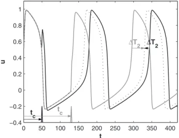
For the system we study in this paper, it turns out to be a good approximation to consider that the oscillator has reached its asymptotic new phase by the second action po-tential following the stimulation共i.e., we obtain virtually the same PRC and PTC if we wait for a third AP兲. Therefore, we measured ⌬in the following way共Fig.9兲.
Starting with initial conditions corresponding to the cho-sen phase zero 共u0⯝0.519, v0⯝−0.0149兲, we applied a stimulus at phase= tc/T0苸关0,1兲. For our Gaussian-shaped stimulus pulse, tcwas taken as the time at which the stimulus
goes through its maximum. The increment in phase from one trial to the next was at most 0.001共a smaller increment was used in the regions of phase where the PTC is particularly steep兲.
Following each stimulation, we waited for the occurrence of two APs and then measured the time tp2 at which the potential u 共solid traces in Fig. 9兲 goes through the “event
marker” 兵u=u0, du/dt⬎0其 on the second AP. Crossing this event marker is indeed equivalent to crossing phase zero when the state point is on the limit cycle. On the other hand, an unperturbed oscillator共dotted trace in Fig.9兲 would have
crossed the event marker on the same AP at t = 2T0. There-fore, the temporal shift between the two oscillators by the second AP is ⌬T2= 2T0− tp2 and the corresponding phase
shift共called the “second transient phase shift” 关73,75,76兴兲 is
⌬2=⌬T2/T0. As we stated above, no significant difference was observed when measuring instead ⌬T3 共temporal shift by the third AP兲, so that we could safely assume ⌬T⯝⌬T2 and ⌬⯝⌬2. On the other hand, there were significant differences between⌬T2 and⌬T1for some combinations of I0and.
The criterion we used to acknowledge the occurrence of an AP is that the potential u becomes greater than uAP = 0.706, which is the value of the potential at the right knee of the u-nullcline of the unforced system关see Fig.2共b兲兴. We
required additionally that the potential has first to decrease below 0 before a new AP can be elicited, so that deflections occurring during an AP共such as that caused by the stimulus in the black trace in Fig. 9兲 are not identified as additional
APs.
The phase shifts we measure are always smaller than 1, since the “best” a stimulus of short effective duration can do is to cause the immediate occurrence of one extra action potential. On the other hand,⌬can take all negative values; in particular it can be quite negative if the stimulus moves the state point close to the unstable fixed point of the system. Therefore we have⌬苸共−⬁,1兲.
Because a stimulus of sufficiently large amplitude is ca-pable not only of advancing or delaying an existing AP, but also of eliciting a new AP关see the first two animations
共tem-poral evolution of the potential兲 in supplementary material 关77兴兴, there can be discontinuities of size 1 in the PRC 共e.g.,
in Fig.10below兲 if ⌬is not defined modulo 1. Indeed, for large enough amplitude, there is a critical phase of stimula-tion such that, for a phase smaller than this value, the pertur-bation immediately caused by the stimulus in the u wave form does not satisfy the definition of an AP given above, while it does when the phase of stimulation is above the critical value 共this critical phase exists no matter the defini-tion of an AP chosen; only its value depends on the definidefini-tion used兲. At this threshold value of the phase, a discontinuity appears in the PRC. Its size is effectively 1 provided the state point is back to the limit cycle when the phase-shift measure-ment is done, which is virtually the case by the second AP here. Such size-1 gaps in the PRC do not make the PTC discontinuous since
⬘
is defined modulo one. Gaps of size different from 1 appear in the first transient phase shift⌬1, here共not shown兲 and elsewhere 关54,72–76兴, and lead todis-continuities in the PTC if ⌬1 is used to estimate ⌬. The reason we wish to keep track of the size-1 gaps in the PRC, by not using the modulo in the definition of ⌬, is given in the following section.
3. Phase-resetting map
In addition to its intrinsic interest as a characterization of the behavior of an oscillator, the PTC or PRC can be used to derive a one-dimensional 共1D兲 discrete map 共the “phase-resetting map”兲 which, under certain conditions, can predict the behavior of the oscillator under periodic forcing 共see, e.g.,关6,10,19,52–55兴兲. Suppose that the ith stimulus is given
when the state point of the system lies on the limit cycle, at phasei. Suppose also that it takes at most a timefor the
state point to come back, to within a good approximation共to be defined, but this definition does not matter to the present argument兲, to the limit cycle after having been perturbed away from it. Then, if the stimulation period T is larger than
, the state point will be effectively back to the limit cycle when the next stimulus is applied, at phase i+1. Calling
the phase at which the state point comes back to the limit cycle, we have
i+1=+
T − T0
共mod 1兲,
since the state point evolves on the limit cycle from to
i+1.is itself related toiby
=
⬘
共i兲 +
T0
共mod 1兲,
since
⬘
共i兲 is the asymptotic phase of the oscillatorstimu-lated at i when a hypothetically unperturbed oscillator
would crossi. So in the end we have
i+1= f共i兲 =
⬘
共i兲 +T
T0 共mod 1兲, 共5兲
where f is a one-dimensional circle map共discrete map from S1toS1兲 giving the phase just before the 共i+1兲st stimulus as a function of the phase just before the ith stimulus. It is obtained by simply shifting the PTC vertically by an amount
0 50 100 150 200 250 300 350 400 −0.4 −0.2 0 0.2 0.4 0.6 0.8 1 t u t c t c ∆T2 ∆T2
FIG. 9. Phase-shift measurement for two different trials with I0= 0.2共solid traces兲. The dotted trace shows the evolution of the u variable for the unperturbed oscillator. For tc= 50 共black trace兲,
⌬T2⬍0 共“phase delay”兲; for tc= 130共gray trace兲, ⌬T2⬎0 共“phase advance”兲.
T/T0, and its topological degree is therefore the same as that of the PTC. The fixed points of the Mth iterate of the map correspond to period-M solutions for the periodically forced oscillator. They will coincide with solutions of the original ODE 共1兲 when the hypothesis ⬍T is satisfied. One thus
expects the map to work better at large stimulation periods. Equivalent ways of formulating the justification for the use of 共5兲 can be found, e.g., in 关10,55,58兴.
An orbit of a circle map can be characterized by its rota-tion number. While this number was originally defined for degree-1 circle maps 共see Sec.II B兲, the definition has been
generalized to circle maps of any topological degree 关61兴.
共Note that this is different from generalizing the rotation number to 2D maps, as is done, e.g., in 关32兴.兲 Assume the
circle map f is defined by the restriction to the circle S of a map F :R→R, that is,
i= f共i−1兲 = F共i−1兲 共mod 1兲,
for i艌1. We use here F共x兲=x+⌬共x mod 1兲+T/T0. The ro-tation number for an initial condition0 is defined by
共f,0兲 = lim sup n→⬁ 1 n
兺
j=0 n ⌬j共j兲 共6兲 where⌬i−1共i−1兲 = F共i−1兲 −i−1.
For a periodic orbit of period M, 兵0*,*1, . . . ,M*其 with i* = f共 i−1 * 兲 and M *= 0
*, the rotation number is the rational number= N/M where
N =
兺
j=0 M−1
⌬j共j*兲.
The way we have defined⌬and F ensures that the criti-cal phases at which, in the PRCs, an extra action potential is generated, are preserved in F. This is important because it guarantees that the changes of rotation number that can occur along solution branches will be linked to our definition of an action potential, instead of being completely arbitrary. For instance, it guarantees that the stimulation period T/T0 at which, at large stimulation amplitudes, the 1:1 rhythm changes into the 1:2 rhythm along the period-1 branch共Fig.
11兲, will correspond to the generation of an extra action
po-tential according to our definition. If we had used instead F共x兲=
⬘
共x mod 1兲+T/T0, that stimulation period would have simply been T/T0= 1, which is meaningless. Use of the last-mentioned F共x兲, or adding the modulo in the definition of ⌬关Eq. 共3兲兴, is thus equivalent to erasing existinginfor-mation共the size-1 gaps in the PRC兲 and then artificially re-constructing it.
B. Results
1. Phase-resetting and phase transition curves
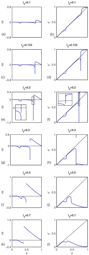
Figure 10 shows the evolution of the PRC and PTC for increasing stimulation amplitude, computed by the direct nu-merical integration method described in Sec. III A 2. For I0 −0.8 0 0.8 ∆φ I0=0.1 0 0.5 1 φ´ I0=0.1 −0.8 0 0.8 ∆φ I0=0.133 0 0.5 1 φ´ I0=0.133 −1.2 0 0.4 ∆φ I0=0.2 0 0 0.5 1 φ´ I0=0.2 −1 0 0.6 ∆φ I0=0.3 0 0.5 1 φ´ I0=0.3 −0.6 0 1 ∆φ I0=0.5 0 0.5 1 φ´ I0=0.5 0 0.5 1 −0.4 0 1.2 ∆φ I0=0.7 φ 0 0.5 1 0 0.5 1 φ´ φ I0=0.7 (c) (d) (e) (f) (g) (h) (i) (j) (k) (l) (a) (b)
FIG. 10. 共Color online兲 Evolution of the PRC 共left兲 and PTC 共right兲 for increasing stimulation amplitude I0. For I0= 0.1 and 0.133, the PRC is continuous and the PTC is of degree 1. For I0 = 0.2 and above, the PRC exhibits a discontinuity of size 1 and the PTC is of degree 0共zooms help to see this for I0= 0.2兲. The curves were computed using the direct numerical integration method de-scribed in Sec.III A 2.
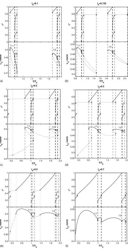
(a) (b) (c) (d) (e) (f) 1 1.2 1.4 1.6 1.8 2 0.47 0.48 0.49 0.5 T/T0 L2 −norm 1:1 1:2 0 0.2 0.4 0.6 0.8 1 φ* I0=0.1 0.8 1 1.2 1.4 1.6 1.8 2 2.2 2.4 0.4 0.42 0.44 0.46 0.48 0.5 0.52 T/T0 L2 −norm 1:1 1:2 0 0.2 0.4 0.6 0.8 1 φ* I0=0.133 0.2 0.6 1 1.4 1.8 2.2 0.2 0.3 0.4 0.5 T/T0 L2 −norm 1:1 1:2 0 0.2 0.4 0.6 0.8 1 φ* I0=0.2 0.2 0.6 1 1.4 1.8 2.2 0.25 0.3 0.35 0.4 0.45 0.5 T/T0 L2 −norm 1:1 1:2 0 0.2 0.4 0.6 0.8 1 φ* I0=0.3 0.2 0.6 1 1.4 1.8 2.2 0.3 0.35 0.4 0.45 0.5 T/T0 L2 −norm 1:1 1:2 0 0.2 0.4 0.6 0.8 1 φ* I0=0.5 0.2 0.6 1 1.4 1.8 2.2 0.4 0.45 0.5 0.55 T/T0 L2 −norm 1:1 1:2 0 0.2 0.4 0.6 0.8 1 φ* I0=0.7
FIG. 11. 共Color online兲 Com-parison of the period-1 solutions for the map and for the original ODE 共upper and lower sets of curves in each panel兲 for the val-ues of I0used in Fig.10. The lo-cations of the bifurlo-cations in the ODE are highlighted by vertical dashed 共SN兲 or dotted 共PD兲 lines. These lines look thick when two bifurcations occur for very close values of T/T0.
= 0.1 and 0.133, the PRC is continuous and the PTC has topological degree 1. For I0= 0.135, the steepness of the curves has become so large around ⬃0.78 that we could not determine their topology even by reducing the step in down to the minimum that double numerical precision al-lows共⯝15 significant decimal digits兲. That is why we do not show the PRC and PTC for this amplitude in Fig.10. To get round this difficulty, we used a method originally developed for the computation of 共un兲stable manifolds of vector fields 关78兴: we performed continuation of trajectories, defined as
the solutions of a boundary-value problem where the initial conditions are fixed to phase zero and the integration time is set to 3T0, using the phaseof the共single兲 stimulus given as the main continuation parameter. BecauseAUTOuses pseudo-arclength continuation 共which implies including the state variables in addition to the main parameter in the definition of the step兲, the continuation step size reflects the change of the entire computed trajectory, and not only the change of the main parameter 共as is the case of the step size in the direct numerical integration method used above兲. Therefore, we could follow much more finely, within the limits of double numerical precision, the evolution of the trajectories in the steeply changing region of the PTC. We could then deduce from the observed evolution that the topological degree is 0 at I0= 0.135. By repeating the procedure with different values of I0, we could show that the change of topological degree occurs for I0= Ith= 0.1338⫾0.0001, which is also the ampli-tude at which the merging of the period-1 loops with the everywhere-unstable period-1 branch takes place in the bi-furcation diagram of the original ODE. We explain the rea-sons for this coincidence in Sec. III B 4. In the supplemen-tary material关77兴, two animations made from the trajectories
computed by continuation provide a nice way to see that the PTC is degree 1 at I0= 0.133 and degree 0 at I0= 0.135: they show the evolution in the phase plane of the point corre-sponding to
⬘
共approximated by the point reached at t=tc+ 2T0兲 as the point corresponding towinds around the limit cycle once. They also reveal that the change of topological degree in the PTC of a relaxation oscillator involves canard-like trajectories: for in the steep region of the PTC, the trajectories hug the middle branch of the u-nullcline along a part of their course.
For all amplitudes above I0= 0.135 in Fig. 10, the PTC remains degree 0. Correspondingly, the PRC exhibits a dis-continuity of size 1, reflecting the fact that additional action potentials can be elicited for I0⬎Ith 共cf. the discussion in Sec. III A 2兲.
2. Qualitative features of the phase-resetting map Because the phase-resetting map is a simple vertical shift of the PTC, a few qualitative characteristics of the bifurca-tion diagrams for the 1D map can be deduced directly from the appearance of the PTCs in Fig.10. For I0= 0.1, the PTC is monotonic, so that no iterate of the 1D map can exhibit PD points. This is consistent with the bifurcation diagram of the original ODE 共Fig. 1兲, where none of the period-M loops
exhibits PD points. In addition, the PTC exhibits two down-ward deviations from the line of identity. This implies that there will be bistability between period-1 fixed points in the
map over a range of T/T0values共range over which the ver-tical shift of the PTC has four intersections with the line of identity兲. The corresponding range of 1:1 self-bistability is found in the bifurcation diagram of the ODE共Fig.1兲.
For I0= 0.133, the PTC is no longer monotonic, exhibiting regions with slope艋−1. This implies that even the first iter-ate of the 1D map共the “period-1 map”兲 will have PD points. This is consistent with the fact that even the period-1 loops exhibit PD points in Fig.5.
From I0= 0.2 to 0.7 in Fig.10, the PTC gradually flattens out, so that the ranges of T/T0over which the fixed points of the map are unstable gradually shorten. This agrees with the fact that the period-1 branch becomes stable over increas-ingly large ranges of T/T0 as I0 increases in the ODE共Fig.
8兲.
3. Period-1 map: Fixed points and their stability In order to compare quantitatively the predictions of the phase-resetting map with the results obtained for the original ODE, one needs to compute the fixed points of the map as a function of the stimulation period T/T0. In general, this re-quires solving a nonlinear algebraic equation for each value of the parameter, and continuation methods are often helpful in that process. However, for the kind of map we consider in this paper, where the parameter T/T0 appears in an additive fashion only, no computation is needed to determine the curves of fixed points for the period-1 map共first iterate兲, as we show below.
From 共4兲 and 共5兲, the period-1 map is
i+1=i+⌬共i兲 + T/T0 共mod 1兲, so that its fixed points *satisfy
⌬共*兲 + T/T0 共mod 1兲 = 0 or
*=共⌬兲−1关− T/T
0 共mod 1兲兴. 共7兲
Of course, for some values of T/T0, the inverse function 共⌬兲−1is not defined, or is multivalued, but共7兲 still provides a simple graphical way to obtain *as a function of T/T0. Indeed, 共7兲 implies that one simply needs to rotate the PRC
by 90° counterclockwise about the origin, and replicate the curve thus obtained at all distances equal to an integer along the T/T0 axis. Computations are needed only to locate the bifurcations along the curves of fixed points. The result of these operations for the six values of I0 from Fig. 10 are shown in the upper parts of the panels of Fig.11. The lower parts of the panels show the corresponding bifurcation dia-grams for the original ODE restricted to the period-1 solu-tions. Vertical dashed and dotted lines highlight, respectively, the locations of the SN and PD bifurcations for the ODE, in order to facilitate visual comparison with the bifurcations for the map 共which are only indicated by the usual crosses and circles兲.
Quantitative comparison confirms that the phase-resetting map does an excellent job in accounting for the period-1 bifurcations occurring in the ODE until rather small T/T0. For example, at I0= 0.5, the PD point occurring at T/T0
= 0.353777 in the ODE coincides with that found in the map up to the first six digits. The phase-resetting map does not however account for the everywhere-unstable period-1 branch existing at small stimulation amplitudes共Figs.1 and
5兲. This is because, for solutions belonging to this branch,
the state point never reaches the limit cycle of the unforced system共Fig.3兲, so that the phase of stimulation is not even
defined.
While the bifurcation diagrams in Fig. 11 allow a direct comparison between the two approaches insofar as the loca-tions of the bifurcaloca-tions are concerned, they do not allow comparison of all the solutions along the branches since the variables for the map and for the ODE are different. In order to make such a comparison, one would need to identify the phase of stimulation for the period-1 solutions of the ODE. The paradox is, however, that such an identification makes sense only when the map is a good approximation of the ODE, since phases are defined only for points belonging to the limit cycle of the unforced system. Nevertheless, one can always identify the point on the limit cycle closest to the state point at the moment when the stimulus is given, com-pute the phase corresponding to this point, and see how this phase compares with the phase predicted by the 1D map for the same stimulation period. Strictly speaking, this procedure does not yield a comparison between the two approaches共it is only a genuine comparison when the predictions of two approaches coincide, in which case it is pointless兲, but it does allow one to estimate the value of T/T0at which the 1D map approximation breaks down.
We have applied this procedure to a sample of the peri-odic solutions from the left part of the period-1 branch for I0= 0.2 关T/T0⬍1.1 in Fig. 8共a兲兴. The moment at which the
stimulus starts is assumed to be tm3= tst− 3, where tstis the time at which the Gaussian-shaped stimulus goes through its maximum, since the effect of the stimulus can still be con-sidered to be negligible before t = tm3. The coordinates of the
state point at that moment are then compared to those of a stored array of points on the limit cycle共obtained via a pre-liminary integration兲 to determine which of these points is the closest to the state point. We use a weighted Euclidean distance as our metric, with a ten times larger weight for the v variable since it varies over a range about ten times smaller than the u variable. The phasem3of the closest point on the
limit cycle is then identified共this is straightforward provided the preliminary integration is started at phase zero, and that time is stored at each step in addition to the coordinates of the points兲. We then compare the phase ˆ =m3+ 3/T0 共mod 1兲 to the phase * predicted by the map, since the latter is defined considering the time at which the Gaussian-shaped stimulus goes through its maximum. This method has been used previously as an alternative to the method de-scribed in Sec.III A 2to determine the PTC关7兴.
Figure 12共a兲shows the projections onto the 共u,v兲 phase plane of the period-1 solutions for the ODE, labeled by a number that increases as T/T0decreases共the solutions num-bered 21, 23, and 25 are not shown for the sake of clarity兲. The circle symbol on each trajectory represents the coordi-nates of the state point at t = tm3and the corresponding cross
represents the closest point on the limit cycle 关the crosses 共circles兲 corresponding to the solutions numbered 7–22
ap-pear superimposed in Fig.12共a兲because they correspond to very close stimulus phases; see Fig. 12共b兲兴. Figure 12共b兲 shows the phases computed for the solutions in Fig. 12共a兲 共numbered colored dots兲, superimposed on the phases pre-dicted by the map共solid black curve兲. The two sets of phases start to diverge around T/T0= 0.3. The discrepancy involves, as expected, the solutions with number 24 and above, since these are the solutions in Fig.12共a兲for which the circles and crosses do not coincide, i.e., solutions for which the assign-ment of a phase does not make sense. Also nicely illustrated in Fig. 12共a兲is the canardlike behavior of most of the un-stable limit cycles along this branch共only the periodic tions labeled 1 to 4, which are stable, and the periodic solu-tion labeled 26, which is unstable, do not hug the middle branch of the u-nullcline along a part of their course兲.
0.1 0.3 0.5 0.7 0.9 1.1 0.2 0.3 0.4 0.5 0.6 0.7 0.8 0.9 T/T0 φ* 1 2 3 46 7 8 9 10 11 13 14 15 16 17 18 19 20 21 22 23 24 25 26 −0.2 0 0.2 0.4 0.6 0.8 1 −0.02 0 0.02 0.04 0.06 0.08 0.1 0.12 0.14 u v 12 3 45 6 7 8 9 10 11 12 13 14 15 16 17 18 19 20 2224 26
(a)
(b)
FIG. 12.共Color online兲 共a兲 projections onto the phase plane of a sample of period-1 solutions of the ODE for I0= 0.2共0.05⬍T/T0 ⬍1.1兲. The unlabeled solid black curve is the limit cycle of the unforced system, the dashed curves are the nullclines, and the num-bered colored curves are the periodic solutions of the ODE. See text for details. 共b兲 phases computed for the solutions shown in 共a兲 共numbered colored dots兲 and phase predicted by the corresponding period-1 map共solid black curve兲.
4. Period-1 map: Topology of solution branches It is not a coincidence that the topological degree of the PTC changes at the same amplitude Ithas that at which the period-1 loops merge with the everywhere-unstable period-1 branch in the bifurcation diagram of the original ODE. In-deed, Eq. 共7兲 implies that the fixed points of the period-1
map belong to isolated loops when the PTC is of degree 1 and to a unique branch when the PTC is of degree 0, as we explain now. Since⌬=
⬘
−, the mean slope of the PRC is obtained by subtracting one from the mean slope of the PTC. Thus, when the PTC is of degree 1, the PRC has a mean slope equal to 0. Rotating the PRC by 90° counterclockwise, to obtain the period-1 fixed points, gives a curve with infinite mean slope, that is, a deformation of a vertical line. The ends of this curve, = 0 and = 1, thus have the same abscissa T/T0. Because= 0 is the same phase as = 1, the curve is actually a closed loop. The bifurcation diagram for the period-1 map is thus made up of the replication of the same loop every unit along the T/T0 axis 关e.g., upper curves in Figs.11共a兲and11共b兲兴. In contrast, when the map is of degree 0, the PRC has a mean slope equal to −1, which implies that the curve of period-1 fixed points has a mean slope equal to 1. Its ends = 0 and = 1 thus span a distance of 1 on the T/T0axis, so that the replication of the curve every unit of T/T0 gives in this case a unique continuous branch 关e.g., upper curves in Figs. 11共c兲–11共f兲兴. Hence, the bifurcationdiagram of any circle map of the form 共5兲 has its period-1
fixed points belonging to isolated loops when the topological degree of the map is one, while they belong to a unique branch when the degree is zero. To our knowledge, this to-pological property of circle maps had not been underscored before.
As a consequence, if the 1D map is a good approximation of the original ODE, one would expect a change in degree in the map at the same stimulation amplitude as that at which the period-1 loops in the bifurcation diagram of the original ODE merge with the everywhere-unstable period-1 branch, which indeed is what happens. However, it is important to remember that the 1D map does not account for the everywhere-unstable period-1 branch that exists at small stimulation amplitudes in the original ODE, and whose pres-ence is crucial to the merging phenomenon: from a topologi-cal point of view, the period-1 loops could not form an un-bounded period-1 branch for I0⬎Ith if they were not to collide with an unbounded period-1 branch.
The important role of the everywhere-unstable period-1 branch in the main topological change of the bifurcation dia-gram of the ODE is not surprising to the extent that it reflects the existence of the unstable fixed point of the unforced sys-tem. Indeed, for planar oscillators described by a stable limit cycle surrounding a single unstable fixed point, the fixed point is known to be crucially implicated in the change of topological degree of the PTC. In the case of a stimulus of finite duration, the change of topological degree occurs when the “shifted cycle,” the locus of the state reached at the end of the stimulus by all the points belonging initially to the limit cycle, intersects the unstable fixed point关79兴. However,
the notion of a shifted cycle is not really defined for a stimu-lus with no clear end such as the one we use in this paper.
5. Period-M maps and translational symmetry of the bifurcation diagram
The translational symmetry that characterizes the bifurca-tion diagram for the fixed points of the period-1 map actually extends to the fixed points of all iterates 共period-M maps兲, due to the additive dependence of the map on the bifurcation parameter T/T0 关Eq. 共5兲兴. Physically, this corresponds to the fact that stimulating the oscillator at time t or at time t + T0 does not make any difference when the state point lies on the limit cycle, since the phase of stimulation will be the same. More precisely, given a circle map of the form 共5兲, if
兵1*, . . . ,
M
*其 is a period-M orbit for T=T* with rotation number= N/M, then 兵1*, . . . ,M*其 is also a period-M orbit for T = T*+ KT0, where K is any positive integer, and its ro-tation number is=共N+KM兲/M 关19,61兴.
As a consequence, and because we know that the phase-resetting map accounts almost perfectly for the solutions of the ODE at large stimulation periods, one way to evaluate how the map succeeds in approximating the original ODE at small stimulation periods is to determine to what extent the translational invariance is present in the bifurcation diagrams for the ODE. This indirect method is the only procedure we will use to compare the period-M orbits of the map to the period-M solutions of the ODE for M⬎1, i.e., we will not explicitly compute fixed points of the period-M maps.
The translational invariance predicted by the map is well verified in the bifurcation diagram of the ODE for I0= 0.1 共Fig.4兲, since even the bifurcations on the 3:1 loop coincide
visually with those of the 3:4 loop, when the later are shifted by −1共the left SN is at T/T0= 0.307 797 for the 3:1 loop and at T/T0= 0.307 795 for the 3:4 loop, while the locations of the right SNs coincide up to 6 digits兲. For I0= 0.133 共Fig.
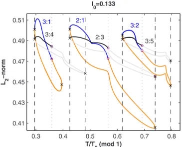
13兲, however, a large discrepancy is present at the right of
the 3 : 1/3:4 loops, whereas the left SNs still coincide up to six decimal digits. This might seem surprising, since one expects a priori the 1D map approximation to break down at the smallest stimulation periods, where the state point gets the smallest amount of time to recover back to the limit cycle following a perturbation. However, at the right end of the 3:1 loop, the stimulus falls at just the right phase to kick the state point near to the fixed point of the unforced system, where the dynamics is very slow. Thus, even if there is more time to recover than at smaller stimulation periods, there is still not enough time to allow the state-point to return to the limit cycle before the next stimulus occurs – hence the 1D map approximation breaks down.
The picture for I0= 0.135 is even more striking 关Figs.
14共a兲and14共b兲兴, with the 3:4 loop being completely differ-ent from the 3:1 loop关Fig.14共a兲兴, and the 2:3 having become
a branch while the 2:1 is still a loop 关Fig.14共b兲兴. The phe-nomenon does not occur for I0= 0.1 共Fig. 4兲 because the stimulation amplitude is not large enough to kick the state point from the limit cycle to near the fixed point, and it does not happen for I0= 0.5 关Figs. 14共e兲 and 14共f兲兴 because the
stimulation amplitude is too large to do so. For I0= 0.2关Figs.
14共c兲 and14共d兲兴, a small discrepancy is still present at the right end of the period-3 loops, but it is much smaller than the discrepancy at the left end.
IV. DISCUSSION
A. Continuation applied to pulse-forced oscillators in relaxation regime
In electrophysiology, one is often interested in relaxation oscillators forced with a periodic train of pulsatile stimuli, the duration of each stimulus being considerably shorter than the intrinsic period. However, the vast bulk of the work on forced oscillators has been for sinusoidally forced systems, and such forcing can lead to behaviors that are qualitatively different from those seen with pulsatile forcing: e.g., with sinusoidal forcing one can have bursting rhythms that one does not see with pulsatile forcing, in which several action potentials ride on the crest of each cycle of the sinusoidal input共see, e.g., Fig. 16 of 关39兴兲. In addition, many of these
studies on sinusoidal forcing have been in the nonrelaxation regime of the oscillator.
One major advantage of continuation methods is that un-stable orbits, as well as un-stable ones, can be tracked. While there have been a few studies using continuation techniques to investigate pulsatile forcing in the nonrelaxation regime 关29,32,37兴 and one study on sinusoidal forcing in the
relax-ation regime 关13兴, we are not aware of any continuation
analyses on pulsatile forcing in the relaxation regime. In trast with the aforementioned studies, we have applied con-tinuation to the ODE itself, not to a stroboscopic map of it, in order to benefit from existing functionalities of the AUTO
continuation software. However, while it is rather straightfor-ward to run AUTO on sinusoidally forced systems 共see the demo “frc” in the AUTO manual 关62兴兲, this is not true for
most other functional forms of forcing. We have used a re-cently described method that allows one to useAUTOto study
an ODE in which the forcing term is not expressed in terms
of sines and cosines, necessitating only minor modifications of theAUTOsource code关48兴. This method is similar in spirit
to one used previously to study stroboscopic maps of forced oscillators共e.g., 关23兴兲, in that it takes advantage of the fact
that the period of any periodic orbit has to be an integer multiple of the forcing period.
Had we not been led by the results obtained via continu-ation methods in the ODE, we would probably not have no-ticed the topological property of the bifurcation diagrams of circle maps which constitutes one of the main findings of this paper.
B. The topology of phase resetting
As I0 is increased, we find a transition from a degree-1 invertible PTC to a degree-1 noninvertible PTC to a degree-0 PTC 共Fig.10; see also 关9,55兴兲. All these three types of PTC
have been reported previously in the FHN oscillator 关6–8,10兴.
A simple continuity argument shows that at a sufficiently low stimulation amplitude, the PTC has to be of degree one and invertible, while at a sufficiently high stimulation ampli-tude, it has to be of degree zero 关59兴. A degree-1 curve can
be invertible or not, while a degree-0 curve is, by definition, noninvertible. In models that are intrinsically discontinuous, as stimulation amplitude is increased, there can be a direct transition from a degree-1 invertible PTC to a degree-0 PTC 共e.g., 关19,26,34,80,81兴兲. In continuous models, there is often
a transition from a degree-1 invertible curve to a degree-1 non-invertible curve, and then to a degree-0 curve 关9,14,58,73兴. There are also several other studies
demonstrat-ing parts of this sequence: e.g., the transition from invertibil-ity to noninvertibilinvertibil-ity of a degree-1 PTC 关54兴 or from a
degree-1 noninvertible to a degree-0 PTC 关26,30兴. There
have been very few systematic studies on noninvertible degree-1 PTCs. In one experimental study, the PTC was found to be noninvertible over about 50% of the range of amplitude over which it was of degree 1 关54兴, which is a
larger range than we find above共at most 25%兲.
Even at the lowest I0, there are three bumps in the PRC of our oscillator. For example, at I0= 0.1 关Fig.10共a兲兴, the first bump 共at = 0.2– 0.3兲 is caused by the stimulus extending the duration of the action potential 关as can be seen, e.g., in the black trace in Fig. 2共a兲兴. The second bump, at = 0.7– 0.8 for I0= 0.1关Fig.10共a兲兴, is due to a prolongation of
the “diastolic interval,” which is the time between the end of the action potential and the start of the subsequent action potential 关gray trace in Fig. 2共a兲兴. The third bump is at = 0.8– 1.0 and is caused by a shortening of the diastolic in-terval by the stimulus 共the gray trace in Fig.9 shows this effect for I0= 0.2兲. While there are cases in experimental 共e.g., 关54,72兴兲 and modeling 关73–75兴 work on cardiac
oscil-lators where one can see all three of these bumps in the same PRC, the amplitude of the first bump is usually considerably less pronounced than in the FHN oscillator. As we discuss below, the amplitude of this bump has an important conse-quence in determining whether or not 1:1 self-bistability will be observable.
C. Discontinuities in the PTC
We have mentioned above共Sec.III A 2兲 that an artifactual
discontinuity can arise in the PTC if the oscillator is not
0.3 0.4 0.5 0.6 0.7 0.8 0.41 0.43 0.45 0.47 0.49 0.51 T/T0(mod 1) L 2 −norm I0=0.133 3:1 3:4 2:1 2:3 3:2 3:5
FIG. 13.共Color online兲 Evaluation of the translational symmetry in the bifurcation diagram of the original ODE for I0= 0.133, using the procedure and conventions described in Fig.4. Here, in addi-tion, vertical dotted lines highlight the locations of the PD points for the shifted loops. The period-1 loops are not shown since their symmetry under translation can be deduced from the comparison with the fixed points of the period-1 map共Fig.11兲.