1 ATTEL PROJECT
PERFORMANCE-BASED APPROACHES FOR HIGH STRENGTH TUBULAR COLUMNS AND CONNECTIONS UNDER EARTHQUAKE AND FIRE LOADINGS
Deliverable 5 – Model calibration
D.5.1. : Definition of stability curves
D.5.2. : D5.2: simulation data relevant to the selected typologies of base-joints, of HSS-CHS columns and HSS-CFT columns and of HSS-concrete composite beam-to-column joints
D.5.3. : Report on parametric numerical analyses
Contributing Partners: Stahlbau Pichler University of Liège Centro Sviluppo Materiali University of Thessaly University of Trento
2
Summary
D.5.1. Definition of stability curves ... 3
D.5.1.A. Recommended practice for Planning, Designing and Constructing Fixed Offshore Platforms- Load and Resistance Factor design [3] ... 3
A.1. Axial Compression ... 3
A.2. Bending ... 4
A.3 Combined Axial Compression and Bending ... 4
D.5.1.B. Eurocode3: Design of steel structures ... 5
B.1. Buckling strength in axial compression for tubular sections ... 5
B.2. Bending ... 9
B.3 Combined loads ... 10
D.5.1.C. Structural stability of hollow sections [6] ... 11
C.1 Tubular Members in axial compression for class 1, 2 & 3 ... 11
C.2 Tubular members in bending for class 1, 2 &3 ... 11
C.3 Members in combined compression and bending class 1, 2 & 3 ... 11
D.5.1.D. AISC-Load and Resistance Factor Design Specification for HSS Sections ... 12
D.1. Design Requirements ... 12
D.2 Tubular Compression Members ... 12
D.3. Beams and other Flexural Members ... 13
D.4 Members under Combined Forces ... 13
D.5.2. Simulation data ... 14
D.5.2.1. Simulation Data of HSS Columns ... 14
D.5.2.1.1. Model description ... 14
D.5.2.1.2. Finite element model Main Results ... 15
D.5.2.1.3. Conclusions ... 18
D.5.2.2. Numerical analysis for columns in fire condition ... 18
D.5.2.3. Simulation data of column-base and beam-to-column joints ... 22
D.5.2.2.1. Hysteretic behaviour of both beam-to-column and column-base joints ... 22
D.5.2.2.2. Mechanical behaviour of a plinth relevant to an innovative seismic joint ... 28
D.5.2.4. Numerical analysis of connections in fire condition………..29
D.5.2.5. Numerical analysis for vertical plate of static joints………...44
D.5.2.6. Numerical analysis for “end plate” component of static column bases………...49
D.5.3. Parametric numerical analysis………...53
D.5.3.1. Analysis of the behaviour of columns at room temperature ... 53
D.5.3.1.1. Buckling response of axial loaded tubular members ... 54
D.5.3.1.2. Analysis of the prototype structure under seismic loading………56
D.5.3.2. Parametric study for the vertical plate of static joints………..59
D.5.3.3. Parametric study for the end plate of static column bases………...………..…..59
Appendix A………...60
References……….61
3
D.5.1.
Definition of stability curves
In this section, the stability curves and axial load - bending interaction diagrams for tubular beam-columns as proposed in four major design specifications are presented in detail. The specifications are the API RP2A LRFD, Eurocode 3 (EN 1993), the CIDECT guidelines No.3, and the AISC specifications for Hollow Structural Sections, Those specifications are evaluated using experimental and numerical results from the present research in subsequent sections.
D.5.1.A.
Recommended practice for Planning, Designing and Constructing
Fixed Offshore Platforms- Load and Resistance Factor design [3]
A.1. Axial Compression
The recommendations given in this section are applicable to stiffened and unstiffened cylinders having a thickness t≥6mm, diameter-to-thickness ratio D /t < 300 and having yield strengths less than 414 MPa (60 ksi).
1.1.1.1. A.1.1. Column Buckling
The nominal axial compressive strength for tubular members subjected to column buckling should be determined from the yield stress according to the following equations:
2 cn y
F = 1.0-0.25λ
F
for λ < 2 (A.1.1-a) cn 2 y 1 F = F λ for λ ≥ 2 (A.1.1-b) whereλ= column slenderness parameter defined as follows:
0.5 y F ΚL λ= πr Ε (A.1.1-c) where
Fcn= nominal axial compressive strength, in stress units
E= Young’s modulus o elasticity K= effective length factor L=embraced length r= radius of gyration A.1.2 Local Buckling
The possibility of local buckling of the tubular members should be examined calculating the elastic and inelastic local buckling stresses as follows:
a) Elastic Local Buckling
The nominal elastic local buckling strength should be determined from:
( )
xe x
F =2C E t/D
(A.1.2-1)where
xe
F =nominal elastic local buckling strength, in stress value
x
C = critical elastic buckling coefficient D= outside diameter
t= wall thickness
4 The theoretical value of Cxis 0.6. However, a reduced value of Cx=0.3 is recommended for use in the above equation to account the effect of initial imperfections.
b) Inelastic Buckling
The nominal inelastic local buckling strength should be determined from:
xc y
F =F
for D 60 t ≤ (A.1.2-2)( )
1/4 x c yF = 1.64-0.23 D/t
F
for D 60 t > (A.1.2-3) Where x cF = nominal inelastic local buckling strength, in stress units
In case that Fxc < Fy, or Fxe <Fy a cylindrical member in compression is possible to fail due to local
buckling. In order to calculate global (column) buckling, the nominal yield strength (Fy) in Eqs
(A.1.1-a) & (A.1.1-b) is replaced by the minimum value between the nominal inelastic local buckling strength (Fxc) and the nominal elastic local buckling strength (Fxe).
A.2. Bending
The nominal bending strength (in stress units) for tubular members should be determined from the following equations in terms of the yield stress Fy and the diameter-to-thickness ratio:
pl bn y el W F = F W (A.2-a) For D/t ≤ 10340/Fy (Fy in MPa) For D/t ≤ 1500/Fy (Fy in ksi) y pl bn y el F D W F = 1.13-2.58 F Et W (A.2-b) For 10340/Fy ≤D/t ≤ 20680/Fy (Fy in MPa) For 1500/Fy <D/t ≤3000/Fy (Fy in ksi) y pl bn y el F D W F = 0.94-0.76 F Et W (A.2-c) For 20680/Fy ≤D/t ≤ 300 (Fy in MPa) For 3000/Fy <D/t ≤ 300 (Fy in ksi) Where
Fbn nominal bending strength, in stress units
Wel elastic section modulus
2 el m
W =πR t
Wpl plastic section modulus
2 pl m
W =4R
t
A.3 Combined Axial Compression and Bending
Cylindrical members under combined axial compressive and bending loads should be designed to satisfy the mimimum of the following conditions:
5 by c c cn bn ey f f 1 + 1.0 f F F 1-F ≤ (A.3-a) and by c xc bn f f π 1-cos + 1.0 2 F F ≤ (A.3-b) where
fc , compressive stress due to factor loads (fc<φc Fcn)
fb, bending stress due to factor loads(fb<φb Fbn)
Fcn, nominal axial compressive strength calculated in Eqs A.1, in stress units
Fbn nominal bending strength calculated in Eqs A.2, in stress units
φc=1, the resistance factor for axial compressive strength
φb=1, the resistance factor for bending strength my
C
reduction factor corresponding to the member y axis defined equal to 1 from the table D.3-1ey
F
Euler buckling strength corresponding to the member y axis, in stress unitsy ey 2 y
F
F =
λ
(A.3-c)λy column slenderness parameter defined by Equation (B.1.1.1-c) [(D.2.2-2c)], where the parameters K,
L and r are chosen to correspond to the bending about the y direction.
D.5.1.B.
Eurocode 3: Design of steel structures
In order to calculate the buckling stress of a tubular member, the classification of the tubular cross section should be determined in accordance to Table 1.
Table 1 Classification limits for tubular cross-sections
B.1. Buckling strength in axial compression for tubular sections
When the tubular cross section is identified as class 1, 2 &3 then following procedure is followed according to EN-1993(part 1-1), otherwise, when class 4 is considered EN-1993-1-6 [EN-1993-1-6, 2007]should be followed:
6 The buckling strength under axial compression for a tubular member is defined as follows
b,Rd y
N
=χAf
for class 1, 2 and 3 (B.1.1-1)where
b,Rd
N
: buckling strength under axial compressionχ: reduction factor for the corresponding buckling mode A : area of the tubular cross section
For members subjected to axial compression,χvalue is defined in terms of member slenderness as follows: 2 2 1 χ = Φ+ Φ -λ (B.1.1-2) where:
(
)
2Φ=0.5 1+α λ-0.2 +λ
(B.1.1-3) and y cr cr 1 Αf L 1 λ= =Ν i λ for class 1, 2 and 3 (B.1.1-4)
where
Lcr: the effective buckling length
i : radius of gyration 1 y E λ =π =93.9ε f (B.1.1-5) y 235 ε = f (fy in N/mm 2 ) (B.1.1-6)
α : imperfection factor is defined in Table 2 ( Section 6.1) based on the buckling curve Table 6.2(see EN-1993-1-1)
Table 2. Imperfection factors for stability curves
Buckling curve a0 a b c D
α 0.13 0.21 0.34 0.49 0.76
The buckling curve for hot-formed steel tubular members should be obtained from Table 6.2 (see EN-1993-1-1). For S235/ 275/ 355/ 420, “a” buckling curve is obtained and for S460 the “a0”.
When the tubular cross section is identified as class 4, the procedure below is followed according to EN-1993(part 1-6)[EN -1993-1-1, 2007]:
B.1.2 Buckling Strength Class4
In order to define the buckling curves for class 4 sections, we follow the procedure described below: For class 4 cross sections the global relative member slenderness should be obtained from:
x,Rd Rcr N λ=
Ν (B.1.2-1)
Nx,Rd accounts for the critical meridional buckling load and NRcr accounts for the Eulerian elastic critical
7
x,Rd x,Rd
N
=σ
Α
(B.1.2-2)The elastic meridional stress (
σ
x,Rd) is defined according to the provisions of Annex D of EN-1993-1-6 as described in the following Sections (Section B.1.2.1) and the cross section area is denoted as A.( )
2 Rcr 2ΕΙ
Ν
= π
kL
(B.1.2-3)where E is the elastic Young modulus, I is the inertia of the cross section and k is the effective buckling length factor based on the boundary conditions
In this case the buckling load (NRd) is defined as follows: Rd x,Rd
N =χ(λ)σ
Α
(B.1.2-4)where the factor χ(λ) is obtained from the combination of Eqs B.1.1-2, B1.1-3 and B.1.2-1 a. B.1.2.1 Local buckling stress design
(1)The buckling resistance should be represented by the buckling stresses as defined in 1.3.6. The design buckling stresses should be obtained from:
x,Rd x,Rk Μ1
σ
=σ
/γ
(B.1.2.1-1)(2)The characteristic buckling stresses should be obtained by multiplying the characteristic yield strength by the buckling reduction factor χ:
x,Rk x yk
σ
=χ f
(B.1.2.1-2)(3)The buckling reduction factor χx should be determined as a function of the relative slenderness of the
shell λ from: χ=1 when λx≤ λ0 (B.1.2.1-3a) η x 0 p 0
λ -λ
χ = 1- β
λ -λ
when λ0< λx< λp (B.1.2.1-3b) 2 x α χ = λ when λp ≤ λx (B.1.2.1-3c) whereα : elastic imperfection reduction factor β : plastic range factor
η : interaction component
λ0 : squash limit relative slenderness
The values of the above parameters (α, β, η, λ0) should be taken from Annex D described below in
section B.1.2.2
The value of the plastic limit relative slenderness λp should be obtained from: p
α
λ =
1-β
(B.1.2.1-4)The relative shell slenderness parameter should be determined from:
yk x x,Rcr f λ = σ (B.1.2.1-5) b. B.1.2.2 - ANNEX D
8 B.1.2.2.1 Elastic critical meridional buckling stress
(1)The following expressions may only be used for shells with boundary conditions BC1 or BC2 defined in Table 5.1 section 5 of EN-1993-1-6.
(2)The length of the shell segment is characterized in terms of the dimensionless length parameter ω:
l r ω =
r t (B.1.2.2-1)
where
l: cylinder length between defined boundaries r: radius of cylinder middle surface
t: thickness of shell
(3) The elastic critical meridional buckling stress (
σ
x,Rcr), should be obtained from:x,Rcr x
t σ =0.605ΕC
r (B.1.2.2-2)
where Cx depends on the value of ω (see EN-1993-1-6, ANNEX D).
(3a) For medium-length cylinders, which are defined by:
1.7≤ ω ≤ 0.5 r/t (B.1.2.2-3)
The factor Cx should be taken as:
Cx=1.0 (B.1.2.2-4)
(3b) For short cylinders, which are defined by:
ω ≤ 1.7 (B.1.2.2-5)
The factor Cx should be taken as:
x 2
1.83 2.07 C =1.36- +
ω ω (B.1.2.2-6)
(3c) For long cylinders, which are defined by:
ω > 0.5 r/t (B.1.2.2-7)
The factor Cx should be taken as: x x,N
C =C
(B.1.2.2-8)In which Cx,N is the greater of:
x,N xb 0.2 t C =1+ 1-2ω C r (B.1.2.2-9) And x,N
C
=0.60
(B.1.2.2-10)where Cxb is a parameter depending on the boundary conditions and being taken from table D.1
(3d) For long cylinders as defined in (3c) that satisfy the additional condition:
r 150 t≤ and r ω 6 t ≤ and y,k E 500 1000 f ≤ ≤ (B.1.2.2-11)
9 xE,N xE,M x x,N xE xE σ σ C =C + σ σ (B.1.2.2-12) where
σxE is the design value of meridional stress σxE,d
σxE,N is the component of σxE,d that derives from axial compression (circumferentially uniform
component)
σxE,M is the component of σxE,d that derives from tubular global bending (peak value of the
circumferential varying component)
The following simpler expression may also be used in place of expression (B.1.2.2-12)
xE,M x xE σ C =0.6+0.4 σ (B.1.2.2-13)
B.1.2.2.2 Meridional buckling parameters
(1) The meridional elastic imperfection reduction factor αx should be obtained from:
(
)
1.44k
0.62
α =
1+1.91 ∆w /t
(B.1.2.2-14)where ∆wk is the characteristic imperfection amplitude:
k
1
r
∆w =
t
Q
t
(B.1.2.2-15)(2) where Q is the meridional compression fabrication quality parameter which should be taken from the table D.2 (See EN-1993-1-6) for the specified fabrication tolerance quality class
(3)The meridional squash limit slenderness λ0, the plastic range factor β, and the interaction exponent η
should be taken as:
λ0=0.20 β=0.60 η=1.0
(B.1.2.2-16)
(4) For long cylinders that satisfy the special conditions of B.1.2.2.11, the meridional squash limit slenderness λ0 may be obtained from:
xE,M 0 xE σ λ =0.20+0.10 σ (B.1.2.2-17) where
σxE is the design value of the meridional stress σxE,d
σxE,M is the component of σxE,d that comes from tubular global bending (peak value of the
circumferential varying component)
(5) Cylinders need not be checked against meridional shell buckling if they satisfy:
yk
r E
0.03
t ≤ f (B.1.2.2-18)
B.2. Bending
The classification of the cross section should be defined from Table 5.2 of Eurocode 3 (EN-1993-1-1): Design of steel structures.
B.2.1 Bending Class 1, 2 & 3 [EN-1993-1-1, 2005]
10 Ed c,Rd M 1.0 M ≤ (B.2.1-1)
(2)The design value of bending moment is defined as follows:
c,Rd pl,Rd pl y
M
=M
=W f
class 1 or 2 (B.2.1-2a)c,Rd el,Rd el,min y
M
=M
=W
f
class 3 (B.2.1-2b)where
Wpl is the plastic section modulus
Wel is the elastic section modulus
B.2.2 Bending Class 4 [EN-1993-1-6, 2007] The design bending strength is defined as follows:
x,Rd el x,Rd
M
=W σ
(B.2.2-1)where
x,Rd
σ
should be obtained from the equation (B.1.2.1-1) of EN1993-1-6 [7] and Cx may be obtained byequation (B.1.2-12) or (B.1.2-13), considering xE,M
xE σ =1.0 σ and xE,N xE σ = 0
σ , for pure bending.
B.3 Combined loads
B.3.1 Class 1, 2 & 3 [EN-1993-1-1, 2005]
Classification of cross section is estimated in Table 5.1 (see EN-1993-1-1)
The stability of members with constant cross section not susceptible to torsional displacements (i.e. tubular members) should satisfy the following equations:
Ed Ed yy Rd Rd N M +k 1.0 χN M ≤ (B.3.1-1) Where
NEd, My,Ed are the design values of the axial compression and bending strength
χ reduction factor due to flexural buckling
kyy interaction factor obtained from Annex A(Method1, see EN-1993-1-1)
For the interaction equation [B.3.1-1] simply supported members are considered with or without lateral supports subjected to axial compression and bending moments or lateral loads.
B.3.2 Class 4 [EN-1993-1-6, 2007]
The methodology proposed is described and the interaction curve is defined similar to section B.3.1, Eq (3.1-1): Ed Ed yy Rd x,Rd N M +k 1.0 N M ≤ (B.2.3.2-1) where
NRd is the axial load calculated in Eq. B.1.2-4 considering pure compression for class 4 cross sections
according to EN-1993-1-6
Mx,Rd is the moment strength calculated in Eq B.2.2-1 considering pure bending for class 4 cross
sections according to EN-1993-1-6
11
D.5.1.C.
Structural stability of hollow sections [6]
The classification of the tubular cross sections is defined from Table 4 (page 14) similar to EN1993-1-1 [9].
C.1 Tubular Members in axial compression for class 1, 2 & 3
The design buckling load of a compression member is given by the condition:
d b,Rd
N
≤
N
(C.1-1)Where
Nd is the working load and Nb,Rd is the design buckling resistance capacity of the member b,Rd y
N
=χAf
for class 1, 2 and 3 (C.1-2)where χ accounts for the reduction factor of the relative buckling curve (Figure 3, Tables 11 -14) depending on the non-dimensional slenderness value (λ) of a column.
The buckling curves can be defined analytically by the equations (B.1.1-1&2) as described in EN-1993-1-1. Similarly, the member slenderness is calculated by Eq (B.1.1-4). The buckling curve for hot-formed high strength steel should be obtained from Table 10b (see [6]) or Table 6.2 (see EN1993-1-1 [9]).
It is noted that for grades S235/ 275/ 355/ 420, buckling curve “a” should be considered, while “a0”
curve corresponds to grades greater than S460.
C.2 Tubular members in bending for class 1, 2 &3
The design value of bending moment is defined similar to EN-1993-1-1 provisions described in B.2.1: C.3 Members in combined compression and bending class 1, 2 & 3
The relation of compression and bending strength is based on the following linear interaction formulae:
Sd Sd y b,Rd Rd N M +K 1 N M ≤ (C.3-1) Where
Nsd is the design value of axial compression
Nb,Rd is the buckling load and is defined as follows: b,Rd pl y
N
=χN =χΑf
(C.3-2)χ is the buckling reduction factor defined in section B.1, and fy accounts for the yield strength
Msd is the maximum absolute design value of the bending moment about y-y axis according to the first
order theory.
MRd is the bending cross sectional strength defined as described previously in Section B.2.1 Sd y y pl N K =1- µ χN , however Ky ≤ 1.5 (C.3-3)
(
)
pl y y M,y el W µ =λ 2β -4 + -1 W , however µy<0.9 (C.3-4) whereβΜ,y is the equivalent uniform moment factors according to Table 16, column2(see [6]), in order to
12
D.5.1.D.
AISC-Load and Resistance Factor Design Specification for Steel Hollow
Structural Sections [2]
D.1. Design Requirements D.1.1. Classification of Steel Sections
HSS are classified for local buckling of the wall in compression as compact, noncompact,or slender-element cross-sections according to the limiting wall slenderness ratios λp and λr in Table 2.2-1 (see
[2]). For an HSS to qualify as compact, the wall slenderness ratio λ must be less than or equal to λp. If λ
exceeds λp but is less than or equal to λr, the HSS is noncompact. If λ exceeds λr, the HSS is a
slender-element cross-section. The wall slenderness ratio λ shall be calculated as follows:
(a) For round HSS, λ = D/t, where D is the outside diameter and t is the wall thickness. This Specification is applicable only to round HSS with λ less than or equal to 0.448E/Fy, where
E is the modulus of elasticity and Fy is the specified minimum yield stress.
D.1.2 Design by Plastic Analysis
Design by plastic analysis is permitted when λ is less than or equal to λp for plastic analysis in Table 3,
where λ=D/t.
Table 3. Limiting wall slenderness for compression elements
[a] D/t must be less than or equal to 0.448E/Fy
D.2 Tubular Compression Members
The design strength for flexural buckling of compression members is Pn:
Pn = Fcr Ag (D.2-1)
Fcr shall be determined as follows:
a) For
λ
cQ
≤
1.5
(
2)
c Qλ cr yF =Q 0.658
F
(D.2-2) b) Forλ
cQ
>
1.5
cr 2 y c 0.877 F = F λ (D.2-3) where y cF
Kl
λ =
rπ
E
(D.2-4)Q shall be determined as follows:
(a) For λ ≤ λr in Section D.1.1, Q = 1
(b) For λ > λr in Section D.1.1,
For round HSS with λ < 0.448E/Fy,
( )
y
0.0379E 2
Q= +
13 D.3. Beams and other Flexural Members
For round HSS, for λ ≤ λp in Section D.1.1, the cross sectional flexural capacity is given by:
Mn = Mp = Fy Z (D.3-1) (i) For λp < λ ≤ λr , n y y 0.0207 E M = +1 F S D/t F (D.3-2a) (ii) For λr < λ ≤ 0.448E/Fy,
n
0.330E
M = S
D/t (D.3-2b)
where
S is the elastic section modulus Z is the plastic section modulus
D.4 Members under Combined Forces
The interaction of flexure and axial force shall be limited by Eqs. (D.4-1a) and (D.4.1b) (a) For Pu/φcPn ≥ 0.2, u ux c n b nx P 8 M + 1.0 φ P 9 φ M ≤ (D.4-1a) (b) For Pu/φcPn < 0.2, u ux c n b nx P M + 1.0 2φ P φ M ≤ (D.4-1b)
Pu = required axial compressive strength, kips (N)
Pn = nominal compressive strength determined in accordance with Sections D.2 kips (N)
Mu = required flexural strength determined in accordance with LRFD Specification Section C1
[API-LRFD, 2000] described below, kip-in. (N-mm)
Mn = nominal flexural strength determined in accordance with Section D.3, kip-in.(N-mm)
x = subscript relating symbol to strong-axis bending φ = 1 for compression
14
D.5.2.
Simulation data
The deliverable 5.2 deals the data simulation of: i) column elements at the section D.5.2.1; ii) column-base and beam-to-column joints at the section D.5.2.2
D.5.2.1.
Simulation Data of HSS Columns
Aim of this section is the finite element simulation of CHS members’ behaviour when subjected to various combinations of axial compressive load (N) and bending moment (M). The full scale tests performed on section A and B columns (task 3.3) were used to validate the finite element (FE) models developed by means of a commercial software. Such models have been then employed to define and extend the M-N interaction diagrams in the load regions not covered by experimental activity.
D.5.2.1.1. Model description
The finite element models have been developed adopting the commercial software MSC.MARC® which is able to deal with large strain, large displacement, material nonlinearities and instability phenomena typically involved in buckling of CHS members subjected to axial and bending loading.
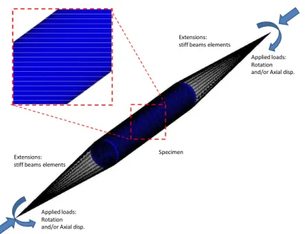
Bilinear 4 noded shell elements with 7 integration points trough thickness were employed in order to properly simulate the local buckling phenomenon occurring both in bending than in axial load testing. This type of element is particularly suitable to describe curved surfaces subjected to large strains into plastic range. Solid element could also be employed for this purpose, but shell elements were preferred due to their lower consumption of computational resource, without affecting the results. An overview of the model employed for the simulations of tests on short specimens is reported in the Figure 1. Loads have been introduced in the model at end nodes (connecting the testing machine beams frame) by application of axial forces followed by an increasing rotation up to post buckling regime. An equivalent model has been employed to simulate the tests performed on long specimen.
A dedicated sensitivity analysis on mesh size in order to obtain the optimal balance in terms of accuracy and computation resource requirements was performed before the simulation of full scale tests. It was thus decided to employ 120 elements along circumference with an axial length of 10mm.
Extensions: stiff beams elements
Extensions: stiff beams elements
Specimen
Applied loads: Rotation and/or Axial disp.
Applied loads: Rotation and/or Axial disp.
Figure 1. Overview of the FE model employed in the simulation of short column specimens
Material work hardening behaviour in terms of true stress – true stain curves, are needed as input to the model. Steel material has been characterized via tensile tests on cylindrical samples in longitudinal direction (task 3.1). The resultant curve used in finite element analysis (FEA) is reported in Figure 2. An isotropic hardening rule in combination with the Von Mises yield criterion has been adopted to describe the elastic-plastic behaviour of the CHS member deformation process.
15 0 100 200 300 400 500 600 700 800 900 1000 0 0.01 0.02 0.03 0.04 0.05 0.06 T ru e s tr e ss [M P a ] True Strain [-]
Figure 2. True stress true strain curve adopted in the FE model
Geometrical imperfections are introduced following the measured geometrical survey described in task 3.3.
D.5.2.1.2. Finite element model Main Results
Typical deformed shape and the equivalent plastic strain distribution is reported in the following Figure 3for a short specimen combined load test simulation. The plastic strain developed at compression side is influenced by the member imperfections and, as a result, buckling is driven in a position which is slightly away from the central section.
before collapse after collapse
Local buckling
Figure 3. Deformed shape and plastic strain distribution during bending process
It is interesting to notice that the maximum value of the bending moment and the corresponding rotation angle are not significantly influenced by columns imperfections like those measured on the tested products. This is shown in Figure 4 by comparing a perfect model (constant thickness, perfect cylinder) with one where measured imperfections are introduced (thickness variation, dimples and ovality). The measured residual stresses were found of negligible magnitude too (10% of yield stress) so they were not introduced in the model.
16
Figure 4. Geometrical imperfections: thickness variations introduced in the model (left) and comparison of moment vs. rotation diagrams obtained for geometrically “perfect” and “imperfect” models of long specimens
(right).
The numerical results generally show very good agreement with the experimental combined load tests: a comparison between the experimental and numerical analysis results is reported in Figure 5 where moment vs. rotation curves for the As3-50 combined load configuration are reported. Both bending moment and rotation at limit point are very well predicted by FEA.
0 50 100 150 200 250 300 350 400 0 0.5 1 1.5 2 A p p lie d B e n d in g M o m en t [k N xm ]
Rotation Axis - [deg]
AS3-50 FEM AS3-50 EXP
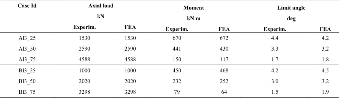
Figure 5. Comparison of experimental and numerical analysis results for the As3-50 combined load test The performed analysis resulted in the definition of M-N interaction diagrams for short and long A and B specimens. Those are graphically reported in Figure 6 and Figure 7and in Table 4 and Table 5 where both experimental and numerical results are reported.
17 0 1000 2000 3000 4000 5000 6000 7000 0 200 400 600 800 1000 1200 A xi a l L o a d [ k N ] Bending Moment [kNxm] Section A (EXP) Section A (FEM) Section B (EXP) Section B (FEM)
Figure 7. Experimental and numerical interaction diagram for long specimens of section A and B
Table 4. Summary of Experimental and numerical results for tests performed on long specimens
Case Id Axial load Moment Limit angle
kN kN m deg
Experim. FEA Experim. FEA Experim. FEA
As3 - 0 - 1112 - 6 As3-13 1340 1340 891 888 2.6 2.3 As3-25 2500 2500 732 746 1.92 1.9 As3-50 5000 5000 377 366 1.1 1.2 As3-75 7600 7600 102 104 0.42 0.48 As1 10254 10194 - - - - Bs3 - 0 - 770 - 6 Bs3-13 1000 1000 575 606 2.4 2.4 Bs3-25 1865 1865 492 482 1.81 2.1 Bs3-50 3980 3980 209 206 0.98 1.1 Bs3-75 5822 5822 76 57 0.45 0.47 Bs1 7964 7934 - 0 - 0
Table 5. Summary of Experimental and numerical results for tests performed on long specimens
Case Id Axial load Moment Limit angle
kN kN m deg
Experim. FEA Experim. FEA Experim. FEA
Al3_25 1530 1530 670 672 4.4 4.2 Al3_50 2590 2590 441 430 3.3 3.2 Al3_75 4588 4588 150 117 1.7 1.8 Bl3_25 1000 1000 450 468 4.2 4.5 Bl3_50 2020 2020 232 252 3.0 3.2 Bl3_75 3298 3298 79 64 1.5 1.9
18
D.5.2.1.3. Conclusions
Numerical analysis of the full scale tests by means of dedicated FE model developed in the commercial software MSC.MARC® have been performed.
Results show general good accordance with experimental results in terms of bending moment and rotation angle at buckling.
By means of the validated FE model, interaction M-N diagrams have been traced for sections A and B columns, extending the results of the experimental activity.
Actual geometrical imperfections measured in task 3.3 have been introduced for the simulation. Results show that the imperfections influence the plastic strain distribution during loading process but their very small magnitude has a negligible effect on the performance of the CHS members in terms of load carrying and rotational capacity up to failure.
D.5.2.2.
Numerical analysis for columns in fire condition
This section presents the numerical analysis for the columns that were tested in fire within WP4, three HSS columns (C1, C2 and C3) and one composite column (C4). The geometries and materials of the columns can be found in Deliverable 4. The thermal characteristics of the materials are presented in Appendix A. SAFIR - a finite element code, developed in University of Liege, is used as the numerical tool.
Loading
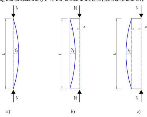
As the both values and directions of the initial deflection of the columns are unknowns, in this numerical simulation, three cases of load are considered, as the show on Figure 8
Figure 8. Noting that an eccentricity e=10 mm is used in the tests (see Deliverable D4).
a) b) c) Figure 8. Loading cases
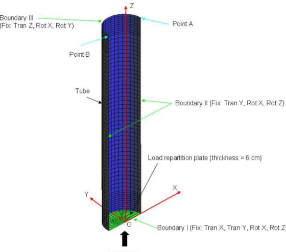
FE modeling
Both beam and shell elements are used, Table 6 and Figure 9 to Figure 13 summarize the FE modelling of the columns.
19 Table 6. Adopted FE models for the columns
Thermal analysis→ Structural analysis ↓
2D solid element (Figure 9, Figure 10, and Figure 11)
Beam element (Figure 12) Column C1, C2, C3, and C4 Shell element (Figure 13) Column C1, C2, and C3
1 1 1 1 1 1 1 1 1 1 1 1 1 1 1 1 1 1 1 1 1 1 1 1 1 1 1 1 1 1 1 1 1 1 1 1 1 1 1 1 1 1 1 1 1 1 1 1 1 1 1 1 1 1 1 1 1 1 1 1 1 1 1 1 1 1 1 1 1 1 1 1 1 1 1 1 1 1 1 1 1 1 1 1 1 1 1 1 1 1 X Y Z
Diam ond 2009.a.4 for SAFIR
FI LE: Thermal_355 NODES: 546 ELEMENTS: 450 SOLI DS PLOT FR ON TIERS PLOT STEELEC 3 FI SO 1
Figure 9. Columns C1, C2 and C3 – transversal discretization (for using beam element)
1 X
Y
Z
Diam ond 2009.a.4 for SAFIR
FILE: Shell_t_355 N OD ES: 14 ELEMENTS: 6
N OD ES PLOT SOLIDS PLOT FRON TIERS PLOT
STEELEC 3 FISO 1
20 Figure 10. Columns C1, C2 and C3 – thickness discretization (for using shell element)
1 1 1 1 1 1 1 1 1 1 1 1 1 1 1 1 1 1 1 1 1 1 1 1 1 1 1 1 1 1 1 1 1 1 1 1 X Y Z
Diam on d 2009.a.4 for SAFIR
FI LE: C_355_9 N ODES: 588 ELEMENTS: 980
SOLI DS PLOT FR ONTI ERS PLOT
STEELEC2 SILCON C_EN STEELEC3 FISO 1
Figure 11. Column C4 – transversal discretization (for using beam element)
6 2 3 4 5 1 F0 F0 7 8 9 10 F0 X Y Z
Diam on d 2009.a.4 for SAFIR
FI LE: colum n_70 NODES: 21 BEAMS: 10 TR USSES: 0 SH ELLS: 0 SOILS: 0 NODES PLOT BEAMS PLOT IMPOSED DOF PLOT POIN T LOADS PL OT
Beam Element
21 Figure 13. Columns C1, C2 and 3 – shell element discritization
Results and discussions
The fire resistances given by the numerical analysis are compared with the experimental one, the results are reported in Table 7. As an example, Figure 14 presents the deformation of the column C1 at the ultimate state, the global bucking is shown. It is observed that the numerical results are agreement with the experimental ones, in the both fire resistance and failure mode aspects.
Table 7. Comparison of the numerical results with the test results
Specimen Fire resistances given by SAFIR (in minute) Test results (in minute) Loading (a) Loading (b) Loading (c)
Shell Beam Shell Beam Shell Beam
C1 23 30 22,6 30 23,5 29 22
C2 21 22,5 21 22,5 21 21 20
C3 22 22 22 22 23 21,5 21
C4 - 104 - 104 - 84 108
The loading cases (a), (b) and (c) are described on Figure 8.
22
X Y
Z
5,0 E-02 m
Diam ond 2009.a.4 for SAFIR
FILE: hot_70 N OD ES: 1303 BEAMS: 0 TR USSES: 0 SHELLS: 1224 SOILS: 0 SHELL S PLOT D ISPLAC EMENT PL OT ( x 7) TIME: 1694 sec Shell Element
Figure 14. Column C1 (loading a, shell element) - deformation at the limit state (x7)
D.5.2.3.
Simulation data of column-base and beam-to-column joints at normal
temperature
D.5.2.2.1.
Hysteretic behaviour of both beam-to-column and column-base joints
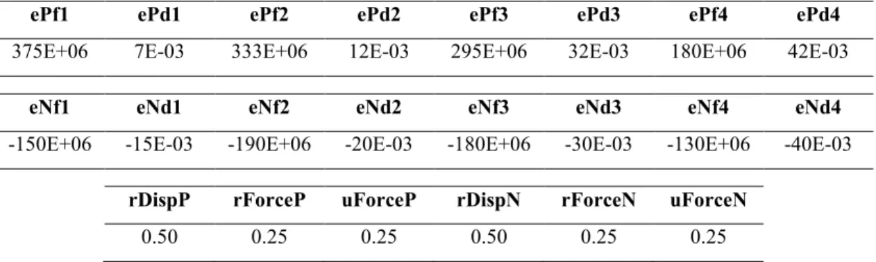
In order to investigate the response of the 5-storey prototype structure under seismic loading, it is fundamental the modelling of the hysteretic behaviour of both beam-to-column and column-base joints. The main steps were the following: i) analysis of test results to evaluate the location of plastic hinges; ii) choice of the model to take into account the behaviour, spread or concentrated plasticity; in those analyses concentrated plasticity was considered iii) choice of hysteretic models in order to simulate their actual behaviour iv) calibration of models parameters comparing numerical and experimental results. Both force-displacement of the actuator and moment rotation of plastic hinge were taken account. To calibrate the aforementioned models the whole structures tested were modelled, as shown in Figure 17, in Figure 22 and Figure 25.
Both beam-to-column and column-base joints were modeled using Bouc-Wen and pinching hysteretic models provided by Opensees, as shown in Figure 15 and Figure 16 rispectively. The two models were considered to operate in parallel, with exception of the innovative column-base joints where it was possible to model the hysteretic behaviour considering only one Bouc-Wen model. In the beam-to column joint and in the standard column-base seismic joint, the Bouc-Wen model provides the main part of actual behaviour, while the pinching model simulates slip due to damaged concrete and consequent hardening.
The calibration of the parameters took into account a unique model for the plastic hinge, in order to simulate tests subject to cyclic and random displacement protocols, respectively.
23 Figure 15. Bouc-Wen hysteretic model
Figure 16. Pinching hysteretic model
Beam-to-column joints
Experimental results summarized in the WP3 exhibited the activation of plastic hinges in weak section between the beam ends and the plates welded to the column,
Figure 17 shows the model used in numerical analysis by Opensees, to calibrate the parameters of hysteretic behaviour. The numerical model was obtained by the idealization of actual tested structure.
Figure 17. Model of tested beam-to-column joints
Figure 18 depicts the contribution of the two models used in order to simulate the hysteretic behaviour of beam-to-column joints; while Table 8 ÷ Table 10 summarizes values of model parameters.
24 Figure 18. Hysteretic models of beam-to-column joints
Table 8. Bouc-Wen parameters of beam-to-column joints
α k0 n γ β A0 δA δν δη
0.065 0.88 E+11 1.76 6927 6927 1.00 0.00 0.00 0.00
Table 9. Pinching parameters of enveloping and target points of beam-to-column joint
ePf1 ePd1 ePf2 ePd2 ePf3 ePd3 ePf4 ePd4
375E+06 7E-03 333E+06 12E-03 295E+06 32E-03 180E+06 42E-03
eNf1 eNd1 eNf2 eNd2 eNf3 eNd3 eNf4 eNd4
-150E+06 -15E-03 -190E+06 -20E-03 -180E+06 -30E-03 -130E+06 -40E-03
rDispP rForceP uForceP rDispN rForceN uForceN
0.50 0.25 0.25 0.50 0.25 0.25
Table 10. Pinching parameters of damage index of beam-to-column joint
gK1 gK2 gK3 gK4 gKLimit gD1 gD2 gD3 gD4 gDLimit
0.25 0.35 0.40 0.20 0.50 0.50 0.50 2.00 2.00 0.50
gF1 gF2 gF3 gF4 gFLimit gE dmgType
0.70 0.00 0.60 0.70 0.90 10 energy
The comparison between experimental and numerical relevant to moment-rotation relationships of plastic hinges are shown herein.
Pinching model Bouc-Wen model
25 Figure 19. Moment-rotation relationship of beam-to-column joints subjected to monotonic testing
Figure 20. Moment-rotation relationship of beam-to-column joints subjected to cyclic testing
Figure 21. Moment-rotation relationship of beam-to-column joint subjected to random testing
Table 11 collects experimental and numerical energies dissipated by plastic hinges.
Table 11. Hysteretic energy value dissipate by beam-to-column joint
Test Experimental [kJ] Numerical [kJ] Error [%]
Monotonic 19.062 19.961 4.71
ECCS 352.743 310.234 12.05
26 Standard column-base joint designed for seismic loading
This joint was modelled by the presence of plastic hinge at the base of the column in correspondence of the grout between plinth of foundation and base plate, as shown in Figure 22.
Figure 22. Model of standard column-base joint designed for seismic loading
Figure 23 depicts the contribution of the two models used in order to obtain the hysteretic behaviour of standard solution of column-base joints; while Table 12 ÷ Table 14 summarize values of parameters of models
Figure 23. Hysteretic models of standard column-base joint designed for seismic loading
Table 12. Bouc-Wen parameters of standard column-base joint designed for seismic loading
α k0 n γ β A0 δA δν δη
0.05 1.6E+11 2.00 117065.5 117065.5 1.00 0.9E-09 0.6E-09 13E-09
Table 13. Pinching parameters of envelope and target points of standard column-base joint designed for seismic loading
ePf1 ePd1 ePf2 ePd2 ePf3 ePd3 ePf4 ePd4
400E+06 3E-03 850E+06 10E-03 900E+06 50E-03 500E+06 8E-03
eNf1 eNd1 eNf2 eNd2 eNf3 eNd3 eNf4 eNd4
-400E+06 -3E-03 -850E+06 -9E-03 -900E+06 -50E-03 -400E+06 -8E-03
rDispP rForceP uForceP rDispN rForceN uForceN
0.45 0.30 -0.375 0.4531 0.30 -0.3929
Table 14. Pinching parameters of damage index – standard column-base joint designed for seismic loading
gK1 gK2 gK3 gK4 gKLimit gD1 gD2 gD3 gD4 gDLimit
0.25 1.00 1.00 1.00 0.80 0.80 0.80 0.80 0.80 1.00
gF1 gF2 gF3 gF4 gFLimit gE dmgType
27
a) b)
Figure 24 Moment-rotation relationship for standard column-base joint: a ) cyclic test; b) random test Table 15 gathers both the experimental and numerical energy dissipated by plastic hinges
Table 15. Hysteretic energy value dissipate by Standard seismic column-base joint
Test Experimental [kJ] Numerical [kJ] Error [%]
ECCS 352.011 413.118 14.79
Random 110.126 148.160 25.67
Innovative column-base joint designed for seismic loading
The joints were characterized by the presence of a plastic hinge at the base of the column in correspondence of the grout between plinth of foundation and base plate, as shown in Figure 22.
Figure 25. Model of standard column-base joint designed for seismic loading
Figure 26 depicts the contribution of the two models used in order to obtain the hysteretic behaviour of beam-to-column joint; while Table 16 summarizes the values of model parameters
Figure 26. Hysteretic models of innovative column-base joint designed for seismic loading
Table 16. Bouc-Wen parameters of standard column-base joint designed for seismic loading
α k0 n γ β A0 δA δν δη
28
a) b)
Figure 27 Moment-rotation relationship for innovative column-base joint: a ) cyclic testing; b) random testing
Table 17 compares the experimental and numerical energy dissipated by the plastic hinge.
Table 17. Hysteretic energy value dissipate by Innovative seismic column-base joint
Test Experimental [kJ] Numerical [kJ] Error [%]
ECCS 275.885 245.205 12.51
Random 83.292 112.058 25.67
D.5.2.2.1. Mechanical behaviour of a plinth relevant to an innovative seismic joint
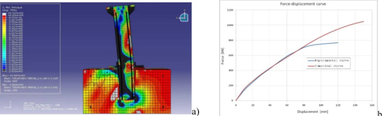
Formulae proposed in EN 1992-1-1 (2005) [8] for pocket foundations consider rectangular columns embedded in the plinth, as showed in Figure 28. The innovative solution realised by a circular column requires the investigation of Strut & Tie mechanisms that transfer forces between the column and the foundation. The analysis of the mechanical behaviour of the innovative column-base joint requires a 3D numerical model set by the ABAQUS program. The calibration of the 3D numerical model proposed required elevated computational costs due to : i) non-linearity of the problem consequent to damage of the concrete in tension; ii) presence of constrains among different parts of joints as column surface and concrete block or the base plate and the grout. Figure 29 shows the large number of rebars present in the FE model generated by ABAQUS software.
Figure 28. Plinth with a rectangular column Figure 29. Re-bars in the FE model of a column-base joint Analyses were conducted with FE program ABAQUS by means of a Standard Analysis. Column-base were subject to cyclic tests only; therefore, the envelope of force-displacement relationship was considered. The model was calibrate applying monotonic displacement and comparing: i) the horizontal force provided by FE model with the one recorded by the actuator in order to apply the same
29 displacement during tests, as shown in Figure 30; ii) the forces recorded during the test by strain gauges welded on the rebars located in the plinth.
Numerical results were satisfactory and in agreement with experimental data till the onset of yielding. After the yielding the numerical response showed higher stiffness w.r.t. actual response. It was very difficult to take account in the model the damage of the grout owing to cyclic loading, between the steel column and the foundation block.
a) b)
Figure 30. Innovative column-base joint: a) distribution of stresses in the specimen; b) comparison between numerical and experimental data
The resulting mechanism was endowed with: i) two frontal struts along the diagonal of the plinth with a rectangular section of about 400 x 360 mm; ii) a rear strut parallel to the face of the plinth with a rectangular section of about 500 x 400 mm. Figure 31 shows the geometry of the struts in the plinth obtained by means of FE analysis.
Figure 31. Strut & tie mechanism and distribution of compressive principal stresses for the plinth of the innovative column-base joint
D.5.2.4.
Numerical analysis of connections in fire condition
This section presents the numerical analysis for the connections (beam-to-column joints and column bases) that were tested in WP4. The detail of the geometries and the materials of the specimens and also the test descriptions (location of thermocouples, location of displacement transducers, loading sequences, etc.) can be found in Deliverable D4. It concerns two static joints (J11 and J12), two seismic joints (J21 and J22), one static column base (CB1) and two seismic column bases (CB2, CB3).
Thermal analysis for static joints
In the fire condition, it can say that the critical zones of the static joints are the bolts, plates and the columns, not the rebar that are protected by the concrete. Moreover, there are not much influences of the slap to the temperature development in the steel parts (bolts, plates and column).By consequence, the use of 3D solid model for the whole of joints (Figure 32) may be not necessary, as it is expensive in the level of computation cost. In order to simulate the temperature in the “bolt” zone, the model as the show on Figure 33 can be adopted. The 2D model on Figure 34 may be used for the vertical plate and the column. Using the ISO FIRE in the model, the temperature development in the different zones given
30 by proposed models are compared with the test ones (Figure 35 to Figure 38). The agreements are shown and it point out that the used models (Figure 33 and Figure 34) can be applied to simulated temperature in the static joints under fire loading.
Figure 32. Static joint - 3D model in thermal analysis for the whole of static joints
Figure 33. Static joint - 3D model for the “bolt” zone
31
Temperature in vertical plate (outside part)
0 100 200 300 400 500 600 700 800 900 0 5 10 15 20 25 30 35 40 45 50 55 Time (minute) T e m p e ra tu re ( d e g re e ) SAFIR Test_J11_th6 Test_J12_th6 Test_J11_th8 Test_J12_th8
Figure 35. Static joint – comparison of temperature in the vertical plate (outside part)
Temperature in vertical plate (inside part)
0 100 200 300 400 500 600 700 800 0 5 10 15 20 25 30 35 40 45 50 55 Time (minute) T e m p e ra tu re ( d e g re e ) SAFIR Test_J11_th7 Test_J12_th7
32
Temperature on the column
0 100 200 300 400 500 600 700 800 900 0 5 10 15 20 25 30 35 40 45 50 55 Time (minute) T e m p e ra tu re ( d e g re e ) SAFIR Test_J11_th5 Test_J12_th5 Test_J11_th9 Test_J12_th9
Figure 37. Static joint – comparison of temperature in the column
Static joint: Temperature in "bolt" zone
0 100 200 300 400 500 600 700 800 900 0 5 10 15 20 25 30 35 40 45 50 55 Tim e (minute) T e m p e ra tu re ( C . d e g re e ) SAFIR Test_J11_th1 Test_J12_th1 Test_J11_th2 Test_J11_th3 Test_J11_th4 Test_J12_th4 Test_J12_th2 Test_J12_th4
Figure 38. Static joint – comparison of temperature in the “bolt” zone
Thermal and mechanical analysis for seismic joints Thermal analysis
A 3D solid model (Figure 39) is developed to simulate the temperature in the steel parts (beam, bolts and plates) of the seismic joints. On the other hand, 2D model is adopted to predict the temperature in
33 the rebars of the concrete slap (Figure 40). In the practices, the steel parts may be grouped into three zones (Figure 39), the differences of temperature within each zone can be neglected.
The numerical results are comparison with the experimental ones (Figure 41 to Figure 44). In general, the temperatures given by the numerical analysis are greater than the one of the tests, in particular with respect to the temperature in the rebar. The reason is maybe the influence of the composite column (absorb much of energy) that is not modelled in the model. However, the numerical analysis gives the conservative side.
Figure 39. FE modelling of the seismic joints in the thermal analysis
34
Seismic joint: Temperature in zone 1
0 100 200 300 400 500 600 700 800 900 1000 0 5 10 15 20 25 30 35 40 45 50 55 60 Time (minute) T e m p e ra tu re ( C d e g re e ) SAFIR_zone 1 Test_J21_th16 Test_J21_th17 Test_J21_th12 Test_J21_th19 Test_J22_th16 Test_J22_th18 Test_J22_th19
Figure 41. Seismic joint – comparison of temperature in zone 1
Seismic joint: Temperature in zone 2
0 100 200 300 400 500 600 700 800 900 1000 0 5 10 15 20 25 30 35 40 45 50 55 60 Time (minute) T e m p e ra tu re ( C . d e g re e ) SAFIR_Zone2 Test_J22_th7 Test_J22_th12 Test_J21_th7 Test_J21_th18
35
Seismic joint: Temperature in zone 3
0 100 200 300 400 500 600 700 800 0 5 10 15 20 25 30 35 40 45 50 55 60 Time (s) T e m p e ra tu re ( C . d e g re e ) HEB280_F2 Test_J21_th5 Test_J22_th5
Figure 43. Seismic joint – comparison of temperature in zone 3
Seismic joint: Temperature in the rebars
0 50 100 150 200 250 300 350 400 450 500 0 5 10 15 20 25 30 35 40 45 50 55 60 Time (minute) T e m p e ra tu re ( C . d e g re e ) SAFIR_Rebar2 SAFIR_Rebar1 Test_J21_th20 Test_J21_th21 Test_J22_th20 Test_J22_th21
Figure 44. Seismic joint – comparison of temperature in rebars
Mechanical analysis
It is complicated to use 3D solid model for simulating the mechanical behaviour of the joints, so a model by using beam elements is proposed (Figure 45). In this model, the section of beams is varied according to the actual configuration of the joints, the shear deformation of the bolts are omitted. The temperature developments recorded by the thermocouples in the tests are used to impose the temperature in the corresponding zones of the sections.
The load point displacements given by SAFIR are presented on Figure 46 and Figure 47 which are compared with the experimental ones (Figure 48 and Figure 49). It can observe that the fire resistance is good in agreement between the calculation and the tests. However, the time-displacement curves are more ductility than the numerical ones.
36 Figure 45 . Mechanical modelling of the seismic joints
Seismic joint (J21): displacement given by SAFIR
-30 -25 -20 -15 -10 -5 0 5 0 5 10 15 20 25 30 35 40 45 50 55 60 65 70 75 Time (minute) D is p la c e m e n t (m m )
37
Seismic joint (J22): displacement given by SAFIR
-35 -30 -25 -20 -15 -10 -5 0 0 5 10 15 20 25 30 35 40 45 50 55 60 Time (minute) D is p la c e m e n t (m m )
Figure 47. Seismic joint J22– point load displacement given by SAFIR
Seismic joint (J21): Comparison of displacement
-120 -100 -80 -60 -40 -20 0 20 0 5 10 15 20 25 30 35 40 45 50 55 60 65 70 75 Time (minute) D is p la c e m e n t (m m ) J21_test SAFIR
38 Seismic joint (J22): comparison of displacement
-120 -100 -80 -60 -40 -20 0 20 0 5 10 15 20 25 30 35 40 45 50 55 60 Time (minute) D is p la c e m e n t (m m ) SAFIR Test
Figure 49. Seismic joint J22–comparison of displacement
Thermal and mechanical analysis for column bases Thermal analysis
Figure 50 and Figure 51 are respectively shows the developed model for CB2 and CB3. For the moment, the temperatures in some zones given by the FE model are compared with the test results (Figure 52 and Figure 53), the agreement is shown.
Noting that the thermal analysis results for the end plate and the bolts of CB3 can be used for CB1 (static column base) while the temperature in the steel column of CB1 may be computed as in the isolated steel column in taking into account the influence of the foundation..
39 Figure 50. EF modelling in thermal analysis of column base CB2
40 CB3: temperature in rebar 0 20 40 60 80 100 120 140 0 300 600 900 1200 1500 1800 2100 2400 Time (s) T e m p e ra tu re ( C . d e g re e ) SAFIR Test_CB3_th2 Test_CB3_th5 Test_CB3_th6
Figure 52. Seismic column base - comparison of temperature in rebar
CB3: temperature in tube 0 100 200 300 400 500 600 700 0 300 600 900 1200 1500 1800 2100 2400 Time (s) T e m p e ra tu re ( C . d e g re e ) SAFIR Test_CB3_th1 Test_CB3_th3 Test_CB3_th7
Figure 53. Seismic column base - comparison of temperature in steel tube
Mechanical analysis
In the fire condition, after about 30-40 minutes, it can say that the capacities of steel parts (stiffeners, end plate and bolts) strongly decrease, while the composite column can resist in more of time. Therefore, the behaviour of the column bases is quite similar to the behaviour of the composite column clamped in the foundation (Figure 54). This observation is in agreement with the experimental tests:
41 CB2 and CB3 are very different in the level of steel parts (end plate thickness, number of bolts and present of stiffeners), but the behaviour in fire are similar (Figure 55 and Figure 56). Noting that CB2 and CB3 were tested under the same condition (as ISO fire, test set-up and load value). From the remark, the model using beam element (end plate, bolts and stiffeners are neglected, only composite column is considered) is proposed to simulate the tests on CB2 and CB3 specimens (Figure 57). In this model, the temperature in the tube and the rebar are imposed by the temperature recorded by the thermocouples. The time-displacement curves given by the SAFIR is reported on Figure 58 (SAFIR_V is the vertical displacement of point C while SAFIR_H is the horizontal displacement of the point E, see Figure 57). The fire resistances of the column bases are well predicted by the present model while the time-displacement curves of the tests are more ductility than the numerical one (Figure 59).
Figure 54. On the resistance in fire of column base with composite column
42 Seismic joint: displacement observation
0 50 100 150 200 250 300 350 400 450 0 600 1200 1800 2400 3000 3600 4200 4800 5400 6000 Time (s) D is p la c e m e n t (m m ) CB3 CB2 CB2_2
Figure 56. Total displacement given by tests (similar for CB2 and CB3)
43 -30 -20 -10 0 10 20 30 40 0 1000 2000 3000 4000 5000 6000 Time (s) D is p la c e m e n t (m m ) SAFIR_V SAFIR_H
Figure 58. Displacements given by SAFIR
-150 -100 -50 0 50 100 150 200 0 1000 2000 3000 4000 5000 6000 Time (s) D is p la c e m e n t (m m ) CB3_V CB3_H CB2_V CB2_H SAFIR_V SAFIR_H
44 Concluding remarks
From the numerical results, the following remarks can be drawn for the moment:
• The 2D model can be used to calculate the temperature development in the rebars of the slap and in the vertical plate of the static joints while 3D model is recommended for the other components. The parametric study on the temperature developments are needed such that the simple guidelines can be given, this is a future perspective of the work.
• The beam elements can be used in the mechanical analysis for seismic joints and seismic column bases. In the seismic joints, the beam sections should be varied according to the actual configuration of joints. With respect to the column base, the influences of the end plate, the bolts and the stiffeners to the fire resistances may be neglected, the fire resistance of the column bases may be considered as the composite column one.
D.5.2.5.
Numerical analysis for vertical plate of static joints
This section presents the numerical study on the “vertical plate” component of the static joints. The static joints were tested in fire condition within WP4 while four (3) “vertical plate” components were tested at the normal temperature in WP3.
Notices (Figure 60)
t: thickness of the plate; h: height of the plate;
b: width of the plate part outside the tube; D: inside diameter of the tube;
FEd: design value of the horizontal component of the load;
VEd: design value of the vertical component of the load;
α: load direction; E: Young modulus; υ: Poisson ratio.
Figure 60. Beam-to-column joints - through plate component
General considerations and hypotheses
Figure 61 describes the buckling mode of the whole joint while the buckling mode of the through plate is shown on Figure 62.
45 Figure 61. Buckling mode of joint
Figure 62. Buckling mode of through plate
For the simplification reason, the through plate is devised into two parts, inside part (inside the column) and outside parts (outside the column) with the boundary and loading condition as the show on Figure 63. The buckling theory of plate is applied to study the strength of each part.
46 Figure 63. Modelling of boundary and loading for the through plate
Using the buckling theory of plates, the buckling stresses of the inside and outside parts can be written by the following equations:
2 2 , 1 2 12(1 ) c ou E t b
π
σ
µ
ν
= − ; 2 2 , 2 2 12(1 ) c in E t hπ
σ
µ
ν
= − . Numerical investigationThe coefficients µ1 and µ1 in above equations are used to take into account boundary condition, loading
condition, plasticity and initial imperfection. In this work, these coefficients are determined by the numerical analysis, as:
2 2 1
(
,)
/
212(1
)
c ou numericalE
t
b
π
µ
σ
ν
=
−
; (D.5.2.5.1) 2 2 2(
,)
/
212(1
)
c in numericalE
t
h
π
µ
σ
ν
=
−
, (D.5.2.5.2)with σnumerical is calculated by LAGAMINE (a nonlinear finite element code developed in University of
Liege) considering the boundary condition, the loading, the plasticity and the initial imperfection, as the description on Figure 64 and Figure 65. In the numerical models, 3D solid elements are used.
47 Figure 65. Material modelling in the numerical analysis
In order to validate the FE model, some examples existing in the literature [14] are examined, as the following.
Problem 1: simple supported, square plate under uniaxial load [14]. Elastic modulus E=10,700 ksi, yield strengthσ0=61.4 ksi. In [14], Ramberg-Osgood material / 0/ ( 0/ )
c
E k E E
ε σ= + σ σ with c=20 and k=0.3485 is applied while the material described in Figure 65 is adopted in LAGAMINE. The initial imperfection 1/200 as the recommendation of Eurocode 3, part 1-5 (on plated structures) is adopted (Figure 66). The comparison of the results is presented in
Table 18 18. The buckling stress given by LAGAMINE is closed with the Bleich’s one.
Figure 66. Problem 1: a) plate outline b) initial imperfection used in LAGAMINE; c) FE modelling in LAGAMINE; d) Buckling mode given by LAGAMINE
48 Table 18. Problem 1 - Comparison of results
b/t Buckling stress (in ksi)
IT DT Bliech’s theory LAGAMINE
22 70.844 60.080 56.125 51.460 23 65.166 58.836 55.139 50.366 24 60.713 57.397 54.109 49.258 25 57.363 55.730 52.988 48.090 26 54.598 53.806 51.712 47.289 27 51.938 51.569 50.185 46.520 28 49.112 48.962 48.269 45.642
Problem 2: A quite thick plate is considered in this example. Free-Simple-Free-Simple square plate under uniaxial plate was studied by Wang et al (2001) [14] with the variation of thick/wide ratio and also the Ramberg-Osgood parameters are varied.
49 Figure 67. Problem 2: a) plate outline b) initial imperfection used in LAGAMINE; c) FE modelling in
GAGAMINE; d) Buckling mode given by LAGAMINE
Table 19. Problem 1 - Comparison of results
Buckling stress factor 2 2
/( ) ctb D σ π E/σ0 IT DT LAGAMINE 200 1.136 0.999 0.966 300 1.104 0.819 0.686 500 1.104 0.473 0.434 750 1.104 0.298 0.215
The results given by LAGAMINE are closed with the DT one. It can say that in this case the buckling stress factors coming from IT are not reasonable because they don’t change when yield strength varies. The present model is used for the present case (vertical plate of static joints) with the modification of boundary conditions (Figure 63). The parametric study (the geometric dimensions of the plate are varied such that almost practical case can be coved) is performed, and the corresponding values of µ1
and µ1 are obtained (the detail values can be found in Deliverable 6).
D.5.2.6.
Numerical analysis for “end plate” component of static column bases
One static column base was tested at normal temperature under cyclic loading in WP3, and one same configuration of the column base was also tested in fire condition within WP4. Moreover, three (3) “end plate” components were tested at normal temperature under monotonic loading in WP3. This section presents the numerical investigation for the “end plate” components. The details on the geometrical and mechanical properties of the investigated components can be found in Deliverable D3.
Numerical strategy
A finite element model has been developed, using a homemade finite element model called LAGAMINE able to reflect the full non-linear behaviour of elements subjected to large deformations, in order to simulate the behaviour of the joints. The main features of the proposed numerical model may be summarized as follows (Figure 68):
• 3D solid element are used;
• Agerskov’s conception for the bolt shank length (see Agerskov (1976)) is adopted (Figure 69 and Table 20)
• Plastic nonlinear material is introduced with the natural curve that is established from nominal curve given by the coupon tests (see Deliverable 3).
• Geometrical nonlinearities (large deformation) are taken into account;
• Contact between the joint components (bolts-flanges, flange-flange) is modelled;
• Geometry of the weld is introduced (but the weld material is assumed to have the same properties as the tube steel);
50 • The bolts in the compression zone is not considered;
• The geometries of the investigated specimens are presented in • Table 21.
Figure 68. FE modelling for “end plate” component
Figure 69. Geometries of the bolts
Table 20. Detail value of bolt geometries (Figure 69)
Bolts Ab (mm2) As (mm2) tf (mm) lh (mm) ln (mm) ls (mm) lt (mm) lw (mm) dw (mm) leff (mm) Specimen 1 707 566 14 18.5 23.7 41 5 18 56.5 65,1
51
Specimen 2 707 566 16 18.5 23.7 41 0 9 56.5 52,9
Specimen 3 707 566 18 18.5 23.7 41 4 9 56.5 57,5
Table 21. Geometries of the investigated specimens
Specimen Geometries (mm) Material strength (N/mm2)
b h tp d e1 e2 w a fy fu
1 400 400 14 193.7 60 60 23.685 16 418 602
2 400 400 16 193.7 60 60 23.685 16 418 602
3 400 400 18 193.7 60 60 23.685 16 418 602
Results
The deformation and the load-displacement curves given by the numerical analysis are compared with the experimental one. The deformation is in good agreement (Figure 70) while the difference about 10% for the load-displacement curves (Figure 71 to Figure 73).
52 Figure 70. “End plate” component – comparison of deformation
Specimen 1: comparison of displacement
0 10 20 30 40 50 60 70 80 90 100 0 20 40 60 80 100 120 140 160 180 200 Displacement (mm) M o m e n t (k N ) Test LAGAMINE