Application of Hough Transform for Seed rows Localisation using
Machine vision
V. Leemans ; M.-F. Destain
Gembloux Agricultural University – Unité de mécanique et construction
Passage des Déportés, 2 – B 5030 Gembloux, Belgium ; e-mail of corresponding author : [email protected]
1. Abstract
This paper compares two methods based on machine vision to provide driver assistance in seed drill guidance in order to improve spacing accuracy during contiguous passages.
The first case consisted of following the furrow created at the preceding passage by a special marker disc attached to the seed drill. A camera was located on the tractor and detected this furrow. In the second case, the seed rows themselves were detected by the camera without making use of the marker disc.
In both cases, several video sequences were acquired in various situations, including different soil textures and various illumination conditions (375 sequences were acquired during three years). A pre-treatment of these sequences was performed and included a background subtraction in order to remove shadows and other wide unevenness. In the first case, the best results were obtained by using an image treatment based on the Hough transform coupled to a recursive filter. The search of the maximum of the Hough transform was performed using a mean shift algorithm. In the second case, where several parallel rows were simultaneously present on the images, an adapted Hough transform was proposed which took into account the a priori knowledge of the rows spacing. The trueness and precision in row detection were superior in the second case. The results are compatible with the application, since the trueness was smaller than 30 mm. This suggested that it can be possible to assist the manual guidance of a seed drill by an automatic system consisting in a
camera detecting the seed rows.
Key words : guidance, Hough transform, mean shift, precision seed drill, machine vision, sugar beet.
2. Introduction
The guidance of the seed drill is obtained by steering the tractor. A furrow created by a disc in the soil, during a previous passage have to be followed to ensure a correct lateral position. Currently, this guidance is entirely undertaken by the tractor driver therefore some variation in the spacing between two contiguous passages may occur.
Historically, the harmonisation of the sugar beet production leaded to machines of six row widths or of multiples of six rows. The seed drill often comprises twelve rows and the harvesting machines six rows. The development of height-row harvesting machines would increase the productivity and reduce the harvesting costs. These new versions of harvesters must therefore operate within plant rows corresponding to adjacent passages of the seed drill with slightly varying spacing. The current solution consists of mounting pairs of harvest shares on independent frames to allow a certain clearance between pairs of rows. However, the driving precision required during the sowing demands a constant concentration from the tractor driver during the seed drill operation, increasing susceptibility to fatigue and consequently decreasing productivity.
This paper addresses the problem of assisting the guidance of a seed drill in order to control the distance between contiguous passages. This work was performed in two ways: detection of the furrow created by a disc during the previous passage and detection of the seed rows themselves.
agricultural machines, using a combination of existing solutions including global positioning, inertial sensors, odometers and computer vision (Jahns, 2000; Pilarski et al., 2002). Stoll and Kutzbach (2000) presented a guidance system for a self-propelled windrower using a real time kinematic global positioning system, but most devices for precise driving assistance of agricultural machines are mainly based on simpler, cheaper systems such as machine vision.
No studies were found about a guidance system based on the detection of furrow or on seed rows. Guidance systems based on computer vision in agriculture are mainly used for cut edge and plant rows detection. The similarities between these researches and the task presented in this paper are presented here after.
To distinguish between cropped and uncropped zones in images Debain et al. (2000) used grey level and texture information. Pilarski et al. (2002) tracked the cut crop line edge by adjusting each row of the image with a step function, initially arbitrarily chosen and then determined by computing Fisher’s linear discriminant function on the previous image. Benson et al. (2003) localised the cut edge of maize during harvesting by first determining whether or not the cut edge was shadowed and then localising the edge using an adaptive threshold.
Considering the problem of crop row detection, Pla et al. (1997) based an algorithm on the detection of the vanishing point of the row cluster. This technique was borrowed from road vehicle guidance and the authors stated that compared with other applications, the ‘natural’ environment is characterised by irregular and undefined shapes with a high texture content. The processing of the images included the segmentation of the colour images, the computation of the row skeletons, the localisation of straight lines, the tracking of the vanishing point and the extraction of information from the lines concurring to the vanishing point. However, this technique was computationally demanding. Tillett and Hague (1999) described a method to track rows of cereals. The images were segmented by ‘thresholding’
and the position of the rows was given by applying the Hough transform. Marchant (1996) used a similar technique tested on cauliflowers, sugar beet and widely spaced double rows of wheat and showed how considering several rows simultaneously increased the robustness of the algorithm. Tillett et al. (2002) exploited the periodic variations of luminance between the soil and the plants due to the parallel crop rows. A filter was applied which allowed the frequency of the crop rows to be extracted whilst attenuating the lower frequency effects of shadows and higher frequency effect, due predominantly to weeds. Søgaard and Olsen (2003) used an original method for double spaced wheat row localisation. The grey level images were divided in horizontal strips and each strip into sub-strips having a width corresponding to the inter-row width. The gravity centre of the mathematically enrolled mean sub-strip gave, for each strip, the position of the rows and an estimation of the relative accuracy. The estimation of the offset and of the orientation was given by weighted linear regression for the image. The procedure was stated to reduce computational time.
One of the problems encountered in outdoor image acquisition is the unevenness of the lighting conditions, in time and space. The variations of the sun elevation and the nebulosity contribute to change the global illumination of the scene observed by the camera. The presence of shadows is due to illuminations variations within the image. The variations from one image to the other could be partly compensated by the camera itself or by adjusting threshold levels with the mean grey level of the image (Tillett & Hague, 1999) or by developing robust algorithms (Tillet et al., 2002 ; Søgaard & Olsen, 2003). The problem of the shadows should be considered carefully. Pilarski et al. (2002) developed an empirical shadow compensation algorithm. Onyango and Marchant (2001) proposed a colour image (red, green, blue) to grey level image transformation to eliminate the effect of the shadows, computed using the spectral characteristics of the irradiance and of the objects (soil and plants).
detection of soil furrows or seed rows (the traces), described in this paper. Compared with edge detection, the traces are narrow elements which present dimensions similar to the clods responsible for the image texture. In contrast to plant row detection, the traces and the surrounding matter (the rest of the field) are of the same nature, differing only by mean luminance or texture but not by hue. Furrow detection implies the detection of a single trace in the image rather than several rows. For the seed rows, as the traces are quite narrow, the camera must be placed close enough to them.
Two methods for the detection of the furrow were studied, the first one that used the Hough transform was inspired by the works of Marchant (1996) and of Tillet and Hague (1999). The second one was based on the division of the image into several strips following Tillet et al. (2002) and Søgaard and Olsen (2003). To localise the seed rows, the basic concept was to detect several rows simultaneously by using an adaptation of the Hough transform.
The objective of this paper is to select the most suitable method to be used in a seed drill automatic guidance system: furrow detection or seed rows recognition.
3. Materials and methods 2.1. Material
Video sequences were acquired during three sugarbeet sowing seasons, from Spring 2002 to Spring 2004. In 2002 and 2003, 326 videos of the furrows were acquired by a camera fixed on the tractor, which represent around three hours an a half and about 12 km covered. In 2003 and 2004, 49 videos of the seed rows were acquired, which is around two hours and 7.5 km wandered. The camera was fixed to the seed drills beyond the left extremity of the machine, in such a way that at least two rows could be observed.
Many parameters, such as the lighting (direct sun or light diffused by clouds, elevation of the sun), the soil humidity and the dimensions of the clods change the luminance and the
contrast in the image and may thus affect the way the algorithms operate. In order to encounter this variability, the experiments took place in two regions in Belgium, differing by the climate and the soil (Hesbaye, with deep silty soils, rather flat relief and an altitude around 150 m and Condroz with sandy-clay soil sometime cobbly, varied relief and an altitude around 250 to 300 m which usually induces a delay of one to two weeks in the beginning of the seeding period, compared with Hesbaye). The videos were acquired during the whole seeding period. However, as the soil have to be sufficiently warmed-up and sufficiently dry to able to drill, the weather was always clement. Sunny conditions with morning fog or mist and drying soils were most encountered.
An inexpensive universal serial bus (USB) camera Philips PCVC 740K (Koninklijke Philips Electronics N.V., Eindhoven, the Netherlands) was used in 2002 and 2003. A Unibrain Fire-iA400 1394 camera (Unibrain S.A., Athens, Greece) equipped with a lens having a focal length of 6 mm was used in 2004. Both were colour mono-charge coupled device (CCD) cameras. It was a fix aperture for the USB camera and the aperture of the lens of the Unibrain camera was set manually. The built-in automatic control of the electronic shutter were found suitable for the application.
The commercial camera (Philips PCVC 740K) was chosen for its performances and its low cost. This camera enable numerical video sequences to be produced with a resolution of 320×240 pixels, at a rate of 30 images per second, in various lighting conditions. Its main drawback was the poor optics which caused some ‘vignetting’ (darkening of the border of the image). This aspect was easily corrected by an image treatment (background subtraction, see section 2.2.1.).
The cameras were placed looking downwards, with their optical axis having an angle of 30° with the vertical, in the forward direction. The distance between the soil and the camera was of 0.9 m for the five first measurement places and of 1.2 m for the others. The cameras were plugged on the USB or on the IEEE 1394 port of the computer. The programs used for
the images treatments and the post-treatments were written in C++ using gcc (Free Software Foundation, Inc.). The central processing unit was a ‘Pentium III’ (® Intel Corp.) having a clock frequency of 667 MHz. The video sequences were saved as audio video interleave (AVI) files.
2.2. Detection of the furrow
2.2.1. The Hough transform based method
The Hough transform is widely used for localisation of linear objects in images (Sonka et
al., 1993). This transform is quite robust against ‘noise’ and missing parts (the result of the
algorithm is only slightly sensitive to imperfect data or to interferences), but limitations can be encountered when the ‘noise’ becomes important compared with the contrast of the objects and when lures are present in the images. In these situations, the detection of the maxima corresponding in the Hough space to the rows in the image could become a difficult task. The studied application presents those characteristics. Indeed, in the detection of seed rows, variations in the soil relief induce differences in the irradiance and consequently clods or tillage furrows add high uncertainty (the ‘noise’).
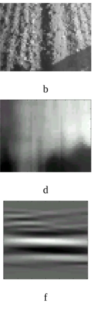
The Hough transform computes uni-dimensional integrals of the image in a given number of directions. The result is a new image (the ‘Hough space’, one dimension for the position perpendicularly to the integration direction, noted r and one for the angle, noted α) where the position of straight lines appears as maxima. The classical pretreatment of the Hough transform consists of revealing the limit of the objects and applying a threshold in order to obtain bi-level images. The objective of this research was to localise linear elements rather than to find the limits of objects. Consequently the pretreatments had to make the lines visible by removing unnecessary information, unwanted noise (clods) or the shadows of neighbouring objects (such as trees, the tractor or the camera). The results of the pretreatments were grey level images, not bi-level images. Figure 1 shows each step of the pre-treatment, the result of the transformation and the result of the detection.
Because the hue and the saturation of the soil was uniform in the images, the information in the three colour channels were redundant and only the data of the green channel were used (Fig. 1a). The images were acquired with a size of 320×240 pixels. The furrow was about 100 mm (30 pixels) wide and the clods were far smaller. As a smaller image contained sufficient information and generated a smaller computational load, the size was reduced, the scaling coefficient being adjusted (Fig. 1b). Aliasing effect was avoided by applying a Gaussian convolution filter. After the reduction, another Gaussian filter was applied in order to remove high frequencies (Fig. 1c). The size of the second filter was adjusted. The shadows and other wide unevenness were then removed using a background subtraction. The background was first obtained by applying a median rank filter on the pre-treated image. The median filter is well suited to remove spikes and thin lines while leaving the edge of the objects non blurred (Fig. 1d). Subtracting the background from the pre-treated image revealed the trace, as shown in Fig. 1e. This method was efficient for shadows larger than the furrow. The size of the median filter was thus a compromise. Values varying from 5 to 13 pixels were considered. A larger filter was able to reveal larger traces, but also left larger shadows and was more computational demanding.
As the angle between the trace and the moving direction remained small, the angles of the integration directions were limited between -π/12 and π/12, with 48 steps. The position of the trace was given by the maximum of the Hough transform and then by computing the position at the bottom of the image. The considered maximum was the absolute maximum. A variant for the selection of the maximum was used, in order to identify and try to avoid the lures. All the local maxima were researched by the mean shift algorithm proposed by Cheng (1995). The basic principle is to consider a set of point in the Hough space. The mean value of the Hough transform is computed on an area around each point, and each point is shifted to this mean position. These two steps, computation of the mean and shifting, are repeated up to the convergence of each point to a local maximum. The points
reaching the limit of the Hough subspace, corresponding to lines at the limit of the image or presenting an angle of -π/12 and π/12 were ignored. One of these maxima was then selected taking into account one or a combination of three parameters: the distance with the maxima extracted from the previous image, the highest maxima, the maxima presenting the highest volume i.e. the one to which the most point have converged.
The Hough transform based method was found too slow to treat the videos at 30 images per second. As the speed of the tractor during the sowing was about 1 ms-1 and as the
lateral movements were relatively small, a slower rate was considered and the behaviour of the algorithm was tested with one image out of five (equivalent to an acquisition frequency of six images per second).
2.2.2. Profile and regression based methods
The Hough transform requires as many uni-dimensional integrations of the image as there are angle steps in the resultant image (48 in our case). Another method was developed with the objective of reducing the computational time. This method required the equivalent of one integration. Moreover, the pre-treatments were applied on one dimensional profiles, which contributed to reduce the computational load.
The furrow appeared on the images as an almost vertical band (Fig. 1a). Because of the small portion of ground observed by the camera and the large radius require by the seed drill to turn, the direction changes did not produced visible curvature in the images. The image was divided horizontally into n strips, and each strip vertically integrated into a mean profile which was then pre-treated in a similar way as the images (Fig. 2). The size reduction and the original profiles were computed in one step, the luminance attributed to a point of a profile being the mean value of the area covered by this point on the image. This was sufficient to avoid any aliasing effect. An uni-dimensional Gaussian convolution filtering was applied to remove minor interference from clods, amongst other sources (Fig. 2). Similarly, a uni-dimensional median rank filter was applied to the profile to remove peaks
and troughs. It must be noted that the ‘standard deviation’ of the Gaussian filter was considerably smaller than the width of the median filter. Those two parameters were adjusted. The difference gave the flattened profile, where the general trends and the shadows had vanished, but where the peaks corresponding to the traces remained.
After having extracted the minimum in each profile (represented by the dot in Fig. 2), a straight line was then adjusted by regression and the position was computed at the bottom of the image.
2.3. Detection of the seed row
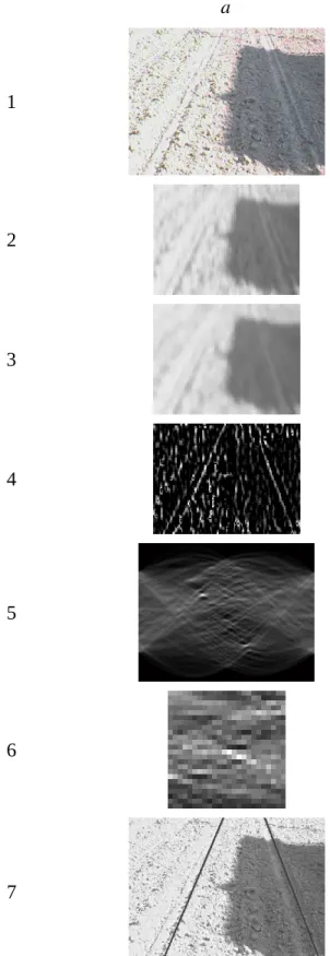
The passage of the seed drill leaves a trace on the soil presenting a flat profile of about 0.06 m width, with a small hollow in its centre. For each row, the central hollow as well as one boundary of the flat profile were usually visible on the images as thin dark lines on a bright background (Fig. 3).
The pretreatments presented in Fig. 3 were the same as for the detection of the furrow. The trace left by the seed drill is narrower than the furrow and the value of the parameters were adapted. The size of the image was reduced to various sizes from 120×90 pixels to 60 ×60 pixels. Square and rectangular Gaussian filters of various dimensions were also tested. Several sizes of the median filter were considered (varying from 3 to 11 pixels width).
As long as the geometry of the acquisition (height and tilt angle of the camera, focal length) is not modified, the distance and the angle between the projection of lines in the image remain constant, even if the camera move horizontally. In order to detect the cluster of lines in one operation, one transform was carried out for each line, but with different angular and lateral references, so that the maximum representing each line was positioned at the same point of the Hough space. The transforms were carried out for angles comprised in an interval of 0.6 radian centred on the reference angle of the considered line and for a width given by :
wHT wi nrow 10 (1) where: wHT is the width of the part of the image to which the Hough transform was
applied; wi is the width of the image; nrow is the number of rows in the cluster. The values of
each part of the transform were summed. The maxima corresponding to the crop row were added, while others peaks resulting for example from the tillage were added to the ‘noise’ and thus diluted. When the seed drill was correctly positioned, the coordinate of the maxima was at (0,0), which corresponded to the centre of the Hough space image.
2.4. Post processing
The results from the image treatment were quite noisy and could not be used directly to command the displacement of a seed drill. Two methods were used to filter the data, the Kalman filter and a non linear recursive filter.
The Kalman filter (presented originally in Kalman, 1960) is a Bayesian estimator of the position provided that the movement of the seed drill and the measurement could be given by:
xk Axk 1 Buk wk, x , w n, u l (2)
zk Hxk vk, z m (3)
where: xk, xk-1 are the state vector at time step k and k-1, respectively; zk the measurement; uk
is the displacement imposed by the regulation; wk was the process white noise (this noise is
supposed to present no correlation between its value at a time step and any previous time steps) having a Gaussian distribution with a null mean and a covariance matrix Q; vk is the
measurement white noise having a Gaussian distribution with a null mean and a covariance matrix R. The values of Q and R were estimated thanks to the reference presented below (2.5.; the reference was considered as the true value of xk). As there was no regulation on
the lateral displacement of the seed drill, uk was always zero and B was not necessary. The
is the abscissa of the furrow at the bottom of the image. The estimation of the actual position and its best estimation based on earlier data is the previous positions xk-1 , thus A=1
and the measurement of the position is correct and unbiased, thus H=1. For the detection of the seed rows, xk was the estimated Hough space coordinates:
xk r
k (4)
and zk was the measured Hough space coordinates:
zk r
k (5)
where: r and r are the position perpendicularly to the integration direction (respectively estimated and measured), and and α are the angle of this direction with the vertical in the image (idem). The measurement came directly from the detection of the maximum in the Hough space and the variables r and α where considered independent respectively to each other. Matrices A and H where thus equal to the two dimensional unity matrix.
The position was then computed into two steps, a prediction and a correction as presented by Hague et al. (2000). The covariance matrix P of the estimated position was also returned.
Many objects present in the image such as seedbed preparation furrows or clods occasionally provided several alignments which lured the detection algorithms. In such situations several extrema were present in the Hough space and a confusion between the real furrow and the lures was possible. The assumption made about the noise were then no more fulfilled. For these reasons, a non linear recursive filter was also used. As thirty images were acquired each second, the lateral displacement of the furrow relative to the seed drill had to change only a little. Thus a measure which was far from the estimation was less likely than a measure close to it. The principle was to estimate the actual position
xk = ak xk-1 + (1-ak) zk (6)
The factor ak or elements of the vector ak, respectively for the detection of furrow and for the detection of the seed rows, were given by:
ak = 1- c exp(-(xk-1 – zk)2 /s) (7) ak 1 c exp k 1 k 2 s 1 crexp r k 1 rk 2 sr (8)
with c and s, cα and cr, sα and sr, coefficients which were adjusted.
For the method based on the Hough transform, the filter was applied on the position estimated at the bottom of the image. For the profile based method this processing was applied on the value extracted from each profile, before the regression.
2.5. The reference and the measurement
Several hundred videos were acquired in the fields, representing many kilometres of travel, however, the position of the camera relative to the furrow or seed rows was not recorded. To evaluate the behaviour of the different algorithms a reference had to be established. A special program was written to record the position of the traces determined by an operator using the mouse while each video was played at a reduced speed (up to about 20 images per seconds, for a trained operator). All the videos were analysed and at the end of the treatment five videos randomly selected were analysed a second time in order to evaluate the variability of the operator.
Both for the algorithm and the reference, the position of the traces were measured at the bottom of the image (the closest to the tool). The traces localisation program extracted each image of the video sequentially, localised the row and filtered the signal. The data were measured in pixels but were translated in mm in the ‘Result’ section. The deviation (the
absolute difference, denoted by dx) and the difference between the reference and the point deduced from the filtered data were then computed and recorded against the elapsed time from the beginning of the video. The classical error parameters, the trueness, given by the mean of the deviation, and the precision given by the standard deviation of the difference were computed for each video. The median of deviation being less influenced by the extreme values was also computed. The extreme values indicating when the algorithm failed, were characterised by the third quartile and by the maximum of the deviation.
4. Results
3.1. Detection of the furrow
First, the adjustment of the parameters are described (3.1.1.). Then, the results are given for the method based on the Hough transform and its variants (3.1.2.). The comparison of the Hough method and of the profile based method follows afterwards (3.1.3.).
The mean absolute difference between each pair of the five videos analysed twice was of 13 mm. This represented four to five pixels and compared with the trace width varying from about 10 mm (3-4 pixels) to around 200 mm (60 pixels).
3.1.1. Parameters fitting
The two detection techniques and the two post-treatments can be combined in different ways and Table 1 gives the parameters having been adjusted for different combinations. Most of the parameters showed similar values for the different methods. Concerning the size of the Gaussian filter it should be noted that, for the Hough transform based method, this concerned a two-dimensional filter and, for the regression based method, a uni-dimensional filter. In this latter case, a filtration already occurred during the computation of the profile, which explained the lower value. Unlike other parameters, the maximal value of the recursive filter c (Eqn 7) showed high variations. Both post-treatments tended to filter the signal. Thus, when the recursive filter and the Kalman filter were applied together, c was higher [according to Eqns (6) and (7), this meant that the value of ak decreased and that
the signal was less filtered].
3.1.2. Results of the Hough based methods
Table 2 summarises the results of the trace localisation for the different combinations. The best filter applied after the Hough transform based method was the recursive filter. The trueness and the precision were not very accurate though compatible with the application. The trueness was comparable or higher than the third quartille and the median was lower than the trueness, which indicates a strong asymmetry in the frequency distribution (Fig. 4a). The mode of the frequency distribution was not at zero which indicated a bias between the reference and the results. The mean difference (and not the mean of the absolute differences) was of -11 mm in 2002 and 45 mm in 2003. This bias can also be observed in Fig. 5, showing the position returned by the algorithm and the reference in function of the image step (equivalent to the time, with 30 images per seconds), for a typical video sequence. The raw measure was generally close to the reference but it can be seen that the algorithm was sometimes lured. When the algorithm succeeded to localise the trace, this offset depended on the lighting conditions (clouds, orientation of the sun compared with the furrow, humidity). An assymetric ‘v’-shaped furrow was formed by the disc with one edge almost vertical and close to the bottom of the furrow, while the other edge was more flared. The operator localised the bottom of the furrow while the algorithm found the darkest part, which explained the residual offset. Most of the results were grouped around the main mode, indicating that the algorithm worked correctly in most of the situations. The algorithm was considered to have failed to localise the furrow when the deviation was above 200 mm, the clearance tolerated by the harvesting machine. The frequency of the sequences showing a deviation above 200 mm was of 36 (on a total of 326,
i.e. 12%). These data were not observed at random but were grouped into four places
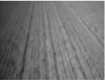
(Barsy, Liroux, Wallay, Acosse). Most of these (29) were encountered in one place (1 out of 16), which may explain a part of the difference between the results of the two years, in Table 2. Figure 6 shows an image extracted from a video acquired at Liroux. The furrow
was clearly visible, but other furrows resulting from the seedbed preparation were visible too. A detailed observation of intermediate results showed that the problem was related with the width of the trace which was very thin compared with the others. In fact the algorithm followed a cluster of less contrasted traces. It was easily possible to ‘tune’ the parameters to solve this problem, but as explained earlier, the parameters fitting was a compromise and tuning the parameters to detect narrower traces would mean to decrease the detection of wide traces. These failures occurred when the sun was approximately overhead, resulting in limited or no shadows (as for Liroux). This was a limitation of the method. This was however not systematic: at other places with similar lighting conditions, other factors such as the moisture of the soil were able to reveal the trace, while some seedbed preparations produced lures (Fig. 6) which could be avoided.
The comparison of the different methods or combinations showed that the Kalman filter applied alone after the Hough transform was not suitable and provided no advantage when used in combination with the recursive filter. The non linear recursive filter was found better for filtering the impulsive noise than the Kalman filter. This later is based on several hypotheses, amongst other white noises with Gaussian distributions. Neither of these requirements were fulfilled. Some test with ‘coloured noise’ (noise having a decreasing power spectrum as the frequency increase, meaning that its value at time step k, Eqns 2 and 3, is somehow correlated to its values at time steps k-1, k-2, ... k-n) showed that the autocorrelation of the noises vk and wk varied from one video to the other and we were
constrained to use the white noise hypothesis. Moreover, the variances of the noises also varied from place to place, depending on the contrast of the furrow with the surrounding matter for the measurement noise (vk) or on the behaviour of the driver for the process noise
(wk). These variations in the noises variances also complicated the rejection of the lures
based on the estimated covariance of the estimated position, as did Tillett et al. (2002). When one image out of five was treated, to simulate the behaviour of the algorithm running at 6 images per second, the increase in the image steps did not change significantly the
results, thus allowing the algorithm to be run on-line on a cost effective processor.
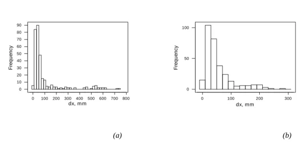
The mean-shift algorithm (with the selection of the absolute maximum) used to retrieve the maxima in the Hough space enhanced significantly the results (Table 2). Particularly, the trueness and the precision of 2003 were strongly reduced. The maximal values were brought from above 700 to below 300, the third quartile were slightly reduced and the median were about the same. Figure 4 shows the frequency distributions of the deviation for the base method and for mean-shift variant. The mode is at the same place as for both methods but the outliers are strongly reduced with the mean-shift variant. With this method, only 9 videos (out of 326, i.e. 3%) presented a deviation above 200 mm and all the concerned videos were acquired at the same place (Liroux).
3.1.3. Comparison with the profile and regression based method
The profile and regression based method showed a trueness and the precision lower than for the Hough transform based method dispersion (higher values of the mean, median and standard deviation, Table 2). The values of the trueness were tested with paired t-test and the medians with paired Wilcoxon rank test. The means were not significantly different, but showed a probability to observe the difference if the mean were equal of 0.06, close to the significance level. The median were very highly significantly different. The standard deviations also showed very high significant differences. The major drawback came from a drop in robustness, with 60 videos presenting deviations over 200 mm which was nearly twice as much as for the Hough transform based method. Only a part of the image was integrated for each profile, which means that the ‘noise’ was less attenuated compared with the Hough transform method.
The Hough transform based methods were able to compute just above 7 images per second (the program treating one image out of five was thus able to treat the whole video in real time), while the regression and profile based method could reach 50 images per second. 3.2. Detection of seed rows
Few parameters had to be fitted. The size of the reduced image were of 120 pixels wide and 90 pixels high, conserving the original width to height ratio. The lines to be detected were sometimes quite thin and smaller image size tended to lessen the results. The Gaussian filter size was 11 pixels in height and 3 pixels in width. This asymmetry contributed to reduce the ‘noise’ while preserving the thin vertical lines. The median filter was square and of 5 pixels. A bigger median filter attenuated wider objects in the background image and thus preserving them better in the final image. This was favourable to reveal the seed rows (the ‘target’) but also for other lines resulting from the soil tillage, for example. These other lines appeared often wider on the images and the parameter fitting led to median filter size relatively small for this application and far smaller than for the detection of the furrow.
The results of the pretreatments are shown in Fig. 3. Most of the shadows were removed by the background subtraction. The contrast which, on the original image, was less important in the shaded part, remained smaller in those parts of the pretreated image. Nevertheless, the lines were visible in that part too. A thin part of the tractor door remained. This linear element has similarities with the seed rows except for its orientation. As the adapted Hough transform was carried out in an interval of 0.3 radians on each side of the vertical in the image, such objects are not considered by the adapted Hough transform and was for this reason not confused with the seed rows. This means that the presence of vertically elongated objects, which may provide shadows with an orientation and a width similar to the seed rows, if these objects are found near the camera, have thus to be avoided to prevent confusions.
The images in the rows 5 in Figs 3, representing the result of the classical Hough plane for angles varying from - π /2 up to π/2 rad, are given for didactic purposes and were not used by the proposed algorithm. The images of the row 6 (Fig. 3) were the results of the adapted Hough transform (for angles varying from -0.3 to 0.3 radian around the reference). For both the classical and the adapted Hough space, the grey scale was scaled so that the
black level represents the minimum and the white level represents the maximum.
In good conditions when the rows were clearly visible, as in Figs 3a, one maxima was observed for each crop row for the classical Hough transform. The detection of these maxima might have been achieved using for example the mean-shift. When the conditions were less favourable, the maxima decreased while others might appear. This can be seen particularly in Fig. 3-5b where highest maxima corresponded to the furrow between the seed rows. The problem of the association of the pairs or triplets of maxima corresponding to the lines in the cluster would became more intense. On the adapted Hough transform, one main maximum was observed in most conditions.
Considering the filtering of the signal resulting from the image analysis, it should be noted that lateral movements of the drilling machine was more likely than an angular movement. Consequently, the values of both coefficients c were different and fixed at 0.002 for cα and at 0.01 for cr.
Table 3 gives a summary of the statistics described above. The trueness and the precision of the method were found to be satisfactory for the application, the rows being localised with a trueness of a few centimetres and a good precision. The third quartile was barely higher than the mean, thanks to the asymmetry of the frequency distribution of the deviation. The maximal values were well beyond the clearance of the machines.
3.3. Comparison
The precision reached in the detection of the seed row was far better than the best method of furrow detection. The detection of the furrow had to deal with traces of quite different widths while the traces left by the drill were of constant width (even if narrow) which was an advantage for the detection. The computation load of both methods was comparable.
5. Conclusions
techniques.
First, methods for the localisation of a furrow in video sequences were presented and compared. Pre-treatment, consisting mainly in a background subtraction, was introduced to avoid the effects of the shadows and was found effective. An image treatment based on the Hough transform and followed by the localisation of the maxima based on Cheng’s mean shift algorithm and by a recursive filter gave the best accuracy. The treatment of 326 videos, acquired during two sowing seasons, showed a trueness (below 65 mm) and a precision (below 55 mm) compatible with the application. The main limitations came from the geometrical characteristics of the illuminant, when two circumstances were both present, no shadow of the furrow was visible and when the soil was dry at the depth of the furrow.
Second, an adapted Hough transform was applied on grey level images for the detection of seed rows. The adaptation consisted in computing one Hough transform per seed row with for reference the theoretical position and orientation of the considered line. This method showed one maxima in the Hough space while the classical method gave one local maxima for each trace. This maxima presented a good contrast in most conditions. The images had to be pretreated with the same algorithms as the in first method, but the traces being narrower, a slighter median filtering was required. The overall performance of the method, showing a deviation from a reference of few centimetres (below 30 mm) was found totally satisfying.
The cost in terms of equipment or computational power are around the same for both techniques. The precision of the seed row detection was found superior and this method will be implemented to control the prototype which shall be tested during the next sowing season.
6. Acknowledgements
This research was funded by the Walloon Region (Direction Générale de la Technologie et de la Recherche), Belgium, convention FIRST SPIN off, 011/4797.
7. References
Benson E R; Reid J F; Zhang Q (2003). Machine-vision based guidance system for agricultural grain harvester using cut-edge detection. Biosystem Engineering, 86(4), 389-398
Cheng Y (1995). Mean Shift, Mode Seeking, and Clustering. IEEE Transactions on Pattern analysis and Machine Intelligence, 17(8), 790-799
Debain C; Chateau T; Berducat M; Martinet P; Bonton P (2000). A guidance-assistance system for agricultural vehicles. Computers and Electronics in Agriculture, 25, 29-51
Hague T; Marchant J A; Tillett N D (2000). Ground based sensing systems for autonomous agricultural vehicles. Computers and Electronics in Agriculture, 25, 11-18
Jahns, G (2000). Special Issue: navigating agriculture field machinery. Computers and Electronics in Agriculture, 25, 1-194
Kalman R E (1960). A new approach to linear filtering and prediction problems. Journal of Basic Engineering. Transactions of the ASME, D 82, 35-45
Marchant J A (1996). Tracking of row structure in three crops using image analysis. Computers and Electronics in Agriculture, 15, 161-179
Onyango C M; Marchant J A (2001). Physics-based colour image segmentation for scenes containing vegetation and soil. Image and vision computing, 19, 523-538
Pilarski T; Happold M; Pangels H; Ollis M; Fitzpatrick K; Stentz A (2002). The Demeter system for automated harvesting. Autonomous Robots, 13, pp. 9-20
Pla F; Sanchiz J M; Marchant J A; Brivot R (1997). Building perspective models to guide a row crop navigation vehicle. Image and Vision Computing, 15, 465-473
Søgaard; Olsen (2003). Determination of crop rows by image analysis without segmentation. Computers and Electronics in Agriculture, 38, 141-158
Sonka M; Hlavac V; Boyle R (1993). Image Processing, Analysis and Machine Vision. Chapman & Hall. London
Stoll A; Kutzbach H D (2000). Guidance of forage harvester with GPS. Precision Agriculture, 2, 281-291
Tillett N D; Hague T (1999). Computer-vision based hoe guidance for cereals – an initial trial. Journal of Agricultural Engineering Research, 74, 225-236
Tillett N D; Hague T; Miles S J (2002). Inter-row vision guidance for mechanical weed control in sugar beet. Computers and Electronics in Agriculture, 33, 163-177
Table 1
Optimal values of the parameters fitted for each of the method combinations
Parameter/ main method + posttreatment, variantImage scaling Standard deviation of the Gaussian filter, pixels Square median filter width, pixels Parameters of the recursive filter Eqn (5) (c) (s) pixels² Process ‘noise’ covariance (Q) pixels² Measurement ‘noise’ covariance (R) pixels² Hough based + recursive filter 0.15 3 7 0.01 5×10 4 - -Hough based + Kalman filter 0.15 3 9 -- 1.6×10³ 3.6×10⁶ Hough based + recursive filter + Kalman filter 0.15 3 9 0.3 5×10⁴ 1.6×10³ 3.6×10⁶ Hough based +
recursive filter, step 5 0.15 3 7 0.01 5×10
4 - -Hough based + recursive filter, mean shift 0.075 2 9 0.01 1×10⁴ - -Regression based + recursive filter + Kalman filter 0.15 1 9 0.7 5×10⁴ 1.6×10³ 3.6×10⁵
Table 2
The results for the various method combinations, post-treatments and eventual variants are summarised with the trueness (mean of the deviation, the absolute differences between the
reference and detection), the precision (standard deviation of the difference), the median, the third quartile and the maximum of the deviation. All the distances are given in mm
Statistic/ Main method + posttreatment,
variant
Year Trueness(mean)(standard deviation)Precision Median Third quartileMaximum deviation
Hough based + recursive filter 2002 2003 64 106 49 156 51 41 66 88 301 731 Hough based + Kalman filter 2002 2003 74 115 62 164 54 43 75 99 378 753 Hough based + recursive filter + Kalman filter 2002 2003 65 101 55 151 54 41 64 74 353 608 Hough based + recursive filter, step 5 2002 2003 64 108 48 157 54 46 67 97 301 660 Hough based + recursive filter, Mean Shift 2002 2003 65 58 34 54 57 39 76 70 157 284 Regression based + recursive filter + Kalman filter 2002 2003 99 125 112 144 57 55 100 158 509 593
Table 3
Main statistics of the deviation with the reference, concerning the detection of seed rows, summarised with the trueness (mean of the deviation, the absolute differences between the reference and
detection), the precision (standard deviation of the difference), the median, the third quartile and the maximum of the deviation. All the distances are given in mm
Trueness
(mean) (standard Precision deviation)
Median Third quartile Maximum
deviation
Mean 28 22 23 38 112
Standard
a b
c d
e f
g
Fig. 1. Images extracted from the different steps of the Hough transform based method. (a) green channel of a colour image extracted from the numeric video sequence : 320×240 pixels; (b) size reduction 48
×36 pixels; (c) low pass Gaussian filtering; (d) rank median filter returning the background; (e) background subtraction; (f) the ‘Hough space’, with horizontally the the angle of the projection line with the horizontal (α) and vertically the distance along the projection line; (g) the detected
Fig. 2. Graphical representation of the different steps of the Profile and regression based method : (a) image was extracted from a video sequence and divided into four strips, the second one being outlined;
and (b) its profile; in light grey, the raw profile; in grey, the median filtered profile (the ‘background’); in black, the difference; the minima were localised on the upper image (a) by dots
a b 1 2 3 4 5 6 7
Fig. 3. Pretreatments of the seed row images: (1) original images; (2) images after resizing and after the Gaussian filter; (3) background images (after median filter); (4) images after background subtraction; (5) image of the classical Hough transform; (6) image of the modified Hough transform; (7) result of the detection; (a) sample image containing a wide shadow; (b) sample
800 700 600 500 400 300 200 100 0 90 80 70 60 50 40 30 20 10 0 dx, mm F re q u en cy 300 200 100 0 100 50 0 dx, mm F re q u en cy (a) (b)
Fig. 4. Histogram of the mean absolute difference with the reference, obtained with the Hough transform based method (a), with the same method and the mean shift variant (b)
Fig. 5. The position returned, for a video, by the Hough transform method alone (raw data, in light grey) and by the whole algorithm (filtered, in dark grey). The reference is in black
Fig. 6. Image extracted from a video and showing the furrow (the most contrasted trace at the first quarter from the left) and lures produced here by the seed bed preparation