HAL Id: hal-01330139
https://hal.archives-ouvertes.fr/hal-01330139
Preprint submitted on 27 Jun 2016
HAL is a multi-disciplinary open access
archive for the deposit and dissemination of
sci-entific research documents, whether they are
pub-lished or not. The documents may come from
teaching and research institutions in France or
abroad, or from public or private research centers.
L’archive ouverte pluridisciplinaire HAL, est
destinée au dépôt et à la diffusion de documents
scientifiques de niveau recherche, publiés ou non,
émanant des établissements d’enseignement et de
recherche français ou étrangers, des laboratoires
publics ou privés.
Public Domain
superimpositions for disparity map estimation
Jean-Charles Bricola, Michel Bilodeau, Serge Beucher
To cite this version:
Jean-Charles Bricola, Michel Bilodeau, Serge Beucher. Morphological processing of stereoscopic image
superimpositions for disparity map estimation. 2016. �hal-01330139�
superimpositions for disparity map estimation
Jean-Charles Bricola, Michel Bilodeau and Serge BeucherPSL Research University – MINES ParisTech CMM – Centre de Morphologie Math´ematique 35 rue St-Honor´e 77300 Fontainebleau, France
Abstract. This paper deals with the problem of depth map computa-tion from a pair of rectified stereo images and presents a novel solucomputa-tion based on the morphological processing of disparity space volumes. The reader is guided through the four steps composing the proposed method: the segmentation of stereo images, the diffusion of superimposition costs controlled by the segmentation, the resulting generation of a sparse dis-parity map which finally drives the estimation of the dense disdis-parity map. An objective evaluation of the algorithm’s features and qualities is provided and is accompanied by the results obtained on Middlebury’s 2014 stereo database.
Keywords: stereo vision, geodesic distances, 3D watershed, image seg-mentation, sparse disparity measurements, dense estimation
1
Introduction
The problem of computing a depth map from a pair of rectified stereo images is undoubtedly a classic one in computer vision. When a point of the scene projects onto the two image planes, it does so with the same ordinates but with different abscissa. The difference of abscissa corresponds to what is commonly referred to as the disparity and is inversely proportional to the point’s depth being sought for. Finding point correspondences between the left and right views of the stereo pair is relatively easy across non-uniformly textured areas. However, homogeneous regions are the source of matching ambiguities whilst the occlusion phenomenon makes it impossible for some pixels to have a correspondence and thus require their disparity to be estimated according to a suitable model.
In order to overcome these two difficulties, it is usual to devise algorithms which ensure, on the one hand, that disparities evolve smoothly across the low-textured areas of the image for which the depth map is estimated and, on the other hand, that disparities remain consistent with the resulting warping of stereo images. Depth discontinuities must be tolerated though in order to han-dle the presence of different objects in the scene. Image gradients and prior segmentations are, to this end, often used as pertinent cues on natural scenes. Furthermore, occluded areas will never, despite correct disparities, yield a mean-ingful superimposition with the other image of the stereo pair. Bad
superimposi-tions for such areas should therefore not prevent the algorithm from giving them the right disparities.
Methods able to satisfy the aforementioned specifications typically belong to the category of global approaches. The general idea is to formulate an energy function which, for a given disparity map, equals the sum of superimposition or warping costs plus a regularisation term, penalising non-smooth disparity transi-tions. Finding the disparity map minimising this energy may be achieved using gradient descent algorithms [1] or, in the context of maximum-a-posteriori or MAP inference, using 3D graph-cuts [2], alpha-expansion [3] and belief propa-gation methods [4–6]. The work of [5] is a good example of how the occlusion phenomenon is taken into account within the MAP inference.
Former methods perform a similar kind of optimisation on each horizontal scanlines independently, so as to warp the corresponding image rows together [7]. Given the disparity space image, the warping is obtained by finding a shortest path going through the corresponding array of accumulated costs, which turns out to be nothing else than a particular type of geodesic distance function. Due to the fact that backtracing, the component of dynamic programming responsible for recovering the shortest path, is employed, the concept cannot easily extend to 3D grids. The combination of scanline optimisations along different axes is nevertheless the main constituent of the semi-global matching [8], which still serves as an essential component in state-of-the-art methods such as [9].
In this article, we propose a novel approach to depth map computation, based on the morphological processing of a disparity space volume, characteris-ing the superimpositions of the considered stereo images for different disparities. A disparity space volume, abbreviated as DSV, is in fact a stack of disparity space images, piled according to an increasing order of disparities. We show how geodesic distance functions computed across a DSV may be employed with the watershed transformation controlled by markers [10], so as to obtain a separat-ing hyperplane between the foreground and background voxels belongseparat-ing to the DSV. Furthermore, our method draws on the idea of [7] which is to integrate ground control points in the process. As a matter of fact, an effort has been made to systematically provide a sparse disparity map carrying a reasonable amount of information, while minimising the number of invalid matches. To fulfil that objective, we got inspired by the research of [11] and [12] in order to diffuse costs inside the disparity space volumes while resorting to the image segmentation so as to prevent incoherent cost aggregations.
The paper starts with four sections which sequentially go through each step of the algorithm. Section 2 presents the morphological segmentation in general and shows how images of the stereo pair are initially partitioned. These partitions add a constraint on our diffusion mechanism presented in section 3, resulting in the generation of sparse disparity maps described in section 4. Then, section 5 provides all the details on the dense disparity map estimation based on the 3D watershed transformation. Finally, section 6 is devoted to the evaluation of the proposed methods on the Middlebury 2014 database.
2
Segmentation
This section explains how both images of the stereo pair are segmented. Our seg-mentation scheme produces partitions which are slightly over-segmented across textured regions, which preserve all contrasted objects even when they are thin and which capture most of the remaining objects’ contours. This choice has been made in the view of the constrained cost diffusion process presented in section 3. Section 2.1 recalls the fundamentals of the watershed transformation, as it is used here in our segmentation procedure but also in sections 4 and 5. Section 2.2 goes into more details about the segmentation algorithm employed in this approach.
2.1 The watershed transformation controlled by markers
Let S : N2 → N be a discrete elevation surface, mapping every point p of the image domain to its altitude S[p]. We define the accompanying image of lakes as L : N2→ N, mapping every point p to a label L[p]. We impose that a point pbelongs to a lake if and only if L[p] > 0.
The watershed transformation of S, controlled by an initial image of lakes L0, is the result of an iterative process which assigns all pixels {p | L0[p] = 0} to a lake existing in L0. The recurrence relationship between Ltand Lt−1is defined as follows:
1. Let St be the set of points reached at altitude t, i.e. St= {p | S[p] ≤ t} 2. The lakes of Lt−1are propagated in an isotropic fashion to all points p ∈ St
having Lt−1[p] = 0 and belonging to a path leading to any lake of Lt−1. 3. The meeting points of lakes of different labels belong to the watershed. When t reaches the highest altitude of S, say t∗, the iterative process stops and the image of lakes Lt∗ is completely filled. Although the algorithm is presented
for two-dimensional elevation surfaces, it applies equally well to any higher di-mension. The reader may find more details on the watershed transformation as well as computationally efficient algorithms based on hierarchical queues in [10].
2.2 Image partitioning with little over-segmentation
In order for Lt∗ to constitute a relevant image partition, both the topographical
surface S and the markers L0 must be chosen appropriately. It is common to define S as a colour gradient, for instance the supremum of the red, green and blue channels’ gradients, when dealing with images of unknown nature. The most trivial choice for the lake’s initialisation then consists of taking each of the gradient’s minima as a marker with a distinctive label, but this typically leads to a severe image over-segmentation, as shown in Figure 2. This is accounted for by the fact that the gradient is, on natural images, composed of a multitude of minima. Filtering the image or the gradient beforehand helps reducing the amount of minima, but care must be taken not to deform the relevant contours.
We propose to alter each level set of the gradient function by applying a series of closings, which decrease exponentially in strength as the altitude of the elevation surface increases. This is exactly the method proposed by [13] for regularising watersheds by oil flooding. The resulting gradients have less min-ima and their watershed transformation produces therefore less over-segmented partitions as testifies Figure 2. Besides, since the closing has little strength at high altitudes, it has little effect on the corresponding level sets and thus sharp contours are not deformed.
Threshold(0,tc) Threshold(0,tf) Label Label AreaOpen(¾c) AreaOpen(¾f)
Threshold(1,+1) Label AreaOpen(¾c)
Merge + W.T. W.T. g – S L L S Mc Mf Mc Mf PartitionBuild Marker function Mask function + – W.T. L S g Lfinal Merge
Fig. 1.Flowchart of the image segmentation procedure.
The partition frontiers obtained at this stage of the proceedings contains the frontiers of the final partition Lfinal. Figure 1 schematises the full segmentation algorithm. Let us briefly describe the operators involved in this system:
– AreaOpen(σ) is an area opening operator which removes any cell of the par-tition having an area inferior or equal to σ pixels.
– Label is a labelling operator which, given a binary image as input, assigns a unique label to every connected component. Pixels set to 0 in the binary image are set to 0 in the labelled image.
– Mergeis responsible for merging two images of markers while ensuring that each of them receives a unique label in the output image.
– PartitionBuildtakes two images of lakes Lmaskand Lmarkeras input. The out-put Loutis an image of lakes of identical dimensions, defined by the following relation:
Lout[p] = (
Lmask[p] if ∃ p′| Lmask[p′] = Lmask[p] ∧ Lmarker[p′] > 0
– Threshold(t0, t1) denotes the standard threshold operator mapping all pixels of the input image in the range [t0, t1] to 1, the others to 0.
– W.T.is the watershed transformation described in section 2.1.
The algorithm’s input g is nothing else than the altered gradient we have pre-viously described. The system represented in the top flowchart yields two inter-mediate images of lakes, called Mc and Mf. The first is meant to hold lakes splitting on very sharp gradient areas while tolerating thin structures. The sec-ond, on the contrary, is more sensitive to smaller contrast but imposes lakes of a certain area. The contrast and area parameters must therefore be chosen, such that tc> tf and σc< σf. The system in the bottom flowchart simply shows how the thin structures in Mc are appended to the image of lakes of Mf and how this results in the final segmentation.
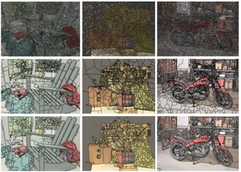
Fig. 2.Sample segmentations for Adirondack, Jadeplant and Motorcycle images from Middlebury 2014 database. The top row shows the result of the watershed transforma-tion of the colour gradient, despite the image pre-filtering, using the gradient’s minima as markers. The middle row is the watershed transformation on the altered gradient g using the gradient’s minima as markers. The bottom row is the output of the algorithm presented in section 2.2.
Regarding the choice of the four parameters, we opted for a solution that is dependant on the image characteristics. tc corresponds to the 45th percentile of the intensity values observed in the initial colour gradient excluding 0, and tf
corresponds to the 10th percentile. Furthermore, it is the ratio of the opening parameter with respect to the full image area which is fixed. In our experiments, this ratio has been set to 5 · 10−5 for σ
c and to ten times more for σf.
3
Costs diffusion
The left and right images of the stereo pair, denoted by I0and I1respectively, are superimposed for different horizontal shifts corresponding to the disparities being tested. The superimpositions are stored in a disparity space volume V : N3→ R. The entry V[x, y, d] reflects how well the pixels of coordinates (x, y) in I0 and (x − d, y) in I1 match. In this approach, V[x, y, d] corresponds to the Hamming distance between the two pixel values in their corresponding Census transformed images [14], encoding the rising edges of the standard gradient according to different directions. This choice makes the superimposition costs insensitive to illumination changes and has become a standard in many stereo applications.
The purpose of costs diffusion is to filter the disparity space volume V so as to highlight the locations where the stereo images effectively superimpose. A trivial choice would be to use a moving average filter which operates on each disparity plane independently, which of course wouldn’t be a good solution. The primary reason is that the moving average filter may obviously aggregate the costs of pixels representing different objects in the scene. This is an issue if the moving average window spans two or more objects with different depths because their costs will be mixed together for the same disparity. In [11], a segmentation of the left image was used to restrict the domain of the aggregation window to the pixels which supposedly belong to the same object as the one of the window centre. In our method, we resort to both the left and right segmentations of the stereo pair, obtained by the algorithm presented in section 2. The domain inside which the diffusion may freely operate, is constrained by the intersection of the left segmentation with the right segmentation shifted according to the considered disparity. This way of proceeding ensures that the costs obtained across the portions of the left image being occluded in the right image do not again mix with the costs obtained across non-occluded areas.
While the chosen segmentations facilitate the construction of quite large ag-gregation supports across homogeneous areas and still consistent ones across thin image structures, the fact that filtering is, at this stage, only applied to each disparity plane independently constitutes a limitation with respect to the processing of tilted and non-planar surfaces. This is why, we shall integrate a basic warping technique to the diffusion scheme.
3.1 Erosions and distance functions
The proposed diffusion algorithm resorts to two morphological operators which, for the sake of completeness, are briefly recalled in this section. Morphological operators are typically controlled by structuring elements which, in the discreet case, are described by sets of points. We will refer to B as an arbitrary structuring element.
Erosions The erosion operator ε under structuring element B transforms a vol-ume V into another volvol-ume εB(V) according to equation 1.
εB(V)[p] = inf
p′∈BV[p + p ′
] (1)
If structuring element B is just composed of one point, such that B = {p′}, the erosion turns into a simple translation in the direction of −p′. In the rest of this article, such a translation will be represented by εp′.
Distance functions The distance function DB(M) associated to a binary volume M: N3 → {0, 1}, and controlled by structuring element B, is expressed by the following recurrence relationship:
Dt= min {Dt−1, εB(Dt−1) + 1} (2)
setting D0[p] = (
0 if M[p] = 0
+∞ otherwise
DB(M) = Dt∗, for t∗ satisfying Dt∗ = Dt∗+1. In fact, DB(M)[p] corresponds to the minimum number of erosions being necessary for voxel p to get reached by any deactivated voxel of mask M, using structuring element B.
3.2 Diffusion algorithm
Let Vs: N3 → N be the volume encoding the intersections of L(0) and L(1), i.e. the partitions of I0 and I1 respectively, for different disparities. Each entry of Vs is computed as:
Vs[x, y, d] = L(0)[x, y] + L(1)[x − d, y] · max x,y L
(0)[x, y] (3)
Suppose that the costs were propagated along a particular direction −t, such that the disparity space volume V would transform into 1
2(V + εt(V)). The set {p | Vs[p] 6= εt(Vs)[p]} determines all the voxels for which costs from different regions would have been mixed. Let Mt stand for the binary mask attributing the value 0 to such voxels and the value 1 to the others. Furthermore, consider the following directions: tl = (−1, 0, 0), tr = (+1, 0, 0), tu = (0, −1, 0) and td= (0, +1, 0).
Algorithm 1 describes the proposed diffusion mechanism. Similarly to [12], the costs are first diffused along the horizontal axis, providing a new filtered disparity space volume, of which the costs in turn are diffused along the vertical axis. However, for each voxel, the aggregation of costs stops as soon as a frontier between two different regions in Vs is crossed or when the maximum diffusion’s scope n has been attained along a particular direction. This is what is enforced by lines 6 and 7 in algorithm 1. As a result, the aggregations along two opposite directions do not necessarily have the same weight and thus more importance is given to the direction where a region border is the farthest away from the considered voxel.
The way algorithm 1 is presented suggests that the diffusion is still con-tained inside each disparity plane. The extension to multiple disparity planes is however quite straightforward and does not change the proposed template. For a given direction t = (tx, ty,0)⊺, we define a new structuring element Bt = {(tx, ty,+1)⊺,(tx, ty,−1)⊺}. The cost update rule in line 5 transforms into:
VUPD← V + min {εt(VOUT), εBt(VOUT) + ξ}
where the parameter ξ controls the regularity of the diffusion. To put it in a nutshell, it is a partial scanline optimisation which is performed along the chosen direction using the left and right image segmentations as a boundary constraint.
Algorithm 1Diffusion of superimposition costs
1: function DirectionalDiffusion(V, t, n) 2: t ←0
3: VOUT← V
4: while t < n do
5: VUPD← V+ εt(VOUT)
6: VSEL←Binary volume highlighting Dt(Mt) > t
7: VOUT← VUPD· VSEL+ VOUT·(1 − VSEL)
8: t ← t+ 1 9: end while 10: return VOUT 11: end function 12: function DiffuseCosts(V, Vs, n) 13: VXL← DirectionalDiffusion(V, tl, n) 14: VXR← DirectionalDiffusion(V, tr, n) 15: VX←(VXL+ VXR) ÷ (min(n, Dtl(Mtl)) + min(n, Dtr(Mtr)) + 2) 16: VYU← DirectionalDiffusion(VX, tu, n) 17: VYD← DirectionalDiffusion(VX, td, n) 18: VY←(VYU+ VYD) ÷ (min(n, Dtu(Mtu)) + min(n, Dtd(Mtd)) + 2) 19: return VY 20: end function
4
Sparse disparity map generation
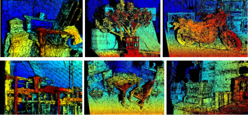
The initial disparity measures are recovered from the filtered disparity space volume computed in section 3, by calculating the disparity that minimises the superimposition cost at each pixel. In addition, cross-checking [15] is performed to ensure that the disparity measures remain consistent between the left and the right images of the stereo pair. The disparity measures which do not satisfy this criterion are discarded. Figure 3 shows some of the resulting disparity maps on the Middlebury 2014 dataset.
Fig. 3.Sparse disparity maps obtained by the diffusion algorithm presented in section 3.2. n is set to 25 pixels. ξ is set to 20% of the maximum possible cost in the disparity space volume V. Pixels appearing in black are those which did not satisfy the cross-checking criterion [15]. Top row shows the disparity maps obtained for Adirondack, Jadeplant, and Motorcycle stereo images. Bottom row shows the disparity maps ob-tained for Pipes, PlaytableP, and Vintage stereo images.
4.1 Detection and pruning of bad measures
Despite their perceptual appeal, these initial disparity maps are subject to some artefacts. It is preferable to detect and remove them if sparse disparity maps were to be used as initialisers of the dense estimation algorithm. Firstly, we observe that artefacts are not predominant in the initial disparity maps. This means that clusters of smoothly evolving disparities should be preserved if they span a significant area of the image. At the opposite extreme, peaky measure-ments should be eliminated without further consideration. The cases in-between demand some more investigation.
Clusters computation In order to find the clusters of smoothly evolving dis-parities, the holes of the initial disparity map are filled in using the watershed transformation presented in section 2.1. The available disparities play the role of initial markers, and the image gradient plays the one of the topographical sur-face controlling the flooding. The gradient of the filled disparity map indicates where disparities do not smoothly evolve. We threshold this gradient between the values 0 and 1 so as to highlight the connected components which uniquely iden-tify the desired clusters. After the labelling, each pixel attributed to a disparity measure receives the identifier of the cluster it belongs to.
Clusters selection The selection of clusters is primarily achieved by the area opening operator introduced in section 2.2. According to the aforementioned specifications, two area openings are performed. The strongest one keeps the
largest clusters while the weakest one removes small impurities. Structures con-served by the weak area opening but removed by the stronger area opening typically correspond to thin image structures or erroneous measures. To tell them apart, it suffices the look at the image gradient and observe that erroneous measures mainly occur across homogeneous areas.
Occlusion artefact filtering Another source of error originates from the diffusion of contour disparities to regions being both homogeneous and textureless. This may be observed, for instance, on Jadeplant (Figure 3) between the top of the elongated box and the background. Since the disparity measures are virtually the same from either side of the frontier, the sole selection of clusters does not suffice to prune the wrong measures, in that scenario. These wrong measures constitute fattening artefacts. In order to detect and remove them, it is important to notice that fattened disparity measures lie near region borders, and are usually not consistent with the disparities found within the interior of the regions. Therefore, we propose to perform the filtering of the fattening artefacts at a regional scale, as follows: each cell of the partition corresponding to the image for which we aim at computing its disparity map, is eroded using an isotropic structuring element of size equal to the diffusion’s scope. The processing then concerns the cells of the partition, which have not been completely destroyed by the erosion. For each of these cells, only the pixels belonging to the cluster(s) covering some area of the corresponding eroded cell, may be restored with their disparity measures. Since the fattened disparities and the interior disparities should belong to different clusters, and that the pixels attributed to the fattened disparities should not belong to the eroded cells, then fattened disparities should not be reconstructed, as desired.
5
Dense disparity map estimation
We aim at estimating the final disparity map by means of a 3D watershed trans-formation. Similarly to any watershed transformation (cf. section 2.1), the suc-cess of the procedure depends on the definition of the initial markers L0: N3→ N and the topographical surface being flooded, S : N3 → N. Since the disparity map is in fact a representation of the hyperplane separating the disparity space volume into the foreground and background voxels, only two markers designat-ing the foreground and background regions are required. Therefore, the markers are initialised so that L0[x, y, d] is equal to the background label ℓg >0 if d = 0, to a distinct foreground label ℓf >0 if d equals the maximum disparity consid-ered with respect to V, and to 0 elsewhere. The most demanding part of this 3D segmentation will be the definition of the topographical surface S.
5.1 Interpolation and distance functions
The topographical volume S should be chosen so that the watershed passes by the points {(xi, yi, di)} for any valid pixel (xi, yi) attributed to disparity di in
(a) (b) (c)
(d) (e) (f)
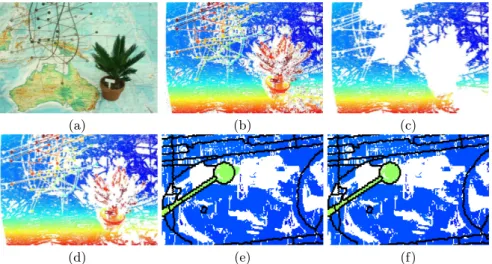
Fig. 4.Illustration of the filtering stage. (a) Left view of AustraliaP, (b) An initial disparity map containing many artefacts, (c) The large clusters of continuous dispari-ties, (d) The union of both large clusters and smaller clusters spanning areas holding sufficient gradient information, (e) Close-up showing the occasional fattening effect on homogeneous areas, (f) Result of the occlusion artefact filtering deduced from the segmentation of the left view.
the filtered sparse disparity map described in section 4. One way of proceeding is to resort to the binary distance function defined by equation 2. In that case, the accompanying mask of control points has to be exclusively set to 0 for all the chosen {(xi, yi, di)} and B must correspond to an isotropic structuring element. In order to drive the watershed transformation, S must therefore equal the in-verted distance function. However, the binary distance function has one major drawback: the fact that the disparity space volume computed in section 3 would be totally ignored from the interpolation process. To overcome this limitation, the geodesic distance controlled by the DSV V may be used instead. The latter is described by equation 4.
Dt= min {Dt−1, εB(Dt−1) + V} (4)
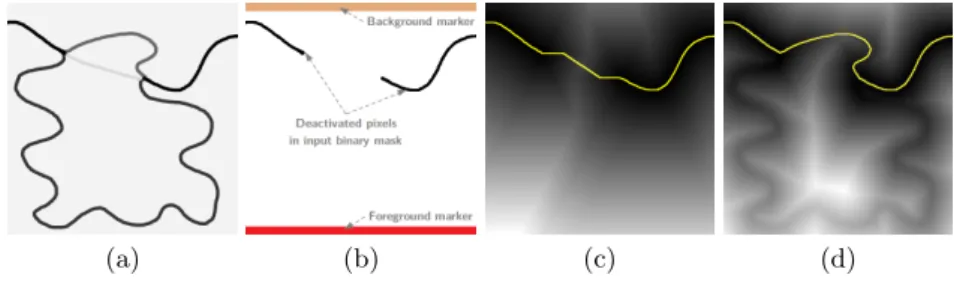
In fact, this equation is a simple alteration of the binary distance update rule (cf. equation 2), where V acts as a viscosity function, delaying the time it takes for a voxel to get reached by one of its neighbours. Figure 5 illustrates the comparison between the segmentations controlled by the additive inverses of the binary and the geodesic distance functions.
5.2 Generation of the topographical volume S
Now, let us explain what the generation of the topographical volume S consists of. At our disposal, we have the segmentation of the left view L(0), the disparity
(a) (b) (c) (d)
Fig. 5.Distance functions and segmentation. (a) Viscosity function, (b) The experi-ment’s settings: in black are shown the pixels from which the distance functions are computed. The coloured rows represent the markers controlling the watershed segmen-tation in conjunction with the inverted distance functions. (c) Binary distance function and resulting watershed shown in yellow. (d) Geodesic distance function controlled by the viscosity functions and resulting watershed segmentation.
space volume V with the aggregated superimposition costs, and a filtered sparse disparity map D. Let D be a distance function, having the same dimensions as V. D is initialised as follows:
D0[x, y, d] = (
0 if D[x, y] = d ∨ k∇L(0)k[x, y] > 0 +∞ otherwise
The points set to zero in this distance function are composed of the control points originating from the sparse disparity map plus the segmentation boundaries of L(0) added to every disparity plane. These boundaries not only guarantee that the interpolation is applied independently on each cell of the partition but also that the hyperplane will fold appropriately at such locations, so as to allow discontinuities within the resulting disparity map.
Once initialised, the computation of the distance function is accomplished using the update rule provided by equation 4. There is one alteration though: similarly to the cost diffusion of section 3, we enforce some regularity by adding a supplementary contribution ζ when accumulating distances across different dis-parity planes. In order to do that, B has to be decomposed into two structuring elements B1and B2, the first holding the directions fronto-parallel to the image plane, the second holding the tilted directions. The term εB(Dt−1) in equation 4 is then replaced by min{εB1(Dt−1), εB2(Dt−1) + ζ}.
Upon convergence at t = t∗
, the topographical volume is finally given by equation 5.
S = −Dt∗+ max
(x,y,d)Dt∗[x, y, d] (5)
6
Experiments and Results
Our method has been tested on the Middlebury 2014 dataset [16], using the quarter resolution images. Both our sparse and dense results are compared to
the ground truth disparity maps acquired using the method described in [17]. This section provides the reader with the parameters chosen to produce all the disparity maps. Then the quality of the sparse disparity measures is evaluated, while discussing the impact of the filtering stage described in section 4. Finally, we analyse the results obtained on the dense disparity maps.
6.1 Parameters
The choices of the segmentation’s parameters are given and explained in section 2. In section 3, two parameters were introduced. ξ, the extra contribution added to the costs aggregated from different disparity planes, is set to 20% of the worst superimposition cost while n, the maximal scope of the diffusion along a particular direction, is fixed to 25 pixels. It should be noted that reducing n is likely to cause the disparity map to become sparser and to be subject to more measurement errors. In section 4, large disparity clusters are supposed to cover at least 0.5% of the image plane against 0.005% for the small clusters. Finally, the regularisation term ζ presented in section 5 is fixed to 50% of the worst superimposition cost.
6.2 Sparse disparity measures
Adirondack ArtL Jadeplant Motorcycle MotorcycleE Piano PianoL Pipes Playroom Playtable PlaytableP Recycle Shelves Teddy Vintage 0.000 0.100 0.200 0.300 0.400 0.500 0.600 0.700
Additional bad pixels (before filtering) Bad Pixels Additional valid pixels (before filtering) Valid Pixels Im a g e o c c u p a n c y r a ti o
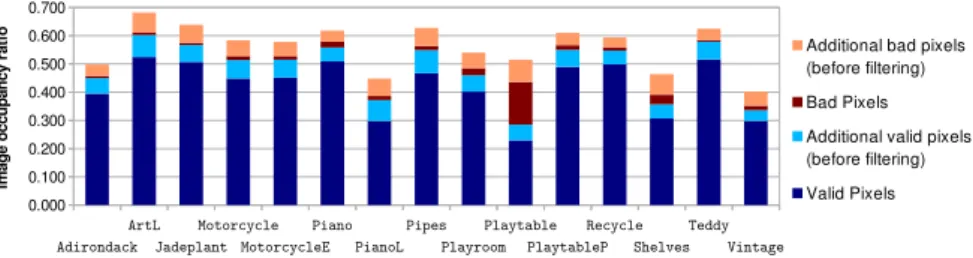
Fig. 6.Occupancy of valid and “bad” disparity measures for the training set of Mid-dlebury 2014 database, before and after the filtering stage.
Some of the initial sparse disparity maps have been presented in Figure 3. Based on the ground truth provided for the training set of the database, the statistics regarding the density and the accuracy of these disparity maps as well as the impact of the post filtering have been gathered in Figure 6. On average, 54% of the pixels covering the non-occluded areas of the image plane have been attributed to a disparity measure. If we consider that erroneous measures are those having a disparity error higher than 2 pixels, then the initial measures have an average error percentage of 12.4%. The filtering stage reduces the latter to 2.80%, while it preserves about 88% of the initial disparity measures which
were correct. Note that the Playtable instance has been discarded from these averages, since the matching errors are the result of severe vertical disparities between the left and right images. The visual appeal of the disparity maps is probably best explained by the fact that they remain consistent with respect to the segmentations computed in section 2, that the absence of measures is recurrent across occluded areas, and that the disparities of pixels being classified as erroneous are still not too different from the ground truth. The root-mean-square error reflects this perfectly well on the benchmark: considering the full image plane, including occluded areas, this error evaluates to 2.2 pixels (quarter resolution), which, at the time of writing, ranks our sparse disparity maps third among those obtained using the other methods evaluated in the benchmark.
Adirondack Jadeplant Motorcycle
Pipes PlaytableP Vintage
AustraliaP Bicycle2 Classroom
Djembe Newkuba Livingroom
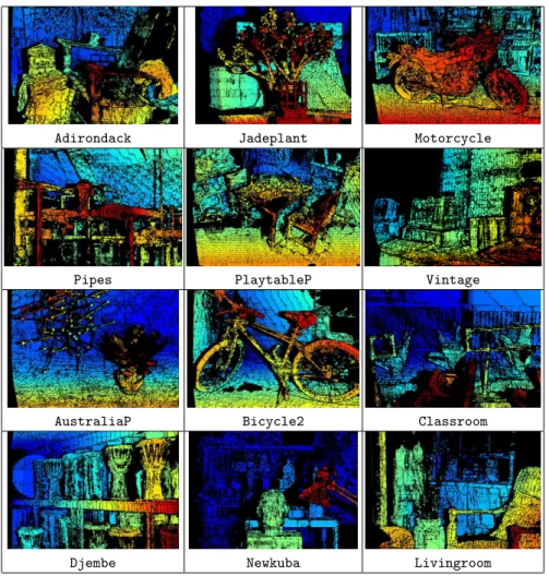
Fig. 7.Sparse disparity maps resulting from the diffusion algorithm, combined with the filtering step presented in section 4.
6.3 Dense disparity map estimation
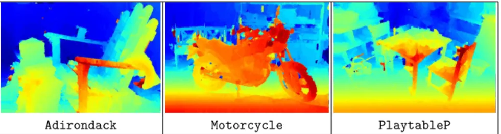
Disparity maps resulting from the interpolation process (cf. section 5) are shown in Figure 8. As desired, the disparity maps are consistent with the provided segmentations, which is again reflected by the RMS error. However, disparities are still subject to inaccuracies across homogeneous areas and the interpolated disparity functions lack of smoothness. As part of a future work, it would in-teresting to study the effect of the viscous watershed transformation [13] on the topographical surface controlling the 3D watershed, since it exhibits interest-ing regularisation properties. Furthermore, the costs obtained across occluded areas should deserve a complementary treatment so that they do not perturb the interpolation when decreasing the regularisation parameter ζ. Finally, the interpolation process could benefit from disparity plane hypotheses, similarly to [18], which could be made on a regional basis, thanks to the sparse disparity measures.
Adirondack Motorcycle PlaytableP
Fig. 8.Disparity maps obtained using the interpolation algorithm presented in section 5, controlled by the corresponding sparse disparity maps.
7
Conclusion
In this study, we have investigated the use of morphological operators within the analysis of stereo image superimpositions and deduced the corresponding disparity maps. The watershed transformation plays a pivotal role in that re-spect, since it is employed for the segmentation of the two images of the stereo pair, the clustering of disparity measures required by the filtering stage, and the interpolation mechanism leading to the dense disparity maps. An important aspect of this work has been the use of the left and right segmentations, in order to avoid irrelevant cost aggregations, perform the pruning of fattening artefacts appearing in the initial sparse disparity maps, and constrain the computation of distance functions used within the interpolation of the final disparity maps. The proposed method yields very good results for the sparse disparity map genera-tion. The dense estimation is the first of its kind to resort to a 3D watershed. While the results are quite encouraging, future work should concentrate on the regularisation of the interpolation process.
References
1. Aydin, T., Akgul, Y.S.: Stereo depth estimation using synchronous optimization with segment based regularization. Pattern Recognition Letters 31(15) (2010) 2389–2396
2. Prince, S.: Models for grids. In: Computer vision: models, learning, and inference. Cambridge University Press (2012)
3. Boykov, Y., Veksler, O., Zabih, R.: Fast approximate energy minimization via graph cuts. IEEE Transactions on Pattern Analysis and Machine Intelligence 23(11) (2001) 1222–1239
4. Sun, J., Li, Y., Kang, S.B., Shum, H.Y.: Symmetric stereo matching for occlusion handling. In: IEEE Computer Society Conference on Computer Vision and Pattern Recognition, 2005. CVPR 2005. Volume 2., IEEE (2005) 399–406
5. Yang, Q., Wang, L., Yang, R., Stew´enius, H., Nist´er, D.: Stereo matching with color-weighted correlation, hierarchical belief propagation, and occlusion handling. IEEE Transactions on Pattern Analysis and Machine Intelligence 31(3) (2009) 6. Facciolo, G., de Franchis, C., Meinhardt, E.: Mgm: A significantly more global
matching for stereovision. In: Proceedings of the British Machine Vision Conference (BMVC), BMVA Press (2015) 90.1–90.12
7. Bobick, A.F., Intille, S.S.: Large occlusion stereo. International Journal of Com-puter Vision 33(3) (1999) 181–200
8. Hirschm¨uller, H.: Stereo processing by semiglobal matching and mutual informa-tion. IEEE Transactions on Pattern Analysis and Machine Intelligence (2008) 9. Zbontar, J., LeCun, Y.: Stereo matching by training a convolutional neural network
to compare image patches. arXiv preprint 1510.05970 (2015)
10. Beucher, S., Meyer, F.: The morphological approach to segmentation: the water-shed transformation. Optical Engineering 34 (1992) 433–481
11. Hosni, A., Bleyer, M., Gelautz, M.: Near real-time stereo with adaptive support weight approaches. In: International Symposium on 3D Data Processing, Visual-ization and Transmission (3DPVT). (2010) 1–8
12. Cigla, C., Alatan, A.A.: Information permeability for stereo matching. Signal Processing: Image Communication 28(9) (2013) 1072–1088
13. Vachier, C., Meyer, F.: The viscous watershed transform. Journal of Mathematical Imaging and Vision 22(2-3) (2005) 251–267
14. Zabih, R., Woodfill, J.: Non-parametric local transforms for computing visual correspondence. In: Third European Conference on Computer Vision 1994 Pro-ceedings, Volume II. Springer Berlin Heidelberg (1994) 151–158
15. Fua, P.: A parallel stereo algorithm that produces dense depth maps and preserves image features. Machine vision and applications 6(1) (1993) 35–49
16. : Middlebury stereo database. http://vision.middlebury.edu/stereo/
17. Scharstein, D., Hirschm¨uller, H., Kitajima, Y., Krathwohl, G., Neˇsi´c, N., Wang, X., Westling, P.: High-resolution stereo datasets with subpixel-accurate ground truth. In: Pattern Recognition. Springer (2014) 31–42
18. Sinha, S.N., Scharstein, D., Szeliski, R.: Efficient high-resolution stereo matching using local plane sweeps. In: IEEE Conference on Computer Vision and Pattern Recognition (CVPR), IEEE (2014) 1582–1589