HAL Id: hal-02266517
https://hal.inria.fr/hal-02266517
Submitted on 14 Aug 2019
HAL is a multi-disciplinary open access
archive for the deposit and dissemination of
sci-entific research documents, whether they are
pub-lished or not. The documents may come from
teaching and research institutions in France or
abroad, or from public or private research centers.
L’archive ouverte pluridisciplinaire HAL, est
destinée au dépôt et à la diffusion de documents
scientifiques de niveau recherche, publiés ou non,
émanant des établissements d’enseignement et de
recherche français ou étrangers, des laboratoires
publics ou privés.
Ontology-Based RDF Integration of Heterogeneous Data
Maxime Buron, François Goasdoué, Ioana Manolescu, Marie-Laure Mugnier
To cite this version:
Maxime Buron, François Goasdoué, Ioana Manolescu, Marie-Laure Mugnier. Ontology-Based RDF
Integration of Heterogeneous Data. [Technical Report] LIX, Ecole polytechnique; Inria Saclay. 2019.
�hal-02266517�
Ontology-Based RDF Integration of Heterogeneous Data
Maxime Buron
Inria and LIX (UMR 7161, CNRS and Ecole polytechnique), France
maxime.buron@inria.fr
Franc¸ois Goasdou ´e
Univ Rennes, CNRS, IRISA, France
fg@irisa.fr
Ioana Manolescu
Inria and LIX (UMR 7161, CNRS and Ecole polytechnique), France
ioana.manolescu@inria.fr
Marie-Laure Mugnier
Univ. Montpellier, LIRMM, Inria Sophia, France
mugnier@lirmm.fr
ABSTRACT
The proliferation of heterogeneous data sources in many ap-plication contexts brings an urgent need for expressive and efficient data integration mechanisms. There are strong ad-vantages to using RDF graphs as the integration format: being schemaless, they allow for flexible integration of data from all sources; RDF graphs can be interpreted with the help of an ontology, describing application semantics; last but not least, RDF enables joint querying of the data and the ontology.
To address this need, we introduce the novel class of RDF Integration Systems (RIS), going beyond the state of the art in the expressive power, that is, in the ability to expose, in-tegrate and flexibly query data from heterogeneous sources through GLAV (global-local-as-view) mappings. Our sec-ond contribution is a set of query answering strategies, two combining existing techniques and three others based on an innovative integration of view-based rewriting; our experi-ments show that the latter bring strong performance advan-tages.
1.
INTRODUCTION
The proliferation of digital data sources across all applica-tion domains brings a new urgency to the need for tools which allow to query heterogeneous data (relational, JSON, key-values, graphs etc.) in a flexible fashion. Since the early days of data integration [26], graphs have been cho-sen as an integration data model, for their flexibility; more recently, the advent of Semantic Web technologies has put forward the RDF data model [1] endowed with the standard SPARQL query language. Beyond its flexibility, RDF brings two qualitative advantages. (i) It is natively connected with standardized ontology languages such as RDFS and OWL; an ontology allows to capture important application knowl-edge, thus querying an integration system through the on-tology allow interpreting the data through the application’s semantic lens; (ii) going beyond logical integration settings based on Description Logics (DL, in short), e.g., [36, 29, 31, 3, 40, 19, 13], SPARQL enables flexible querying of data to-gether with the ontology. For instance, the RDF query “find all the company’s personnel together with their types” is not expressible in a DL setting, just like in SQL, one must spec-ify the relations one wants to query. The ability to query
the data together with the ontology is valuable for complex RDF graphs whose ontology is not fully known to users. For these reasons, in this work we rely on RDF as the inte-gration model, and on ontologies to describe application semantics.
In an integration system, the data sources schemas, com-monly called local schemas, must be related to the integra-tion or global schema [23]. The simplest opintegra-tion is to de-fine each element of the global schema, e.g., each relation (if the global schema is relational), as a view over the local schemas; this is known as Global-As-View, or GAV in short. In a GAV system, a query over the global (virtual) schema is easily transformed into a query over the local schemas, by unfolding each global schema relation, i.e., replacing it with its definition. In contrast, in Local-As-View (LAV) data integration, elements of the local schemas are defined as views over the global one. Query answering in this context requires rewriting the query with the views describing the local sources [32]. GLAV (Global-Local-As-View) data inte-gration generalizes both GAV and LAV. In GLAV scenarios, a query q1over one or several local schemas is associated to
a query over the global schema q2, having the same answer
variables; the pair (q1, q2) is commonly called a mapping.
The semantics is that for each answer of q1, the
integra-tion system exposes the data comprised in an corresponding answer of q2. GLAV maximizes flexibility, or, equivalently,
integration expressive power: unlike LAV, a GLAV mapping may expose only part of a given source’s data, and may combine data from several sources; unlike GAV, a GLAV mapping may include joins or complex expressions over the global schema. Moreover, GLAV mappings enable a certain kind of value invention which (in a precise sense explained in Section 3, Example 9) increases the amount of information accessible through the integration system, e.g., to state the existence of some data whose values are not known in the sources. Thus, in this work, we follow the most ambitious GLAV integration approach.
Ontology-Based Data Access (OBDA) has recently emerged as a data integration paradigm based on the use of ontolo-gies and reasoning [40]. It separates a conceptual level, de-fined by an ontology that describes the application knowl-edge (thus plays the role of the global schema) and a data level defined by data sources, both levels being connected by mappings. Classically, an OBDA system combines a DL
D1, e.g., MongoDB Query q RDFS ontology O Entailment rules R q answers D2, e.g., Jena · · · Dk, e.g., PostgreSQL m1 m2 . . . Mappings M mn Extent E of M based on D1, D2, . . ., Dk RDF integration graph Saturated RDF integration graph
Figure 1: Outline of an RDF Integration System.
ontology, a relational database and GAV mappings (see Sec-tion 6 for details). Our work follows the OBDA vision al-though it implements it in a different setting (RDFS, het-erogeneous data sources and GLAV mappings).
Contributions and novelty The contributions we make in this work are as follows.
(1). RIS Architecture We introduce RDF Integration Systems (RIS, in short), a novel class of integration systems capable of exposing data from heterogeneous sources of vir-tually any data model through GLAV mappings, under the form of an RDF graph endowed with an RDFS ontology; we formalize the problem of BGP (basic graph pattern) RDF query answering on such integration RDF graphs. RIS go beyond the state of the art by applying GLAV mappings to a heterogeneous data setting, and by answering, on the inte-grated RDF graph, queries that are strictly more expressive than allowed in similar systems using DL as the integration model. Thus, RIS provide more flexibility, or, equivalently, the power to express more integration scenarios than previ-ous methods.
To give a global view of our work, Figure 1 outlines a RIS; a full formalization appears in Section 3. Colored areas iden-tify RIS “ingredients”, namely: a set of heterogeneous data sources D1, D2, . . . , Dk; a set of GLAV mappings M; an
RDFS ontology O characterizing the semantics of the inte-gration graph; and a set of inference (or entailment) rules R, which enable reasoning with the ontology. For instance, a rule r ∈ R may state that subclassOf is transitive, i.e., for any semantic classes c1, c2, c3, if c1is a subclass of c2 and c2
is a subclass of c3, then c1 is a subclass of c3; the ontology
may state that a “tempAccountant” is a subclass of “accoun-tant” while the latter is a subclass of “employee”. From D1, . . . , Dk and M derives the extent E, i.e., the source
data exposed by the source queries q1 in the mappings; this
data is transformed into an RDF integration graph. Adding the application ontology O and enriching the result through reasoning with O and rules R leads to more information be-coming available through the RIS, in the saturated RDF in-tegration graph. For instance, if the inin-tegration graph states that Alice is a “tempAccountant”, and assuming O contains the two subclass statements above, its saturation also states that Alice is an “accountant”, and an “employee”. We de-fine RIS query answers with respect to this largest graph, which benefits from the results of ontological reasoning.
(2). Novel, efficient RIS query answering techniques We describe two RIS query answering methods relying on in-gredients known from the previous literature, as well as three novel methods using an innovative transformation of map-pings into materialized views, then relying on view-based rewriting to identify ways to answer the query. We imple-mented all these methods in a platform which combines and extends off-the-shelf components; we provide a quantitative and qualitative analysis of their performance, and identify the last one as the most efficient and robust when the inte-grated data changes.
The paper is organized as follows. Section 2 recalls a set of preliminary notions we build upon. Then, Section 3 defines our RIS and formalizes RIS query answering. Section 4 de-scribes our RIS query answering methods. Section 5 presents our experiments, then we discuss related work and conclude.
2.
PRELIMINARIES
We present the basics of the RDF graph data model (Sec-tion 2.1), of RDF entailment used to make explicit the im-plicit information RDF graphs encode (Section 2.2), as well as how they can be queried using the widely-considered SPARQL Basic Graph Pattern queries (Section 2.3). Then, we recall two reasoning mechanisms on queries (Section 2.4), namely query reformulation and query saturation, as well as the technique of view-based query rewriting (Section 2.5). They will serve as basic building blocks for the query an-swering techniques we shall devise for our RDF integration systems.
2.1
RDF Graph
We consider three pairwise disjoint sets of values: I of IRIs (resource identifiers), L of literals (constants) and B of blank nodes modeling unknown IRIs or literals, a.k.a. la-belled nulls [5, 30]. A (well-formed) triple belongs to (I ∪ B) × I × (L ∪ I ∪ B), and an RDF graph G is a set of (well-formed) triples. A triple (s, p, o) states that its subject s has the property p with the object value o [1]. We denote by Val(G) the set of all values (IRIs, blank nodes and liter-als) occurring in an RDF graph G, and by Bl(G) its set of blank nodes. In triples, we use :b (possibly with indices) to denote blank nodes, and strings between quotes to denote literals.
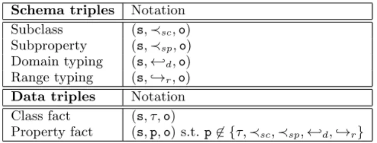
Within an RDF graph, we distinguish data triples from schema ones. The former describe data (either attach a type, or a class, to a resource, or state the value of a cer-tain data property of a resource), while the latter state RDF Schema (RDFS) constraints which relate classes and proper-ties: subclass (specialization relation between types), sub-property (specialization of a binary relation), typing of the domain (first attribute) of a property, respectively, range (typing of the second attribute) of a property. Table 1 intro-duces short notation we adopt for these schema properties. From now on, we denote by Irdf the reserved IRIs from
the RDF standard, e.g., the properties τ , ≺sc, ≺sp, ←-d,
,→r. shown in Table 1. The rest of the IRIs comprises
application-dependent classes and properties, which are said user-defined and denoted byIuser. Hence,Iuser=I \Irdf.
We will consider RDF graphs with RDFS ontologies made of schema triples of the four above flavours. More precisely: Definition 1 (RDFS ontology). An ontology triple is a schema triple whose subject and object are user-defined IRIs fromIuser. An RDFS ontology (or ontology in short)
Schema triples Notation Subclass (s, ≺sc, o)
Subproperty (s, ≺sp, o)
Domain typing (s, ←-d, o)
Range typing (s, ,→r, o)
Data triples Notation Class fact (s, τ, o)
Property fact (s, p, o) s.t. p 6∈ {τ, ≺sc, ≺sp, ←-d, ,→r}
Table 1: RDF triples.
Rule [2] Entailment rule
R rdfs5 (p1, ≺sp, p2), (p2, ≺sp, p3) → (p1, ≺sp, p3) Rc rdfs11 (s, ≺sc, o), (o, ≺sc, o1) → (s, ≺sc, o1)
ext1 (p, ←-d, o), (o, ≺sc, o1) → (p, ←-d, o1)
ext2 (p, ,→r, o), (o, ≺sc, o1) → (p, ,→r, o1)
ext3 (p, ≺sp, p1), (p1, ←-d, o) → (p, ←-d, o) ext4 (p, ≺sp, p1), (p1, ,→r, o) → (p, ,→r, o) rdfs2 (p, ←-d, o), (s1, p, o1) → (s1, τ, o) Ra rdfs3 (p, ,→r, o), (s1, p, o1) → (o1, τ, o) rdfs7 (p1, ≺sp, p2), (s, p1, o) → (s, p2, o) rdfs9 (s, ≺sc, o), (s1, τ, s) → (s1, τ, o)
Table 2: Sample RDFS entailment rules.
is a set of ontology triples. Ontology O is the ontology of an RDF graph G if O is the set of schema triples of G. Above, ontology triples are not allowed over blank nodes. This is only to simplify the presentation; we could have allowed them, and handled them as in [30]. More impor-tantly, we forbid ontology triples from altering the com-mon semantics of RDF itself. For instance, we do not allow (←-d, ≺sp, ,→r), that would impose that the range of every
property shares all the types of the property’s domain! This second restriction can be seen as common-sense; it underlies most ontological formalisms, in particular description log-ics [10] thus the W3C’s Web Ontology Language (OWL), Datalog± [18] and existential rules [38], etc.
Example 1 (Running example, based on [15]). Consider the following RDF graph:
Gex= {(:worksFor, ←-d, :Person), (:worksFor, ,→r, :Org),
(:PubAdmin, ≺sc, :Org), (:Comp, ≺sc, :Org),
(:NatComp, ≺sc, :Comp), (:hiredBy, ≺sp, :worksFor)
(:ceoOf, ≺sp, :worksFor), (:ceoOf, ,→r, :Comp),
(:p1, :ceoOf, :bc), ( :bc, τ, :NatComp),
(:p2, :hiredBy, :a), (:a, τ, :PubAdmin)}
The ontology of Gex, i.e., the first eight schema triples, states
that persons are working for organizations, some of which are public administrations or companies. Further, national companies are particular companies. Being hired by or being CEO of an organization are two ways of working for it; in the latter case, this organization is a company. The facts of Gex, i.e., the four remaining data triples, state that :p1 is
CEO of some company :bc, which is a national company,
and :p2 is hired by the public administration :a.
2.2
RDF Entailment Rules
An entailment rule r has the form body(r) → head(r), where body(r) and head(r) are RDF graphs, respectively called body and head of the rule r. In this work, we con-sider the RDFS entailment rules R shown in Table 2, which are the most frequently used; in the table, all values
except RDF reserved IRIs are blank nodes. For instance, rule rdfs5 reads: whenever in an RDF graph, a property p1 is a subproperty of another property p2, and further p2
is a subproperty of p3 (body of rdfs5), it follows that p1 is
a subproperty of p3 (head of rdfs5). Similarly, rule rdfs7
states that if p1 is a subproperty of p2 and resource s has
the value o for p1, then s also has o as a value for p2. The
triples (p1, ≺sp, p3) and (s, p2, o) in the above examples are
called implicit, i.e., they hold in a graph thanks to the entailment rules, even if they may not be explicitly present in the graph. Following [15], we view R as partitioned in two subsets: the rules Rc lead to implicit schema triples,
while rules Ra lead to implicit data triples.
The direct entailment of an RDF graph G with a set of RDF entailment rules R, denoted by CG,R, is the set of
im-plicit triples resulting from rule applications that use solely the explicit triples of G. For instance, the rule rdfs9 ap-plied to the graph Gex, which comprises ( :bc, τ, :NatComp),
(:NatComp, ≺sc, :Comp), leads to the implicit triple
( :bc, τ, :Comp). This triple belongs to CGex,Ra (hence also
to CGex,R).
The saturation of an RDF graph allows materializing its semantics, by iteratively augmenting it with the triples it entails using entailment rules, until reaching a fixpoint; this process is finite [2]. Formally:
Definition 2 (RDF graph saturation). Let G be an RDF graph and R a set of entailment rules. We recur-sively define a sequence (Gi)i∈N of RDF graphs as follows:
G0= G, and Gi+1= Gi∪ CGi,Rfor i ≥ 0. The saturation
of G w.r.t. R, denoted GR, is Gn for n the smallest integer
such that Gn= Gn+1.
Example 2. The saturation of Gex w.r.t. the set R of
RDFS entailment rules shown in Table 2 is attained after the following two saturation steps:
(Gex)1=Gex∪
{(:NatComp, ≺sc, :Org),
(:hiredBy, ←-d, :Person), (:hiredBy, ,→r, :Org),
(:ceoOf, ←-d, :Person), (:ceoOf, ,→r, :Org),
(:p1, :worksFor, :bc), ( :bc, τ, :Comp),
(:p2, :worksFor, :a), (:a, τ, :Org)}
(Gex)2=(Gex)1 ∪
{(:p1, τ, :Person), (:p2, τ, :Person), ( :bc, τ, :Org)}
2.3
Basic Graph Pattern Queries
A popular RDF query dialect consists of conjunctive queries, also known as basic graph pattern queries, or BGPQs, in short. Let V be a set of variable symbols, disjoint from I ∪ B ∪ L . A basic graph pattern (BGP) is a set of triple patterns (triples in short) belonging to (I ∪ B ∪ V ) × (I ∪ V ) × (I ∪ B ∪ L ∪ V ). For a BGP P , we denote by Var(P) the set of variables occurring in P , by Bl(P ) its set of blank nodes, and by Val(P ) its set of values (IRIs, blank nodes, literals and variables).
Definition 3 (BGP Queries). A BGP query q is of the form q(¯x) ← P , where P is a BGP (also denoted by body(q)), and ¯x ⊆ Var(P) are the answer variables of q. The arity of q is that of ¯x, i.e., |¯x|.
Partially instantiated BGPQs generalize BGPQs and have been used in the literature [30, 15]. Starting from a BGPQ q, partial instantiation replaces some variables and/or blank nodes with values fromI ∪L ∪B, as specified by a substitution σ. The partially instantiated query is de-noted by qσ; we denote by q(¯xσ) its head, and by body(q)σ
its body. Observe that when σ = ∅, qσ coincides with q.
Further, due to σ, and in contrast with standard BGPQs, some answer variables of qσ can be bound:
Example 3. Consider the BGPQ asking for who is work-ing for which kind of company: q(x, y) ← (x, :worksFor, z), (z, τ, y), (y, ≺sc, :Comp), and the substitution σ = {x 7→
:p1}. The corresponding partially instantiated BGPQ qσ is
q(:p1, y) ← (:p1, :worksFor, z), (z, τ, y), (y, ≺sc, :Comp).
The semantics of a (partially instantiated) BGPQ on an RDF graph is defined through homomorphisms from the query body to the queried graph:
Definition 4 (BGP to RDF graph homomorphism). A homomorphism from a BGP q to an RDF graph G is a function ϕ from Val(body(q)) to Val(G) such that for any triple (s, p, o) ∈ body(q), the triple (ϕ(s), ϕ(p), ϕ(o)) is in G, with ϕ the identity on IRIs and literals. Such a homomor-phism is noted G |=ϕq, or simply G |= q to solely denote its
existence.
We distinguish query evaluation, whose result is just based on the explicit triples of the graph, i.e., on BGP to RDF graph homomorphisms, from query answering that also accounts for the implicit graph triples, resulting from en-tailment. Formally:
Definition 5 (Evaluation and answering). Let qσ
be a partially instantiated BGPQ qσ.
The answer set to qσ on an RDF graph G w.r.t. a set R
of RDF entailment rules is: qσ(G, R) = {ϕ(¯xσ) | GR |=ϕ
body(q)σ}. If ¯x = ∅, qσ is a Boolean query, in which case qσ
is false when qσ(G, R) = ∅ and true when qσ(G, R) = {hi},
i.e., the answer to qσ is an empty tuple.
The evaluation of qσ on G, denoted qσ(G, ∅) or qσ(G) in
short, is obtained only through standard BGP-to-RDF ho-momorphisms. It can be seen as a particular case of query answering when R = ∅.
These notions and notations naturally extend to unions of (partially instantiated) BGPQs. For simplicity, below we term UBGPQ a union of BGPQs, whether or not its BG-PQs are partially instantiated.
Example 4. Consider again the BGPQ q from the pre-ceding example. Its evaluation on Gex is empty because Gex
has no explicit :worksFor assertion, while its answer set on Gex w.r.t. R is {h:p1, :NatCompi} because :p1 being CEO
of :bc, :p1 implicitly works for it, and :bc is explicitly a
company of the particular type :NatComp.
We end this section by pointing out that many RDF data management systems use saturation-based query answering, which directly follows the definition of query answering: an RDF graph G is first saturated with the set R of entailment rules, so that the answer set to an incoming query qσ is
obtained through query evaluation as: qσ(GR).
2.4
Reasoning on Queries
Above, we have discussed reasoning on an RDF graph using an ontology, through entailment rules. We now introduce two reasoning techniques which apply on queries.
2.4.1
BGPQ Reformulation
Reformulation-based query answering is an alternative tech-nique to the widely adopted saturation-based query answer-ing. It consists in reformulating a query, so that simple eval-uation of the reformulated query on G yields the complete answer set to the original query on G. Intuitively, reformu-lation injects the ontological knowledge into the query, just
as saturation injects it into the graph. We rely here on the very recent technique of [15], which proposes the first re-formulation algorithm able to take account of the whole set R of entailment rules (recall Table 2). This work extends a previous reformulation algorithm from [30], which is re-stricted to answering queries on data triples, i.e., according to the subset Raof R.
The query reformulation process from [15], which we denote here by Ref(q, O), is decomposed into two steps according to the partition of R into Ra and Rc. The first step, denoted
by Refc(q, O), reformulates a BGPQ q w.r.t. the ontology
O and the set of rules Rc into a UBGPQ, say Qc, which
is guaranteed not to contain ontology triples. Intuitively, this step generates new BGPQs by instantiating variables that query the ontology, e.g., y in a query triple (x, τ, y), with all IRIs (in this case, class IRIs) known in the ontol-ogy. This step is sound and complete w.r.t. Rc, i.e., for
any graph G, q(G, Rc) = Qc(G) = Qc(G \ O) ;
further-more, q(G, R) = Qc(G, Ra). The second step, which we
de-note by Refa(Qc, O), reformulates Qcw.r.t. O and Ra, and
outputs a UBGPQ, say Qc,a. This step is sound and
com-plete w.r.t. Ra, i.e., for any graph G, Qc(G, Ra) = Qc,a(G).
Together, these two steps make reformulation-based BGPQ answering sound and complete [15]:
Theorem 1. For any RDF graph G with O its ontology, and BGPQ q, it holds that q(G, R) = Qc,a(G) = Qc,a(G\O),
where Qc,a= Ref(q, O) = Refa(Refc(q, O), O).
Example 5. The above reformulation of [15] for the query q(x, y) ← (x, :worksFor, z), (z, τ, y), (y, ≺sc, :Comp) from the
preceding example is computed by reformulating first q into Qc= q(x, :NatComp) ← (x, :worksFor, z), (z, τ, :NatComp),
here by instantiating the q’s triple (y, ≺sc, :Comp) on O.
Then, Qcis reformulated into Qc,a=
q(x, :NatComp) ← (x, :worksFor, z), (z, τ, :NatComp) ∪ q(x, :NatComp) ← (x, :hiredby, z), (z, τ, :NatComp) ∪ q(x, :NatComp) ← (x, :ceoOf, z), (z, τ, :NatComp) by specializing :worksFor according to its subproperties in O. It can be checked that Qc,a(Gex) = q(Gex, R) = q(GRex) =
h:p1, :NatCompi, obtained here from the third BGPQ in Qc,a.
2.4.2
BGPQ Saturation
BGPQ saturation has been introduced recently [25] to com-plement a query q with all the implicit triples it asks, given the RDFS ontology O and set R of RDF entailment rules.
Figure 2: BGPQ saturation.
To this aim, the satu-ration of RDF graphs has been extended to BGPs by treat-ing variables as IRIs. Then, the saturation of q w.r.t. R and O, which we note qR,O, is obtained as the saturation of the body of q together with O, using R, from which are pruned out the triples entailed by O but not by body(q), i.e., not relevant to q. The set characterisation of the qR,Otriples is shown in Figure 2; the hatched area corre-sponds to the removed triples. From a practical viewpoint, this characterisation also provides a simple way to compute the saturation of q w.r.t. R and O:
qR,O= (body(q) ∪ O)R\ (OR\ body(q)R)
q(x) ← (x, :hiredBy, y), (y, τ, :NatComp) asking for who has been hired by a national company. Its saturation w.r.t. R, O is: qR,O
(x, y) ← body(q), (x, :worksFor, y), (x, τ, :Person), (y, τ, :Comp), (y, τ, :Org). This saturation is computed as shown above, where the pruned triples are those in OR (be-cause (OR\ body(q)R
) = OR here).
2.5
Query Rewriting-based Data Integration
We recall now the basics of relational view-based query rewrit-ing (Section 2.5.1), which has been extensively studied [32, 23], in particular for the so-called local-as-view data inte-gration. Then we present a generalization of the notion of views as mappings [35] (Section 2.5.2).2.5.1
View-based Data Integration
An integration system I is made of a global schema S (a set of relations) and a set V of views. An instance of S assigns a set of tuples to each relation in S. The data stored in a view V is called its extension. Further, to each view V is associ-ated a query V (¯x) :- ϕ(¯x) over the global schema S, speci-fying how its data fits into S. For instance, let S consist of two relations Emp(eID, name, dID), Dept(dID, cID, coun-try), where eID, dID and cID are respectively identifiers for employees, departments and companies. Consider the views V1(eID, name, dID) :- Emp(eID, name, dID), Dept(dID,
“IBM”, country) providing information about IBM employ-ees, and V2(dID, country) :- Dept(dID, cID, country), which
brings (department, country) pairs. Typically, no single view is expected to bring all information of a given kind; for instance, V1brings some IBM employees, but other views
may bring others, possibly overlapping with V1; this is called
the “Open World Assumption” (OWA).
In an OWA setting, we are interested in certain answers [32], i.e., those that are sure to be part of the query result, know-ing the data present in the views. Such answers can be com-puted by rewriting a query over S, into one over the views V, commonly called view-based rewriting (or rewriting, in short); this can be evaluated over the view extensions in order to produce the answers.
Ideally, a rewriting should be equivalent to the original query, i.e., have the same answers as the query. Such a rewriting may not always exist, depending on the views and the query. For instance, the query q(n, d) :- Emp(e, n, d), Dept(d, c, “France”) does not have an equivalent rewriting using V1
and V2, because only IBM employees are available through
these views. A maximally contained rewriting brings all the query answers that can be obtained through the given set of views; the rewriting may be not be equivalent to q (but just contained in q). In our example, qr(n, d)
:-V1(e, n, d), V2(d,“France”) is a maximally contained
rewrit-ing of q; it returns employees of French IBM departments, whereas the query was not restricted to IBM.
A remarkable result holds for (unions of ) conjunctive queries ((U)CQs), conjunctive views (views V such that the asso-ciated query V (¯x) :- ϕ(¯x) is a CQ) and rewritings that are UCQs: any maximally contained rewriting computes exactly the certain answers. This follows from Theorem 3.2 of [4]; we will build upon this result for answering queries in our RDF integration systems.
2.5.2
Mapping-based Data Integration
The above setting has been generalized to views that are not
necessarily stored as such, but just queries over some under-lying data source. For instance, assuming a data source D holds the relations Person(eID, name) and Contract(eID, dID, salary) with people and their work contracts, the view V1from the above example may be defined on D by: V1D(eID,
name, dID) :- Person(eID, name), Contract(eID, dID, salary) (note that VD
1 hides the salaries from I); V1D provides the
extension of V1. Similarly, view V2may be defined as a query
over some data source (or sources).
Query rewriting is unchanged, whether the views are stored or defined by source queries. In the latter case, to obtain answers, a view-based rewriting needs to be unfolded, re-placing every occurence of a view symbol V with the body of the source query defining that view. Executing the resulting query (potentially over different data sources) computes the answers. This integration setting, which considers views as intermediaries between sources and the integration schema, has been called “global-local-as-view” (GLAV).
An association of a query over a data source and another query over the global schema, e.g., VD
1 and V1above, is
com-monly called a mapping. Depending on the expressiveness allowed for the query over the global schema, a mapping is said either GLAV or just “global-as-view” (GAV). In the for-mer case, the query may comprise non-answer variables thus the view provides an incomplete sub-instance for the global schema, while in the latter case all the variables must be an-swer ones so the view provides a complete sub-instance. For example, suppose that h1,“John Doe”,2i is an answer to V1D
above, hence a tuple in the extension of V1. For this tuple, V1
models in the incomplete sub-instance of S: Emp(1,“John Doe”,2), Dept(2,“IBM”,x), where x is a variable or a labelled null [5] modelling an existing but non-available information. GAV mappings have been used in the ontology-based data access setting to connect data sources to a DL ontology (see Section 6). Here we adopt the more general GLAV mappings to access data from heterogeneous sources through an RDFS ontology; also, we have developed the first concrete system implementing this type of mappings.
3.
PROBLEM STATEMENT
In this section, we first define the notion of RDF integra-tion system (Secintegra-tion 3.1). Then, we state the associated query answering problem (Section 3.2), for which this paper provides solutions in Section 4.
3.1
RDF integration system (RIS)
In an RDF integration system (RIS in short), data from heterogeneous sources, each of which may have its own data model and query language, is integrated into an RDF graph, consisting of: an (RDFS) ontology; and data triples derived from the sources by means of GLAV-style mappings:
Definition 6 (RIS mappings and extensions). A RIS mapping m is of the form m = q1(¯x); q2(¯x) where
q1 and q2 are two queries with the same arity, and further
q2 is a BGPQ whose body contains only triples of the forms:
• (s, p, o) where p ∈Iuser,
• (s, τ, C) where C ∈Iuser.
The body of m is q1 and its head is q2. The extension
of m is the set of tuples ext(m) = {m(δ(v1), . . . , δ(vn)) |
hv1, . . . , vni ∈ q1(D)}, where q1(D) is the answer set of q1
on the data source D and δ is a function that maps source values to RDF values, i.e., IRIs, blank nodes and literals. Intuitively, m specifies that data from D comprised in the
result of query q1, expressed in the native query language
of D, is also present in the RIS integration graph, as result of the (BGP) query q2. Since the actual data resides in
the data sources, m exposes some D data in the integration graph. The extension of m is the set of tuples obtained by instantiating the body of q2 for each result of q1.
Example 7 (Mappings). Consider the two mappings: m1 with head q2(x) ← (x, :ceoOf, y), (y, τ, :NatComp) and
m2 with head q2(x, y) ← (x, :hiredBy, y), (y, τ, :PubAdmin).
Suppose that the body of m1 returns hpD1i as its results,
and that the δ function maps the value pD1
1 from the data
source D1 to the URI :p1. Then, the extension of m1 is:
ext(m1) = {m1(:p1)}. Further, suppose that the body of m2
returns hpD2
2 , a
D2i, and that δ maps the values pD2
2 , a D2 from
the data source D2 to the URIs :p2, :a. Then, the extension
of m2 is: ext(m2) = {m2(:p2, :a)}.
Given a set of RIS mappings M, the extent of M is the union of the mappings’ extensions, i.e., E =S
m∈M ext(m),
and we denote by Val(E) the set of values occurring in E. We can now define the RIS data triples induced by some mappings and an extent thereof.
Definition 7 (RIS data triples). Given a set M of RIS mappings and an extent E of M, the RIS data triples induced by M and E form an RDF graph defined as follows: GME =
[
m=q1(¯x);q2(¯x)∈M
{bgp2rdf(body(q2)[¯x←¯t])) | m(¯t) ∈ E}
where
• body(q2)[¯x←¯t]is the BGP body(q2) in which the answer
variables ¯x are bound to the values in the tuple m(¯t), part of E;
• bgp2rdf(·) is a function that transforms a BGP into an RDF graph, by replacing each variable by a fresh blank node.
The RIS data triples are exactly all the data available to queries through a RIS. Mappings allow to (i) select only the data relevant to a given application, and (ii) organize it according to the shape desired in the integration RDF graph. These triples may, but do not have to, be materialized, as we discussed in Section 4. Observe that by definition, RIS data triples may include some invented values, that is, fresh blank nodes as exemplified below.
Example 8. Reusing the mappings from Example 7, let M = {m1, m2} and its extent E = {m1(:p1), m2(:p2, :a)}.
The RIS data triples they lead to are:
GME = {(:p1, :ceoOf, :bc), ( :bc, τ, :NatComp),
(:p2, :hiredBy, :a), (:a, τ, :PubAdmin)}
Note that GME features some incomplete information: the
first and second triples contain the blank node :bc,
intro-duced by bgp2rdf instead of the variable y in the head (query q2) of m1. Only non-answer variables in a mapping head
lead to blank nodes being introduced in this way in RIS data triples: by Def. 7, answer variables in q2 are replaced with
values from m(¯t) (thus, from Val(E)).
Finally, we define a RIS as a tuple S = hO, R, M, Ei stat-ing that S allows to access (query), with the reasonstat-ing power given by the set R of RDFS entailment rules, the RDF graph comprising the ontology O and the data triples induced by the set of mappings M and their extent E.
3.2
Query answering problem
The problem we consider is answering BGPQs in a RIS. We define certain answers in a RIS setting as:
Definition 8 (Certain answer set). The certain an-swer set of a BGPQ q on a RIS S = hO, R, M, Ei is:
cert(q, S) = {ϕ(¯x) | (O ∪ GME ) R
|=ϕq(¯x)} where ϕ(¯x) comprises only values from Val(E).
cert(q, S) is the subset of q(O ∪ GME , R) restricted to
com-plete answers, i.e., tuples fully built from source values; tu-ples with blank nodes introduced by the bgp2rdf function in Def. 7 are excluded from cert(q, S). Note, however, that the incompleteness (blank nodes) introduced in Def. 7 can be exploited to answer queries, as shown below.
Example 9. Consider the RIS S made of the ontology O of Gexin Example 1, the set R of entailment rules shown in
Table 2, and the set of mappings M together with the extent E from Example 8.
Let q(x, y) ← (x, :worksFor, y), (y, τ, :Comp) be the query asking “who works for which company”, while the query q0(x) ← (x, :worksFor, y), (y, τ, :Comp) asks “who works for some company”. The only difference between them is that y is an answer variable in q and not in q0. The certain answer of q is ∅, while the certain answer of q0 is h:p1i. This
an-swer results from the RIS data triples (:p1, :worksFor, :bc),
( :bc, τ, :Comp), which are entailed from:
• the GM
E triples (:p1, :ceoOf, :bc), ( :bc, τ, :NatComp),
with the blank node :bc discussed in Example 8, and:
• either the O triples (:ceoOf, ≺sp, :worksFor),
(:ceoOf, ,→r, :Comp) together with the R rules rdfs3,
rdfs7, or the O triples (:ceoOf, ≺sp, :worksFor),
(:NatComp, ≺sc, :Comp) together with the R rules
rdfs3, rdfs9.
Because “invented” blank nodes are not allowed in cert(q, S), q has no answer. In contrast, its close variant q0 allows finding out that :p1 is CEO of some national company, even
though the mapping m1 (the only one involving companies)
does not expose the company URI through the RIS. The presence of bgp2rdf-inserted blank nodes may increase the amount of information one can get from a RIS, even if such nodes are not allowed in certain answers. In turn, such blank nodes are enabled by non-answer variables in the heads of the expressive GLAV mappings we consider.
The problem we study in the next Section is:
Problem 1. Given a RIS S, compute the certain answer set of a BGPQ q on S, i.e., cert(q, S).
4.
QUERY ANSWERING IN A RIS
This section is devoted to our core technical contributions: RIS query answering approaches. Def. 8 outlines the tasks involved: (i) computing the RIS data triples GME ; (ii)
rea-soning on this graph, with the ontology O, under the RDFS entailment rules R; (iii) computing answers to the user query q on the graph resulting from the reasoning.
Below, we present five strategies for the RIS query answer-ing problem; they differ in when and how these steps are performed. Specifically, Section 4.1 presents two methods which start by actually computing the RIS data triples; this is reminiscent of an extract-transform-load (or ware-house) scenario in classical data integration literature [39], followed by an RDF query answering stage (as recalled in Section 2.2). The strategies described in Section 4.2 are our most innovative ones; they use the mappings as views, in order to reduce query answering in a RIS to relational view-based query rewriting (recalled in Section 2.5.1).
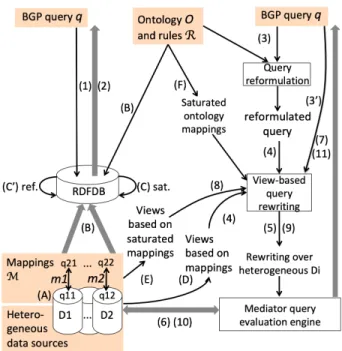
Figure 3: Outline of query answering strategies.
4.1
RIS Query Answering through RIS Data
Materialization:
MATand
MAT-CAWe first present two strategies which materialize the RIS data triples, then reduce RIS query answering to RDF query answering: either based on graph saturation (MAT), or on query reformulation (MAT-CA, whose acronym reflects refor-mulation with both the Rc and Ra rules from Table 2).
Figure 3 traces the various steps involved in our strategies; the thick gray arrows follow data (partial or final query an-swers), whereas the others trace transformations applied on the query, mappings, and/or ontology, all of which are typ-ically orders of magnitude smaller than the data. The main algorithmic building blocks, e.g., “View-based rewriting”, are shown in boxes; the figure also shows some partial com-putation results being exchanged during query answering, e.g., “Saturated mappings” etc. During materialization, the q1 queries part of each mapping are executed (step (A)),
then their results are converted as per Def. 7 into RIS data triples, which are stored into an RDF data management sys-tem (step (B)).
Then, when a BGPQ q is asked (step (1)) against the RDF graph G made of the RIS data triples and the ontology O, it can be answered (step (2)): either by the saturation-based technique (step (C)) on the graph G saturated with the set R of RDFS entailment rules, or by the reformulation-based technique (step (C’)), reformulating q using O and R into a UBGPQ Qc,a (recall Section 2.4.1), then evaluating Qc,a
on the RIS data triples only.
The next theorem states the correctness of our two above-mentioned RIS query answering methods:
Theorem 2 (MATandMAT-CAcorrectness). Let q be a BGPQ asked on the RIS S = hO, R, M, Ei, whose ma-terialized RDF graph is G = O ∪ GME . Then:
• cert(q, S) = {ϕ(¯x) | GR|=ϕ q(¯x), ϕ(¯x) ⊆ Val(E)|¯x|}; • cert(q, S) =Sn i=1{ϕ(σi(¯x)) | G |= ϕqi σi(¯x), ϕ(σi(¯x)) ⊆ Val(E)|¯x|} withSn i=1q i
σi(¯x) the reformulation Qc,a of q
w.r.t. O, R (recall Section 2.4.1).
The proofs of the above items follow from the definition of certain answers in a RIS (Def. 8), and either from that of RDF query answers (Def. 5) for the saturation-based ap-proach (first item) or from Theorem 1 for the reformulation-based approach (second item).
Example 10. Consider the RIS of Example 9, whose on-tology O and GME data triples form exactly the Gex RDF
graph in Example 1. Examples 4 and 5 therefore also il-lustrate how queries are handled within this RIS, through
MATorMAT-CA query answering.
These two methods push the extent materialization work be-fore queries are received, thus speeding up query answering. However, the materialized RIS data triples must be main-tained when the data sources are updated. In turn, changes to the RIS data triples changes require maintaining GRfor the saturation-based strategy. Hence, approaches based on materializing RIS data triples are generally not adapted to contexts where data changes frequently.
4.2
RIS Query Answering through View-based
Query Rewriting
Next, we discuss RIS query answering strategies based on view-based query rewriting. The first (Section 4.2.1) com-bines query reformulation and relational view-based query rewriting; such a combination has been used to in-tegrate data in a centralized [29, 31, 40] or peer-to-peer [3] description logic setting, but, to the best of our knowledge, not in the RDF one. In contrast, the last two (Section 4.2.2) rely on intricate combinations of query reformulation, query saturation (Section 2.4.2) and relational view-based query rewriting. As we will show, BGPQ saturation allows reduc-ing significantly the query-time reasonreduc-ing effort.
For our discussion, we introduce a set of simple functions. The bgp2ca function transforms a BGP into a conjunction of atoms with ternary predicate T (standing for “triple”) as fol-lows: bgp2ca({(s1, p1, o1), . . ., (sn, pn, on)}) = T (s1, p1, o1)∧
· · ·∧T (sn, pn, on). The bgpq2cq function transforms a BGPQ
q(¯x) ← body(q) into a CQ q(¯x) ← bgp2ca(body(q)). Fi-nally, the function ubgpq2cq function transforms a UBGPQ Sn
i=1qi(¯xi) into a UCQ by applying the above bgpq2cq
func-tion to each of its qi.
4.2.1
Rewriting Reformulated Queries using
Map-pings as Views:
REW-CAIn this approach, the incoming BGPQ q is first reformulated (recall Section 2.4.1) into a UBGPQ Qc,a with the ontology
O and rules R; reformulation with Rc and Ra accounts for
the second part of the acronym. However, here, Qc,acannot
be evaluated on the RIS data triples, because they are not materialized. Instead, we view each mapping as a relational LAV view over the integration graph, and rewrite the query based on these views. Specifically, such views are defined on the global relational schema {T }, where T is the triple relation introduced earlier in this section:
Definition 9 (Mappings as relational views). Let m = q1(¯x) ; q2(¯x) be a mapping. Its corresponding
relational view is: m(¯x) ← bgp2ca(body(q2)).
Example 11. The relational views corresponding to the mappings m1, m2 from Example 7 are:
• m1(x) ← T (x, :ceoOf, y), T (y, τ, :NatComp)
• m2(x, y) ← T (x, :hiredBy, y), T (y, τ, :PubAdmin)
Qc,a=
q(x, :ceoOf) ← T (x, :ceoOf, z), T (z, τ, :NatComp), T (x, :worksFor, a), T (a, τ, :PubAdmin) ∪ q(x, :ceoOf) ← T (x, :ceoOf, z), T (z, τ, :NatComp),
T (x, :hiredBy, a), T (a, τ, :PubAdmin) ∪ q(x, :ceoOf) ← T (x, :ceoOf, z), T (z, τ, :NatComp),
T (x, :ceoOf, a), T (a, τ, :PubAdmin) ∪ q(x, :hiredBy) ←T (x, :hiredBy, z), T (z, τ, :NatComp),
T (x, :worksFor, a), T (a, τ, :PubAdmin) ∪ q(x, :hiredBy) ←T (x, :hiredBy, z), T (z, τ, :NatComp),
T (x, :hiredBy, a), T (a, τ, :PubAdmin) ∪ q(x, :hiredBy) ←T (x, :hiredBy, z), T (z, τ, :NatComp),
T (x, :ceoOf, a), T (a, τ, :PubAdmin) Figure 4: Sample reformulation for Example 12.
is denoted by Views(M). Crucially, the extent E of the mapping set M is also an extent for the corresponding set of views Views(M). In particular, we establish that the certain answers to a BGPQ q on a RIS (Def. 8) are exactly the certain answers of its UBGPQ reformulation Qc,a seen
as a UCQ w.r.t. the relational CQ views obtained from the RIS mappings.
Theorem 3 (REW-CA correctness). Let S = hO, R, M, E i be a RIS and q be a BGPQ. Let Qc,a be the reformulation
of q w.r.t. O and R. Then:
cert(q, S) = cert(ubgpq2ucq(Qc,a), Views(M), E)
where cert(ubgpq2ucq(Qc,a), Views(M), E) denotes the
cer-tain answer set of ubgpq2ucq(Qc,a) over Views(M) and E.
This result relies on the soundness and completeness of refor-mulation (Theorem 1), which implies that cert(q, S) is equal to cert(Qc,ah∅, ∅, M, Ei); by construction of ubgpq2ucq(Qc,a)
and Views(M), cert(Qc,ah∅, ∅, M, Ei) is in turn equal to
cert(ubgpq2ucq(Qc,a), Views(M), E) .
The above theorem leads to the following query answering strategy (Figure 3): reformulate q into a UBGPQ Qc,a(step
(3)), translate it into a UCQ, and provide this UCQ as input to a relational view-based query rewriting engine (step (4)), together with the relational views. The view-based rewrit-ing thus obtained (step (5)) refers to the view symbols corre-sponding to the mappings, e.g., m1, m2 etc.Next, we unfold
each such view symbol by replacing it with the body of the query q1 from the respective mapping (recall that q1 is
ex-pressed in the native language of the data source). This yields an expression built with (relational) unions, joins, se-lections and projections, on top of a set of source queries. We turn this to a mediator engine, which: interacts with the sources (6) to request the evaluation of the queries q1
involved in the rewriting, possibly pushing inside them se-lections, projections, joins etc., applies any remaining op-erations, such as joins and unions, within the mediator’s runtime component, and returns the results thus computed, which are the answers to q (7).
Example 12. Consider again the RIS in Example 9 and the query q(x, y) ← (x, y, z), (z, τ, t), (y, ≺sp, :worksFor),
(t, ≺sc, :Comp), (x, :worksFor, a), (a, τ, :PubAdmin) asking
“who works for some public administration, and what re-lationship he/she has with some company”. Its UBGPQ reformulation, obtained with the technique in [15] (recall Section 2.4.1), seen as a UCQ is shown in Figure 4. Its maximally-contained rewriting based on the views obtained
from the RIS mappings, for instance with the Minicon al-gorithm [41], is: q(x, :ceoOf) ← m1(x), m2(x, y). It is
ob-tained from the second CQ in the above union; this becomes clear when the view symbols are replaced by their bodies: q(x, :NatComp) ← T (x, :ceoOf, y1), T (y1, τ, :NatComp),
T (x, :hiredBy, y2), T (y2, τ, :PubAdmin). Note that the five
other CQs cannot be rewritten based on the available views. With the current RIS, this rewriting yields an empty certain answer set to the asked query, i.e., cert(q, S) = ∅, because the extent of the mappings, hence of the views, is: E = {m1(:p1), m2(:p2, :a)}. However, if we add m2(:p1, :a) to
E, then cert(q, S) = {h:p1, :ceoOfi}.
4.2.2
Rewriting Partially-Reformulated Queries
us-ing Saturated Mappus-ings as Views:
REWand
REW-CInstead of pushing reasoning into the query by reformulat-ing it, we can push it into the mappreformulat-ings from which we derive the materialized views. To this aim, we saturate the heads of the RIS mappings so that they directly integrate the heterogeneous data sources w.r.t. both the explicit and implicit knowledge the RIS has, i.e., by taking into account the ontology O and entailment rules R. Specifically:
Definition 10 (Saturated mappings). Given an RDFS ontology O, the saturation of a set M of RIS map-pings w.r.t. O is: Ma,O = [ m∈M {m = q1(¯x); q Ra,O 2 (¯x) | m = q1(¯x); q2(¯x)}.
Recall from Section 2.4.2 that qRa,O
2 denotes the saturation
of q2 with Ra and O; it complements the query with all it
implicitly asks for w.r.t. Raand O.
Example 13. Consider the RIS of Example 9, its satu-rated mapping heads are (added implicit triples are in gray):
m1: qR2a,O(x) ← (x, :ceoOf, y), (y, τ, :NatComp)
(x, :worksFor, y), (y, τ, :Comp) (x, τ :Person), (y, τ, :Org)
m2: qR2a,O(x, y) ←(x, :hiredBy, y), (y, τ, :PubAdmin)
(x, :worksFor, y), (y, τ, :Org) (x, τ, :Person)
To take the saturated ontology into account, we propose two different techniques. The first, calledREW, consists of making the (saturation of ) the ontology accessible through specific mappings, one for each kind of schema triple:
Definition 11 (Ontology mappings). The set of mappings assigned to an ontology O is:
MOc=
[
x∈{≺sc,≺sp,←-d,,→r}
{mx| mx= q1(s, o); q2(s, o)}
with q2(s, o) ← (s, x, o). The extension of a mapping mx is
ext(mx) = {(s, o) | (s, x, o) ∈ ORc}. The extent of MOc is
denoted EOc.
Ontology mappings do not fulfill RIS mapping restrictions, they use RDFS properties in their head. Users can not define such mappings as RIS ingredient, because general mappings may lead to incomplete query answering approaches. For this reason, ontology mappings are used in a specific RIS, and they can be considered as RIS mappings for rest of the process. These mappings can be computed offline, and need to be updated when ontology is updated.
Based on the saturated mappings and the ontology map-pings, as well as their extensions, query answers can be com-puted disregarding the entailment rules R and the ontology
q(x, :ceoOf) ← m1(x), m≺sp(:ceoOf, :worksFor),
m≺sc(:NatComp, :Comp), m2(x, a)
∪ q(x, :ceoOf) ← m1(x), m≺sp(:ceoOf, :worksFor),
m≺sc(:Comp, :Comp), m2(x, a)
∪ q(x, :ceoOf) ← m1(x), m≺sp(:ceoOf, :worksFor),
m≺sc(:Org, :Comp), m2(x, a)
∪ q(x, :worksFor) ←m1(x), m≺sp(:worksFor, :worksFor),
m≺sc(:NatComp, :Comp), m2(x, a)
∪ q(x, :worksFor) ←m1(x), m≺sp(:worksFor, :worksFor),
m≺sc(:Comp, :Comp), m2(x, a)
∪ q(x, :worksFor) ←m1(x), m≺sp(:worksFor, :worksFor),
m≺sc(:Org, :Comp), m2(x, a)
∪ q(x, :hiredBy) ← m2(x, z), m≺sp(:hiredBy, :worksFor),
m≺sc(:PubAdmin, :Comp), m2(x, a)
∪ q(x, :hiredBy) ← m2(x, z), m≺sp(:hiredBy, :worksFor),
m≺sc(:Org, :Comp), m2(x, a)
∪ q(x, :worksFor) ←m2(x, z), m≺sp(:worksFor, :worksFor),
m≺sc(:PubAdmin, :Comp), m2(x, a)
∪ q(x, :worksFor) ←m2(x, z), m≺sp(:worksFor, :worksFor),
m≺sc(:Org, :Comp), m2(x, a) ∪ S r∈{≺sc,≺sp,←-d,,→r}q(x, r) ← mr(x, z), m2(v, z), m≺sp(r, :worksFor), m≺sc(:PubAdmin, :Comp), m2(x, a) ∪ q(x, r) ←mr(x, z), m2(v, z), m≺sp(r, :worksFor), m≺sc(:Org, :Comp), m2(x, a)
Figure 5: Sample rewriting for Example 14.
O at query processing time:
Lemma 1. Let S = hO, R, M, E i be a RIS and q be a BGPQ. Then:
cert(q, S) = cert(q, h∅, ∅, MOc∪ Ma,O, EOc∪ Ei)
The main underpinning for this is that reasoning using R can be split according to Raand Rc[15], which are applied
independently on respectively data triples (using the unsat-urated ontology) and ontology. It follows that the induced graphs of S and h∅, ∅, MOc∪ Ma,O, EOc∪ Ei are the same,
hence the certain query answers in these two RIS as well. Recalling from the start of Section 4 the steps involved in RIS query anwering, the above lemma states how to encap-sulate reasoning with the ontology O and the rules R, into the ontology mappings and their extension. In particular, turning this (larger) set of mappings MOc∪ Ma,Ointo
rela-tional views as in Section 4.2.1, we establish that the certain answers of a BGPQ q on a RIS are exactly the certain an-swers of q seen as a CQ w.r.t. these views:
Theorem 4 (REWcorrectness). Let S = hO, R, M, E i be a RIS and q be a BGPQ. Then:
cert(q, S) = cert(bgpq2cq(q), Views(MOc∪ Ma,O), EOc∪ E)
Example 14 (REW). Consider again the RIS in Ex-ample 9 and the query q of ExEx-ample 12 seen as a CQ:
q(x, y) ←T (x, y, z), T (z, τ, t), T (y, ≺sp, :worksFor),
T (t, ≺sc, :Comp), T (x, :worksFor, a),
T (a, τ, :PubAdmin)
Its maximally-contained rewriting based on the views ob-tained from the RIS saturated and ontology mappings ap-pears in Figure 5.
If we assume that E also contains m2(:p1, :a), as we did
in Example 12, we obtain again cert(q, S) = {h:p1, :ceoOfi},
which results from the evaluation of the first CQ in the above UCQ rewriting; the other CQs yield empty results because some required ≺sc or ≺sp contraints are not found in the
views built from the RIS ontology mappings.
Below, we introduce a last approach for certain query anwer-ing on RIS denotedREW-C. Instead of making the saturated ontology explicit in the mappings, we partially reformulate q using Rc (thus the-Csuffix in its acronym). This
corre-sponds to the first step of the reformulation technique pre-sented in Section 2.4.1. The reformulation w.r.t. Rc leads
to the equality of cert(q, hO, R, M, Ei) and cert(Qc, hO, Ra,
M, Ei). We recall that the Qcreformulation obtained after
this first step does not contain any schema triple anymore: it evaluation only requires data triples. Therefore the satu-rated mappings are sufficient to answer it. These observa-tions lead to variants of the previous lemma and theorem:
Lemma 2. Let S = hO, R, M, E i be a RIS, q be a BGPQ and Qc its reformulation w.r.t. O, Rc [15]. Then:
cert(q, S) = cert(Qc, h∅, ∅, Ma,O, Ei)
Theorem 5 (REW-Ccorrectness). Let S = hO, R, M, Ei be a RIS, q be a BGPQ and Qc its reformulation
w.r.t. O, Rc.Then:
cert(q, S) = cert(bgpq2cq(Qc), Views(Ma,O), E)
Example 15 (REW-C). Consider again the RIS in Ex-ample 9 and the query q of ExEx-ample 12. Its Qcreformulation
w.r.t. O, Rc, seen as a UCQ, is:
q(x, :ceoOf) ← T (x, :ceoOf, z), T (z, τ, :NatComp), T (x, :worksFor, a), T (a, τ, :PubAdmin) ∪ q(x, :hiredBy) ←T (x, :hiredBy, z), T (z, τ, :NatComp),
T (x, :worksFor, a), T (a, τ, :PubAdmin) This reformulation is therefore rewritten using the RIS views as: q(x, :ceoOf) ← m1(x), m2(x, a). It is obtained from the
first CQ in the above; the second one has no rewriting based on the available RIS views. We obtain a rewriting isomor-phic to the one obtained in Example 12, hence the same answers as by the above approaches.
In Fig. 3,REW andREW-C are pictured as follows. Offline (independent of the arrival of a query), relational CQ views are computed from the saturated source-to-RIS mappings (step (E)). In REW, these views are complemented with a special set of views derived from O and the ontological map-pings (step (F)). Then, every incoming BGPQ q (step (3’)) is transformed into a CQ and rewritten into a UCQ using the views (step (8)). In contrast,REW-C does not consider on-tological mappings; reasoning with O takes place at query time, by reformulating q into a BGPQ Qc (variant of (3)
considering only Rc), which is then transformed into a UCQ
(variant of (4)) and rewritten still as a UCQ (variant of (8)) using the set of views obtained through step (E). Once a rewriting is obtained, its optimization and evaluation is del-egated to the mediator (steps (9) and (10)), leading to the obtention of query answers (step (11)).
How do our strategies differ? Importantly, since all strategies based on view-based rewriting are correct, they lead to equivalent UCQ rewritings as soon as the same set of
mappings is considered. This means thatREW-CAand REW-C yield equivalent rewritings. StrategyREW considers the additional set MOc of ontology mappings. Hence, theREW
rewriting is larger than the one obtained by REW-CA and
REW-Cfor queries over the ontology (i.e., when q contains triples with ≺sc, ≺sp, ←-d, ,→r or a variable in property
position); otherwise, MOc is not used for query rewriting,
and the three strategies yield equivalent results. Rewritings may contain redundancies, which we remove by minimiza-tion. It is well-known that equivalent UCQs are isomorphic (i.e., equal up to variable renaming) once minimized. Hence,
REW-CAandREW-Cdiffer in how the view-based rewriting is computed, or, equivalently, on the distribution of the reason-ing effort on the data and mappreason-ings, across various query answering stages, but they do not differ in how the final rewriting is evaluated (steps (9), (10), (11)).
5.
EXPERIMENTAL EVALUATION
We describe our experiments with RIS query answering.
5.1
Experimental settings
Software Our platform is developed in Java 1.8, as follows. Our RDFDB (recall Figure 3) is OntoSQL1, a Java
plat-form providing efficient RDF storage, saturation, and query evaluation on top of an RDBMS [16, 30]; in particular, we used Postgres v9.6. To save space, OntoSQL encodes IRIs and literals into integers, and a dictionary table which allows going from one to the other. It stores all resources of a cer-tain type in a one-attribute table, and all (subject, object) pairs for each property (including RDFS schema properties) in a table; the tables are indexed. OntoSQL also provides the RDF query reformulation algorithm [15] we rely on. We rely on the Graal engine [11] for view-based query rewriting. Graal is a Java toolkit dedicated to query an-swering algorithms in knowledge bases with existential rules (also known as tuple-generating dependencies or TGDs). Since the relational view m(¯x) ← bgp2ca(body(q2))
corre-sponding to a mapping m (recall Def. 9) can be seen as a spe-cific existential rule of the form m(¯x) → bgp2ca(body(q2)),
the query reformulation algorithm of Graal can be used to rewrite the UCQ translation of a BGPQ with respect to a set of RIS mappings. To execute queries against hetero-geneous data sources, we use Tatooine [12], a Java-based mediator (or polystore) system. We chose it notably due to its support for joins in the mediator; a recent study [6] shows this often gives it a performance edge over polystores such as [24] which can evaluate a join only by shipping its inputs inside a same data source. The other modules and algorithms described in this paper (notably, our novel query answering methods) were coded in Java 1.8.
Hardware We used servers with 2,7 GHz Intel Core i7 pro-cessors and 160 GB of RAM, running CentOs Linux 7.5.
5.2
Experimental scenarios
RIS used We now describe the data, ontology, and map-pings used in our experiments.
Our first interest was to study scalability of RIS query an-swering, in particular in the relational setting studied in many prior works. We used the BSBM benchmark rela-tional data generator2 to build databases consisting of 10
1https://ontosql.inria.fr 2
https://downloads.sourceforge.net/project/
relations named producer, product, offer, review etc. Using two different scale factors, we obtained a data source DS1
of 154.054 tuples across the relations, respectively, DS2 of
7.843.660 tuples; both are stored in Postgres.
Our RDFS ontologies O1 respectively O2 contain, first,
subclass hierarchies of 151, respectively, 2011 product types, which come with DS1, respectively, DS2. To these, we add
26 classes and 36 properties, used in 40 subclass, 32 sub-property, 42 domain and 16 range statements.
All-relational RIS We devised two sets M1, M2of 307,
re-spectively, 3863 mappings, which expose the relational data from DSr,1, respectively, DSr,2 as RDF graphs. The
rela-tively high number of mappings is because: (i) each product type (of which there are many, and their number scales up with the BSBM data size) appears in the head of a mapping, enabling fine-grained and high-coverage exposure of the data in the integration graph; (ii) we also generated more com-plex mappings, partially exposing the results of join queries over the BSBM data; interestingly, these mappings expose incomplete knowledge, in the style of Example 8.
The mapping sets lead to the RIS data triple sets (or graphs) of 2.0 · 106, respectively, 108 · 106 triples. Their saturated versions comprise respectively 3.4 · 106and 185 · 106triples. Our first two RIS are thus: S1= hO1, R, M1, E1i and S2=
hO2, R, M2, E2i, where Eifor i in {1, 2} are the extents
re-sulting from DSi and Mi.
Heterogeneous RIS Second, we test our approaches in a heterogeneous data source setting. For that, we converted a third (33%) of DS1, DS2into JSON documents, and stored
them into MongoDB, leading to the JSON data sources de-noted DSj,1, DSj,2; we call DSr,1, DSr2the relational sources
storing the remaining relational data. Conceptually, for i in {1, 2}, the extension based on DSr,i and extension based on
DSj,i form a partition of Ei. We devise a set of
JSON-to-RDF mappings to expose DSj,1 and DSj,2 into RDF, and
denote M3 the set of mappings exposing DSr,1 and DSj,1,
together, as an RDF graph; similarly, the mappings M4
ex-pose DSr,2 and DSj,2 as RDF. Our last two RIS are thus:
S3 = hO1, R, M3, E3i and S4 = hO2, R, M4, E4i, where E3
is the extent of M3 based on DSr,1 and DSj,1, while E4 is
the extent of M4 based on DSr,2and DSj,2. The RIS data
and ontology triples of S1 and S3 are identical; thus, the
difference between these two RIS is only due to data source heterogeneity. The same holds for S2 and S4.
Queries We picked a set of 28 BGP queries having from 1 to 11 triple patterns (5.5 on average), of varied selectiv-ity (they return between 2 and 330 · 103 results in S1 and
S3 and between 2 and 4.4 · 106 results in S2 and S4); 7
among them query the data and the ontology (recall Ex-ample 3), a capability which competitor systems lack (see Section 6). Table 3 reports four query properties impacting query answering performance: the number of triples, the number of reformulations on the ontology (a good indicator for the difficulty of answering such large, often redundant union queries, recall Example 12), and its number of an-swers on the two RIS groups (S1, S3 and S2, S4). We have
created query families denoted QX, QXa etc. by replacing
the classes and properties appearing in QX with their super
classes or super properties in the ontology. In such a fam-ily, QX is the most selective, and queries are sorted in the
increasing order of their number of reformulations.
Our ontologies, mappings, queries, and experimental details bsbmtools/bsbmtools/bsbmtools-0.2
RIS Q01 Q01a Q01b Q02 Q02a Q02b Q02c Q03 Q04 Q07 Q07a Q09 Q10 Q13 all NTRI 5 5 5 6 6 6 6 5 2 3 3 1 3 4 S1, S3 NREF 7 21 175 21 49 147 1225 525 1 5 19 7 670 28 S1, S3 NANS 1272 4376 22738 16 56 174 1342 19 91 2 3 5617 9 13190 S2, S4 NREF 21 175 1407 63 147 525 1225 4375 1 5 19 7 9350 84 S2, S4 NANS 15514 111793 863729 124 598 1058 1570 5 4487 2 3 299902 10 167760
RIS Q13a Q13b Q14 Q16 Q19 Q19a Q20 Q20a Q20b Q20c Q21 Q22 Q22a Q23
all NTRI 4 4 3 4 9 9 11 11 11 11 3 4 4 7
S1, S3 NREF 84 700 1 25 63 147 21 63 525 1225 670 2 40 192
S1, S3 NANS 43157 330142 56200 8114 2015 3515 0 236 2312 7564 1085 28 434 25803
S2, S4 NREF 5628 5628 1 201 525 1225 63 525 1225 4221 9350 40 520 192
S2, S4 NANS 4416946 10049829 2998948 249004 39826 60834 904 7818 10486 51988 37176 1528 18588 1329887
Table 3: Characteristics of the queries used in our experiments.
Figure 6: Query answering times on the smaller RIS S1 (top, all-relational) and S3 (bottom,
heteroge-neous).
are available online3.
5.3
Query answering performance
We did not includeREWin our study, for the following rea-son. For queries which do not involve the ontology, REW
coincides with REW-C (the ontology mappings can be om-mitted). In contrast, for queries which do involve the ontol-ogy,REWyields much larger reformulations (e.g., Figure 5, compared with the one within Example 15), thus view-based rewriting withinREWis much less efficient.
Figure 6 depicts the query answering times, on the smaller RIS, of MATandMAT-CAdescribed in Section 4.1,REW-CA
from Section 4.2.1, respectively,REW-C from Section 4.2.2. The number of reformulations NREF appears in
parenthe-ses after each query number, in the labels along the x axis. Given that S1, S3 have the same RIS data triples, theMAT 3https://gitlab.inria.fr/mburon/org/blob/master/
projects/het2onto-benchmark/bsbm/
Figure 7: Query answering times on the larger RIS S2 (top, all-relational) and S4 (bottom,
heteroge-neous).
andMAT-CAstrategies coincide among these two RIS. Fig-ure 7 shows the corresponding times for the largest RIS S2
and S4; the same observations apply. Both Figure 6 and 7
use a logarithmic axis for the time.
A first observation is that our query set is quite diverse; their evaluation times range from a few to more than 105 ms. Strategy performance analysis We see thatMATis the fastest in all cases, which is unsurprising, since a large part of the work (materializing the RIS data triples and saturat-ing them) has been performed before (outside of ) query an-swering (and thus is not reported in the graph). For S1, S3,
materialization took 1.2 · 105 ms and saturating it 1.49 · 105 ms more, whereas for S2, S4, these times are 14h46 (5.31·107
ms), respectively, 1h28 (5.28 · 106 ms).
Not only these are orders of magnitude more than all query answering times; recall also that materializing GME requires
maintaining it when the underlying data changes, and its saturation (GME ∪ O)
R
needs a second level of maintenance. Thus,MATis not practical when data sources change.
incurs the first out of the two above levels of maintenance. However, it is always slower thanMAT, with the difference reaching 4 orders of magnitude e.g., for Q03on S4;MAT-CA
failed to complete within a time limit of 10 minutes, e.g., for Q10, Q20c and Q21 (Figure 7). MAT-CA is slow on queries
with very large reformulations: 4375, 9350, 4221 and 9350, respectively, for the four mentioned above. In contrast, the difference between MAT-CA and the fast MAT is less than an order of magnitude for queries with few reformulations, such as Q04, Q07, Q09 and Q23. The comparison of MAT
andMAT-CAconfirms prior observations in RDF query an-swering works, e.g., [30, 17]. The difference in our RIS setting, where data is not natively RDF, is that both incur a high cost for materializing and possibly maintaining the RIS graph GME .
Among the strategies based on view-based rewriting, the performance ofREW-CAis close to that of MAT-CAfor some queries, e.g., Q01, Q01a, Q01b, and gets up to one order of
magnitude faster than MAT-CAe.g., for Q14, Q16, Q23 in
Figure 7. However,REW-CAis more often slower than MAT-CA, up to one order of magnitude for Q02, Q02a, Q19, Q20
in the same Figure. REW-CAalso fails to complete for many queries (missing yellow bars in Figure 7), in close correla-tion with the increased number of reformulacorrela-tions. This is particularly visible e.g., comparing the times for Q02, Q02a,
Q02band Q02cthere:REW-CAis increasingly slow, up to
go-ing beyond the time limit for the last two. This is because
REW-CAinvolves rewriting a query that is syntactically very large; given the complexity of view-based query rewriting, the time becomes prohibitively high.
Finally,REW-Cis most often faster thanREW-CA, by up to two orders of magnitude e.g., for Q02a, Q19 and Q20a on
S2, the latter two on S4 etc. One order of magnitude
speed-up is noticeable even on the smaller RIS S1, S3 (Figure 6)
for Q02a. As a consequence, REW-Ccompletes successfully
in all scenarios we study. This is because by only partially reformulating queries to be rewritten, REW-C keeps query rewriting costs under control.
Scaling in the data size As stated in Section 5.2, there is a scale factor of about 50 between S1, S3 on one hand, and
S2, S4on the other. Figures 6 and 7 show that the query
an-swering times generally grow by less than 50, when moving from S1 to S2, and from S3to S4. This is mostly due to the
good scalability of PostgreSQL (in the all-relational RIS), Tatooine (itself building on PostgreSQL and MongoDB, in the heterogeneous RIS), and OntoSQL (forMAT and MAT-CA). As discussed above, computation steps we implemented outside these systems are strongly impacted by the map-pings, ontology and query; intelligently distributing the rea-soning effort, asREW-Cdoes, avoids the heavy performance penalties thatREW-CAandREWmay bring.
Impact of heterogeneity REW-CA and REW-C incur a modest overhead when combining data from PostgreSQL and MongoDB (heterogeneous RIS) w.r.t. the all-relational RIS. Part of this is due to the overhead of marshalling data across system boundaries; we owe the rest to imperfect opti-mization within Tatooine. Overall, the comparison demon-strates that query answering is feasible and quite efficient even on heterogeneous data sources.
5.4
Experiment conclusion
In a setting where the data, ontology and mappings do not change, MAT is an efficient and robust query
answer-ing technique, after the initial materialization and satura-tion cost has been paid. In contrast, if these are expected to change,REW-Csmartly combines partial reformulation and view-based query rewritings; it is capable of dynamically and robustly computing query answers. The changes it re-quires when the ontology and mappings change (basically re-saturating mapping heads) are light and likely to be very fast. Thus,REW-Cis the best strategy for dynamic RIS.
6.
RELATED WORK AND CONCLUSION
As explained in the introduction, our work pursues a data integration goal, i.e., providing access to a set of data sources under a single unified schema [43, 39].
Ontologies have been used to integrate relational or hetero-geneous data sources in mediators [43] in LAV style based on description logics [36, 3] or their combination with Dat-alog [29, 31], with applications in many areas, e.g., bank-ing [?], oil rig management [?] etc. However, none of these approaches integrate data as RDF graphs with RDFS on-tologies, supporting queries over the data and ontology. Semantics have been used at the integration level since e.g., [21] for SGML and soon after for RDF [8, 9]; data is con-sidered represented and stored in a flexible object-oriented model, thus no mappings are used. The source and the in-tegrated schemas are aligned semi-automatically, trying to determine the best correspondences based on the available ontologies, and asking users to solve unclear situations. In contrast, we consider heterogeneous sources, and, following the OBDA approach, rely on (GLAV) mappings.
XML trees have also been used as the integration format in systems integrating heterogeneous data sources in LAV style in [37, 22, 7]. Virtual views were specified in a pivot relational model (enriched with integrity constraints) to de-scribe how the content of each data source contributes to the global schema. View-based rewriting against this relational model lead to queries over the virtual views, which were then translated back into queries to be evaluated on each individual source. Ontological knowledge was not exploited here, nor in classical relational view-based integration [27, 32], whereas we include them in our framework to enrich the set of results that a user may get out of the system, by mak-ing available the application knowledge they encapsulate. Our work follows the Ontology-Based Data Access (OBDA) paradigm introduced in [40] and further developed in e.g. [28, 34, 33, 20]. This paradigm was conceived to facili-tate access to relational data by mappings to an ontology expressed in a dialect of the DL-Lite description logic fam-ily. Classical systems consider GAV mappings and the logic DL-LiteRunderpinning the OWL 2 QL profile of the W3C
ontological language OWL 2. Mature systems include Mas-tro4 and Ontop5. Extending OBDA to non-relational data sources is a recent topic. In particular, the extension to JSON data sources was proposed in [14, 13].
Compared to this line of work, our novelty is (i) to extend the relational setting to heterogeneous data sources, (ii) to rely on RDF as the integration model, in particular allowing applications to query both the integrated data and the ontol-ogy, (iii) to deal with GLAV mappings instead of the more restricted GAV mappings, and (iv) to propose novel query answering techniques dedicated to RDF. To the best of our
4http://obdasystems.com/mastro/ 5