Integral equations for three-dimensional problems

HAL Id: hal-01006986

https://hal.archives-ouvertes.fr/hal-01006986

Submitted on 9 Oct 2016

HAL is a multi-disciplinary open access archive for the deposit and dissemination of sci-entific research documents, whether they are pub-lished or not. The documents may come from teaching and research institutions in France or abroad, or from public or private research centers.

L’archive ouverte pluridisciplinaire HAL, est destinée au dépôt et à la diffusion de documents scientifiques de niveau recherche, publiés ou non, émanant des établissements d’enseignement et de recherche français ou étrangers, des laboratoires publics ou privés.

Distributed under a Creative Commons Attribution| 4.0 International License

Integral equations for three-dimensional problems

Anh Le Van, Jean Royer

To cite this version:

Anh Le Van, Jean Royer. Integral equations for three-dimensional problems. International Journal of Fracture, Springer Verlag, 1986, 31 (2), pp.125-142. �10.1007/BF00018918�. �hal-01006986�

Integral equations for three-dimensional problems

A. LE VAN and J. ROYER

Laboratoire de Mecanique des Structures, Ecole Nationale Superieure de Mecanique, I Rue de Ia Noe, 44072 NANTES Ci?dex, France

Abstract

An integral equations method for a three-dimensional crack in a finite or infinite body is achieved by means of Kupradze potentials. Surface and through cracks can be studied according to this approach with only the assumption that the body has a linear, elastic, homogeneous and isotropic behavior. Both singular surface integrals and line integrals appear in the derived equations. For surface and through cracks, the line integral is taken on a part of the crack boundary. The use of our integral equations to the particular problem of an embedded plane crack leads to those formulated by Bui. Another application is devoted to a through crack in a circular cylinder.

1. Introduction

For plane problems, linear fracture mechanics permits predicting crack behavior from the knowledge of stress intensity factors. We expect these parameters are always relevant to three-dimensional cracks; unfortunately we cannot derive them for general cases. Com-plexity results, of course, from the three-dimensional feature of the problem, from the connexion with boundaries of the solid when it is finite and from the fact that stress intensity factors vary all along the crack front. Except for the particular case of the penny shaped crack studied by Sneddon [I] one does not know closed solutions to i:nore general problems.

Present trends are turning towards the use of integral equations and, for many authors, Somigliana formula is considered as a starting point. This method enabled Cruse [2] to write integral equations for an uncracked body. The problem of a cracked body can be tackled with the help of Kupradze elastic potentials [3J, also known as Bashelishvili potentials.

These elastic potentials were applied by Bui [4] in order to solve the problem of an arbitrarily shaped plane crack embedded in an infinite body. He obtained its solution by the help of the sum of two potentials: the first is a simple layer and the second is a double-layer of the second kind. The use of these potentials and symmetry considerations allowed Putot [5] to deal with the problem of a plane surface crack perpendicular to the free plane boundary of a semi-infinite body.

After transformation of Somigliana formula, V. and J. Sladek [6] achieved the derivation of the stress vector at any point of the body in terms of the displacement discontinuity resulting from a three-dimensional crack embedded in an infinite body. Properties of Kupradze potentials [7] enable them to pass to the limit and explain the stress value at any point of the crack surface; this is always given in terms of displace-ment discontinuities.

First, we defined the displacement field inside a cracked body by means of a double-layer Kupradze potential of the first kind, then we proved that stress vectors can be explained in terms of a density function defined on an open set including crack surface. The passing to the limit enables us to derive stress vector on crack surfaces.

Next we showed that only the partial derivatives of the unknown densities restriction on crack surfaces, with respect to suitable variables, are involved in the integral equation. This result confirms the idea that the problem is well formulated.

We provided another confirmation of our approach in solving the problem of a plane crack as dealt with by Bui. By means of a similar transformation to that formerly proposed by V. and J. SHtdek we succeeded in dealing with embedded crack problems as well as transverse crack ones.

The last step of this work is devoted to an application of our results to the problem of a plane through crack lying in the cross section of a thick tube. This points out the contribution, in the integral equation, of the line integral that does not appear in the previous problems concerning embedded cracks.

Integral equations derived below can be applied to any finite or infinite body containing a three dimensional crack; it can be a surface or a through crack. Linear elastic behavior of the medium is the only assumption required.

2. Basic notations

The elastic body under consideration is denoted by D, characterized by either the Lame constants ;\, p. or the Young's modulus E and the Poisson's ratio v. Its exterior boundary is denoted by

aD.

The crack Sis considered as a geometric surface, and not as the union of its upper and lower faces

s+

and

s-. It is assumed that S is a Liapunov surface, i.e. it belongs to the

class yl.a, 0 <a~ 1. The boundary of the crack surfaceS is denoted by

as,

which is not included in S, so that the interior of S is S itself:

S=S\aS=S

ei(i = 1, 2, 3) is a unit vector of a fixed Cartesian coordinates system in the Euclidean space £_{3 •} A point of £₃ and the corresponding radius-vector are denoted by the same symbol. nx, nz designate normals at any points x, z of D, y is any point of S, and x0 is a particular one. The notations n ( x ), n ( z) will not be used, since an infinite number of

normals can be chosen at each point, the normal is not a function of this latter. Note, though, that for convenience reasons, one may encounter the i-component of n x denoted by ni(x), instead of nxi· Moreover, an orientation of S being chosen once and for all, ny or n xo will not refer to any normals of S at the point y, x₀ respectively, but those orienting the surface S.

The displacement, which is a function of x, is denoted by u(x). At any point x the

stress tensor is ~(x) and the stress vector, with respect to the normal nx, is t(x, nx). For apointx₀ ES, t(x_{0 ,} nx

0)isunderstoodasalimitvalue:lim t(x, nx)asx~xo, nx- nxo•

the normal nxo being well-defined by the orientation of S.

An implicit sum is implied on any repeated indices. Thus, let

f

and 1/1 be some differentiable functions in D, we have:

Defining the tensor product a® b by: 'ric, (a®b).c=a.(b.c),

we have:

grad·'·= _'f' ._{' f}r. _{l , j} e_I .® e_j .

f'T

,

the transposed tensor of

f

is defined by:

-

-'fli, j:

(f'TL

₁ = (f)Ji·

i

denotes the unit tensor:

Vi, j:(l)iJ=f>;_{1 ,}

where:

f>iJ= 0 ifi-=1=} andt:_;1k=(e;, e₁,ek)=e;(e.iAek) 1 if i = j

The symbols pv

f

or

f *

indicate that the associated integral must be understood in the sense of the Cauchy principal value.

Let

f

denote a function of two variables

x, z.

Unless stated otherwise, fi denotes the partial derivatives off with respect to z;:

dj

/;==a;

I

and f i( yES) designates the value of the derivative of f, with respect to z;, at a point

yES:

/;(yES)=

a~~z)

I t- yES

When partial derivatives with respect to x; are involved, it will be explicitly mentioned. 3. Definition of the auxiliary problem

Let us consider an elastic body D under arbitrary loading, containing a crack S unloaded on its faces. Without this crack, the state of stress in the body would be ~0,. and the two faces of S would remain in contact with one another under internal forces resulting from

L0: t0(x₀, nx

0), x0 E S. These internal forces are computed on the uncracked finite body

subjected to the aforementioned loading.

In order to obtain unloaded crack faces, it is necessary to add on the crack the stresses

- t0(x₀,

nx)

,

opposite to those resulting from the initial stress state ~0, whereas, the

external loading applied on

aD,

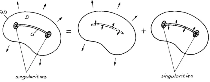
is forced to zero. This loading on the crack faces will generate another state of stress in the body, denoted by ~1.

T_hus, the solution to the problem of a cracked body can be obtained by superposition of ~1 on ~0:

L(x) = ~0(x)

+

L:1(x)

where ~0(x) is a regular stress tensor and ~1(x) is a singular one in the vicinity of the crack edge

as

(Fig. 1 ).

This leads us to consider what is called the auxiliary problem stated as the problem of a crack under arbitrary loadings. The boundary conditions are:

'fl X E S: lim t ( X, n x ) = - tO (X O , n x

J

(

1) x- xl, nx=n.,₀

'

I

+

smgularlt rf2!5 .s/ngular;t/es

Figure 1. Analysis of the problem of a cracked body.

In fact, one begins to obtain a solution to the problem with the boundary conditions (1) and another one slightly different from (2):

'V x,

II

x

II

~ oo : t ( x, n

x)

=

0 ( 2bis) The corresponding solution is rather satisfactory in the case of a little crack embedded in a large body. Nevertheless, if the crack is not sufficiently far away from the boundary

oD

of the body (especially in the case of surface and through cracks) use must be made of an appropriate method for satisfying the boundary condition (2). This method will be illustrated in the example at the end of this paper.

4. Integral equations for the auxiliary problem I) Definition of the displacement field

Let us represent the displacement field by means of the double-layer potential of the first kind of Kupradze [7]:

\fxEE₃(insteadof D): u(x)= JJf(x) = fsrT(y-x, ny).f(y) dSY (3) where the density .f is a vector function of three variables

z

= (

z _1, z _{2 ,} z ₃) defined on an open set {} containing S. Its .restriction on

S"-'

₁s(Z) ="-'(yES) satisfying the condition:

tJ!,s

E C1·a(S), 0 <a~ 1, is the unknown of the problem.

It is proved in

[71

that u(x) thus defined satisfies the homogeneous static Navier's equation:

leu= p.du

+

(A+

p.)

grad div u = 0, '::!x E £₃ \S (4)

It must be stated that the stress state generated by this displacement field satisfies the boundary condition (1), the condition (2bis) being identically satisfied.

Following [1]; we have a relation on limit behaviour of the displacement:

u( xl) =

±

i.f(x_{0 )}

+

pv

fs

TT( y - x₀, ny)t/1( y) dSY' 'Vx₀ E S

where:

(5)

r=r(z-x), e,=e,(z-x),

-

-T( y - x, n

y

)

= T(

z -

x, n

z

)

I

z =yes

Using (5), we obtain the displacement discontinuity on the crack:

[ u(x0 )]

=

u(xt)- u(x

0 )

= ljl(x0 ), ~x

0

E S (7) This discontinuity is thus directly related to the unknown density ljl( yES). Knowing ljl( y E S) will allow us to calculate, in particular, the stress intensity factors.

2) The state of stress

Since the boundary conditions are expressed in terms of stresses, we have to derive the expression of the stress from the displacement. According to (3), we have:

'V X E £3: t (X' n

J

=

.r

(ax' n

J

u (X) =

.r

(ax ' n

J

IsT

T ( y - X' n y)

~

( y) d Sy ( 8)

where ff(ax, nx) is the stress operator:

ff(ax,

n

x

)=2~tdd +~tn

x

Arot+An

x

div=c

iJk

t·n

1

(x)

.

a

0 (9)

nx

x

,

where:

ciJkt = A~iJ.~kt

+

~t( ~ik·~JI

+

~it·~ki) (10) Let the Green's tensor of the Navier's

Kelvin-Somigliana tensor):

operator be E(z - x) (also identified as

= 1 = 1 E (

z -

x) =

(A

) ( (A

+

3~t)

I+ (A

+

It)

e,

®

e,) .

-87T~J,

+

2~t r Where: e,=e,(z-x), r=r(z-x) By denoting:

U(ei, z- x) = E(z- x).ei We have [7) (see notations of (4)):

.ft?U(ei, z- x) = -~R3(z - x).ei

where ~R3(Z -x) denotes the Dirac measure concentrated at the point

z.

On account of the equality:

T(z- x

,

nJ

=ff(az,

n

z

)E(z-

x),

(11)

(12)

the stress vector at a point x, with respect to the normal n x can be rewritten in the form: t(x,

n

x

)

=ff

(o

x,

n

x

) ( [

ff(az,

n

z

)E(z-

x)]

rL

:

=

y

·~(

y) dSF

~ - (13)

i.e., for the /-component, using:

a£ . a£ .. - ' 1 (z - x)= - -11(z- x)

a

xk

a

z

k

(14)

where:

z=yES

Since EkJ has a point singularity of the type

,

-

1,

the kernel of integral (14) has a singularity of the type r- 3. This prevents us from applying the theorems on the limit

behaviour of double-layer potentials. Therefore it is necessary to perform some additional transformations so as to obtain afterwards a kernel of the type ,-2. This will be achieved

by using the Stokes theorem:

f rotza( y ).ny dSY =

1

a( y) d/Y

ls

as

where rotz implies that the derivatives must be performed with respect to the variable z;:

rotza( y)

=

rotza(z)

I

z=yES

and d~v is the contour element vector: d/Y = dy;.e;.

Setting:

a(z)=[(z).a0

where a₀ is some arbitrary constant vector, we obtain:

f grad z

I

A n y d

s

y

=

-A:.

!

d l.

ls

~s

i.e., for the m-component:

Multiplying both sides of (15) by £msp and taking into account:

we arrive at the following relation:

Setting here:

j(z) =1/;;(z).EkJt(z

-x)

,

we obtain:

(15)

(16)

[ o/;nsEkj tr dS = [

K~

5

.

Ekj

1 dS

+ [

o/;nrEkj,st dS

+

r/:.

£msro/;Ekj,t dym (17)

ls

·

ls

·

ls

'Yas

where K~s is defined by:

Substituting (17) in (14) gives:

Now in virtue of (10) and (12):

C;sktEkj,st = p,Eij.ss + (A+

p,)

Ekj,ik = ej . .ffU( e;' y - X) = - 8ij·8R" ( y - X) = 0

since x $. S, we eventually obtain:

f

i aEkj

t1

(x, nx)

= -c1p1rcisktnp(x)

_s

"rs·-:~-( _vz, y- x) dSr

+clpjrcisklnp(x)tf. EmrslJliEk) r dym

'Jlas

.

which gives, after performing all summations:

p,np(x)

f

1 ; t1(x,

n

x

)

= ( ) 2 {4v81pK;kr.k 8'17' 1 - v s r where: + (1 - 2v) [

K~pr

.

1

+

K;

1r.p

+

r.k (

K~k

+

Kfk))

+

3r.ir.k (

K~k r,~

+

K~k

r.p)} dSP

X [ f.rn;pr.l

+

f.rnilr.p

+

r.k ( f.mpk8il

+

f.mlk8ip)]

+

3r,,r.k ( f.mpkr.l

+

f.mlkr.p)} d Yrn

r=r(y-x), r

_.}

. _ar(z-x) = --'---

_az

-'--I :=yES

(19)

Thus, the stress vector is written as a sum of surface and line integrals, the kernel of surface integral is singular as r- 2. Next we will pass to the limit as

x-+ xl,

the limit

behaviour of double-layer potential being now available. On the other hand, when passing to the limit, there is no singularity in the line integral, since we have assumed the surface

S does not include its boundary

as

(see §2 - Basic notations), so that ,-2 _{in the line}

integral remains bounded when x tends to x0 E S. However, for x0 close by the contour

as

,

numerical difficulties should be expected.

Starting from another point of view, V. Sladek and J. Sladek [6] obtained similar

equations where the displacement discontinuity [u] was involved instead of 1/1. Despite the

equality (7), there are more difficulties in formulating surface or through crack problems in terms of [ u }. This will be well illustrated in the example by the end of this paper. For embedded crack problems, these two points of view are equivalent. Moreover, in {6], the crack S is considered as a closed surface resulting from the union of its upper and lower faces

s+

and

s

-

,

so the line integral taken on the boundary

as

vanishes. On the contrary

S, herein considered, is regarded as a geometric surface through which the displacement field is subjected to a discontinuity.

For an embedded crack we have:

which is equivalent to, by virtue of (7):

~( y) =

o,

'Vy E

as,

thus the line integral vanishes, and this result is consistent with Sladek's equations. On the other hand, for a surface or through crack, we have:

3yEaS:[u(y)]

*o.

The line integral does not vanish on a portion L included in

as (

L may be the union of separate arcs of

as),

and it is reduced to a line integral taken along L. As mentioned before, the kernel of the line integral is not singular, we shall denote it for simplicity:

5. Integral equations

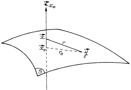
Formula (19) will allow us to express the boundary condition (1) in terms of stresses. For this purpose, the limit of the /-component of stress t1(x, nx) as x ~ xl and nx = nxo• x0

E S, is investigated (Fig. 2).

As was mentioned previously in §2 - Basic notations, S is a Liapunov surface, i.e. belonging to the class yl.a, 0 <a~ 1. Moreover,

-f

₁s was assumed to belong to the class

Figure 2. Case when x -+ xt and n x = n.x

0

cLa(S)

c

C0·a(S). Then one can prove the following formulae, valid for any point x_{0 E} S: e(y-x)®n lim

f

r 2 Y

l/1(

y) dSY x-+x± n =n Js r (y-x) 0 ' X Xo (20a) e (y-x) n lim

r

r 2 . y

tP ( y) d

s)'

x->x± n =n _{0 '} Js r

(y-x)

X Xo (20b) (20c) It should be noticed that every function occuring in the left-hand sides of (20) is expressed in terms of y or ( y - x ), whereas that in the right-hand side in terms of y or

( y -x₀). One also remarks the discontinuity when passing to the limit as x ~ x!.

From (20c), we obtain by changing the indices /, p, a symmetric equation:

(20d) Moreover, setting I= p in (20c), we have:

(20e) Using (20), we easily obtain:

(21b)

(21c)

We recall that functions in the left-hand side of (21c) are reckoned at y or ( y-x),

whereas those in the right-hand side at y or ( y- x_{0 )}. On account of (21), the limit of the

stress vector t₁(x, nx) as x-+ xf, nx = nxo' can be written in the form:

One can easily verify that the first bracket is identically zero, so that the limits as

x-+ xt and x ~ x

₀

coincide. This "continuity" is predicted by the Liapunov-Tauber

theorem (see for instance [7] or [8] as well). It should be noticed that the line integral on L is not singular. We eventually arrive at the following formula:

where t₁(x_{0 ,} nx

0) is understood in the sense of a limit, and:

K;d

y)

= n;(

y).IJ;i

.

d

y)

-

nk( y)l/;iJ(

Y)

r

=

r( y- x0 ) =

II

Y- Xo

II

ar(z-x)

ar(z-xo)

r = = - - ' - - -....::...;.._ , i - dZ z=yES

az

' x=xQES I z =yES (22)

For calculations in curvilinear coordinates (e.g. in cylindrical or spherical coordinates) it should be interesting to write (22) in the tensor form. Without more details, we give the

final result:

t(x_{0 ,} nx ₀ )=

(JL

)pvf

_!_

₂ {4v(nvgrado/er-(nver)div \fl)nx

8w 1-v lsr · · 0

+ [

(1- 2v)(nygradtftnx₀ - (nynx

0) div

t/1)

+

3(nynx

0

)ergrad~er

- 3(nyer)(

ergrad~nxJ]

er

+ [

(1- 2v )( nxogradtfter- (nx₀er) div

o/)

+

3(

nxoer )ergrad..J;er] ny

+

(1 -

2v) [ ( n xlr )gradT o/ny

+

(nynx₀)gradtfter-

(nyer)grad~nx

0

-

(nyer)gradTtftnxo] - 3(nxoer)(nyer)gradT..J;er} dSv

- (Jl

)j_!_

₂ {4v[\fl(erAd/)]nx

+

{(l-2v)[(l/1Anx )dl]

8w 1 - P L r 0 0

+

3[ n xJ erA dl)] ( ertft)} er

+

(1 - 2v) [ nxo (erA d/)] 1/1

+

(1 - 2v )(ern xo) d/A..J;

+ [

(1 - 2v )( 1/ln xJ

+

3( er1/l )( ernxJ] erA d/ (22bis) In the left-hand side of (22) and (22bis), the stress vector t(x₀, nx

0) is known for each

point x₀ E S. The derivatives lJ;;J( y) appear in the right-hand side, these are the derivatives of the function

o/

with respect to three independent variables z₁, z_{2 ,} z_{3 ,}

reckoned at a point yES. In fact, since the restriction of 1/1 on S is the unknown of the problem i.e.

o/(

y) for yES, one must prove that these t/;;J are actually reduced to the derivatives of the restriction of

o/

on S, with respect to some suitable variables.

Let a parametric representation of S be: F_{1 (} u, v)

(u,

v)E~o---)yES=F(u,

v)=

F₂

(u

,

v)

FEC1_·a(~)

(23)

F₃

(u,

v)

where~ is a domain of R2 and the components of Fare given in Cartesian coordinates.

The parameter u must not be confused with the displacement. For a point z of £₃ close to S, let us consider the coordinate transformation defined by:

z

1 F1

(u,

v)

+

w.n1

(u,

v)

z E £₃ = z ₂ = F_{2 (} u, v)

+

w. n ₂ ( u,

v)

(24) z₃ F₃(u,v)+w.n₃(u,v)

where ny(n_1, n2 , n3 ) is the normal to S at the point yES represented by the couple

(u, v). Since S E cLo:, 0 <a~ 1, every point of Sis a regular point, and F.u and F.u are linearly independent, so n Y is well defined:

n1(u, v)

ny= n2(u, v)= F.u(u, v)AF.1

,

(U

,

v)JllF.u(u, v)AF.o(u, v)ll

(25)

n

₃

(u,

v)

The function l/;(z) for z E £₃ is written in the form:

o/(z) = o/(z_{1 ,} z₂, z_{3 )}

=

l/1 (

F1 ( u , v )

+

w. n 1 ( u, v ) , F2 ( u , v )

+

w. n 2 ( u, v ) ,

F3

(

u , v ) + w. n 3 ( u , v ) ) .

The restriction of lf! on S is then:

The unknown of the problem is </»( u, v )~ it is to be proved that only the derivatives of cp( u, v) with respect to either u or v actually appear in the right-hand side of (22) or (22bis). We have: C/>;_u{u,

v

)

cf>;,u(u, v)

a·'·

·

-_an "''( ES) _y z F2.u(u, v) F2

,

v

(u

,

v)

F₃,u(u, v) F₃.v(u,

v)

l/1

;,

1 (yES) 1/;; ,2 ( y E

S)

(27) dl/;;(Z) We recall that: lj;i.J( yES)=

oz

.

} z=y ES

The system (27) can be inverted since F,u• F.v and n are linearly independent, the determinant of the system is equal to: (F.u, F.v• n)

=II

F.uAF,v

II·

We obtain:

t/-'

;,

1(yES) An A12

n

1 $;u(u,

v

)

t/-'

;

,

2(yES) _ A21 A22 n2 cf>; v(u,

v

)

a·'

·

·

A31 A32 n3 a:'(yES) z {28) Thus: (29) where the parenthesis does not include

:~

;

(yES}, but only cf>;,u and cf>;,v· From (29), we

z

hav~..;.

dl/1

(grad z

\f ) (

y E s)

=

grad z &Y ( z )

I

~

-

y E s = an z ( y E s ) ® n y

+ ( ..

.

)

(30a)

and:

(divz.Y )(yES)=

divz~(z)

I

~~

yES=

: : ( Y E S).ny

+ (

.

.

.

)

z

(30b) Using the relations (30a) and (30b), one can easily verify that

~t/1

(yES) are actually

unz

not involved in the kernel of the surface integral of (22) and (22 bis). As was expected, only the derivatives of the restriction of &Y on S, C/>;,u and $;,v• appear in (22) to (22 his).

This point is important for the effective resolution of the integral equations.

Finally, in the usual case when

F.u

is perpendicular to F.v• one can obtain from (22 bis) the integral equation for a general crack:

!l ( 1 1

t(xo, nxo)= 87T(1-v)pvJs"'? . IIR,uii·!JF.v \1.

{ 2( «P.u, e, F,v

)n

xo- (1 - 2v )( «P.u, en n xJF.v- (1 - 2v )( F.v · n xJ «P,u 1\ er

+3(er·fP.u)[(F.v, nxo• er)er+(nxa·er)eri\F,v]

- 2( «P.v• e,F,Jnx₀

+

(1- 2v )( «P.v• e, nxJ F.u

+

(1- 2v )( F.u · nxJ«P.v 1\ er

-3(er·4>,v)[(F.u, nxa• er)er+ (nxa·er)eri\ F.u]} dSy

( J.L )

J

~

{2(

i ', e, dl)nxo

+

(1-

2v )[ ( e, '1', nxJdl

+ (

dl· nx0)er 1\

'~']

87T 1-v Lr

{ +

3 ( e r · 'I') [ ( n x ₀, e, dl) e r

+ (

n x

6. Particular case of a plane crack

Let us consider a crack lying in the plane P (Fig. 3). A natural choice of the coordinate system is so that e₃ is the normal orientating P, and e_{1 ,} e₂ lie in the plane. We may choose the following parametrization of S:

FI ( u, v) u YI

y E S = F(

u, u)

= F2 (

u, v)

=

v

= Y2 F_{3 (}

u, v)

0 y₃ = 0 which obviously yields:

F. u = ( 1, 0, 0), F. v = ( 0, 1, 0) and n ( u, u) = ( 0, 0, 1) = e ₃ From (26), the restriction of ljl on S is:

cp(yl, Y2)

= ljl(yl, J2,

0)

According to the former discussion, the normal derivative : : (yES)=

~.

3

(y

1

,

y_{2 ,} 0) z

will not be involved, only the derivatives of the two-variables function

4>

remain: As:

<P;,I(YI> Y2) = tPi.l(Yl• Jl, 0) and <P;,2(Yl,

Y2)

= tPu(Yl• Y2• 0)

e r = ( r ,I , r ._{2 ,}

0)

ny = nx₀ = e3 = (0, 0, 1)

erAdl= sin 8. dl.nxo' (J

=

(er: d/) nx₀(erA d/) =sin 8. dl

(22ter) is reduced to the following in a Cartesian coordinates system: 1 2[(1-

2v)(<Pur

.

2 -<P2.2

r.l)

+

3r.1r.a<Pa./3r._{13 ]} r t(x0 , nxJ =

S7T(; _

v) pv

is ,\ {

(1-

2v )( cf>2.1r.1 - <P1_1r,2)

+

3r.2r,a<Pa,J3'.fJ]

(31)

2 p.

f

1

87T(l -

v)

L

r

2 2<P3,ar,a. r

[ (1 - 2v )( cf>An

x

J

dl

+

3(

ercf>) sin 8 dl] r.₁

+

(1 -

2v) sin 8 d/cp₁

[(1

-

2v){cpAnx

₀) d/+ 3(er<P) sin (J dl] r.₂

+ (1-

2v) sin 8 d/4>₂

(1 + 2v )( <PnxJ sin 8 dl + (1- 2v) sin 8 dlcp₃

where the Greek indices take the value 1 or 2.

--

e.3

11.::ro

-

a) In the case when the crack is embedded in the body, the line integral vanishes, the surface integral taken on S only remains. The third equation of (31) is visibly identical to that of Bui [4]. Let us prove that the first two equations are also equivalent to those of Bui.

We make use of the formulae of integration by parts:

j

J

l/;c/>,1 dy1 dy2 = -

j j

lfi.1cf> dy1 dy2

+

¢l/;ct> dy2

(32)

J

j

l/Jc/>,2 dy1 dy2 = -

J J

lfi.2cf> dy1 dy2-

¢l/Jct>

dy1

Having in mind that (22ter) involves a principal value, the surface integral in (32) must be performed overS except a circle a(x_{0 ,} £)with centre at x_{0 ,} the radius £ of the circle tending to zero; the line integral in (32) must be for the same reason taken along the boundary of a(x_{0 ,} £). By these formulae, one may prove for instance:

(33) p. f1 p.A t 1 ( Xo' n X ) = -4 pv 2 c/>1 ar a d Sy

+

(

i\ 2 ) o 7T s r . . 47T

+

p, pv

is

r\

r,~

(

cJ>11

+

cJ>2.2)

dSY (34)

which is identical to that of [4J.

It should be noticed that in this case of plane cracks, the mode I is uncoupled from modes II and III.

b) In some special problems, the density could take the form:

-/1 = (0, 0, t/;3) = l/;3.nxo

The first two equations are identically satisfied, as to the third one, it is reduced to: /l

r

cf>J.a'.a /l

r

c/>3 sin()

t3(xo, nxo) = 47T(l- P)pv Js r2 dSY - 47T(l- v) JL r2 dl (35)

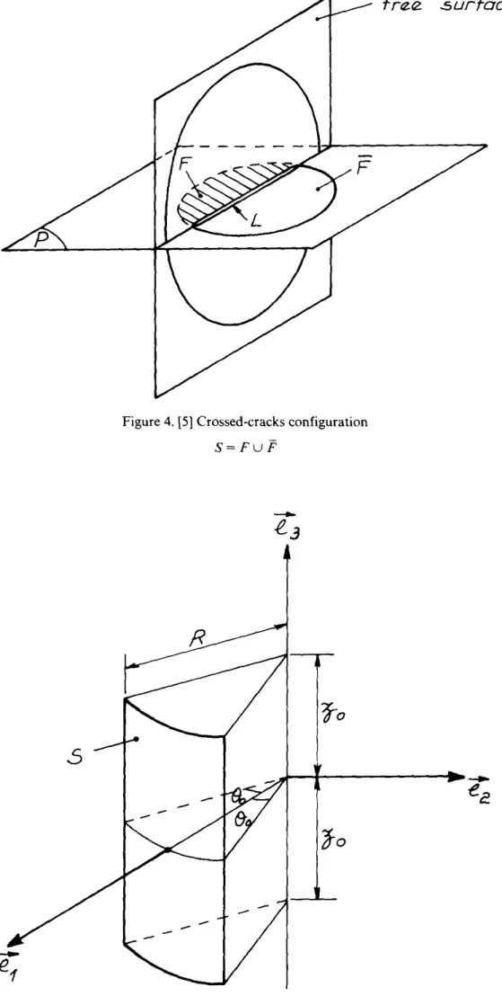
Putot studied in [51 the plane crack at a free surface in opening mode and obtained a system of equations without the line integral: he has considered the crack S made of the union of the surface crack Fin question and its mirror image

F

through the plane of the free surface (Fig. 4). The sy~etry of the problem, in particular the fact that t/;3

successively defined on F and F takes the same value at each point of L whereas the

associated line integrals are taken along opposite directions, implies that the line integral vanishes. When the free surface is not plane, a mirror image is meaningless and the line integral differs from zero.

7. Particular case of a cylindrical crack

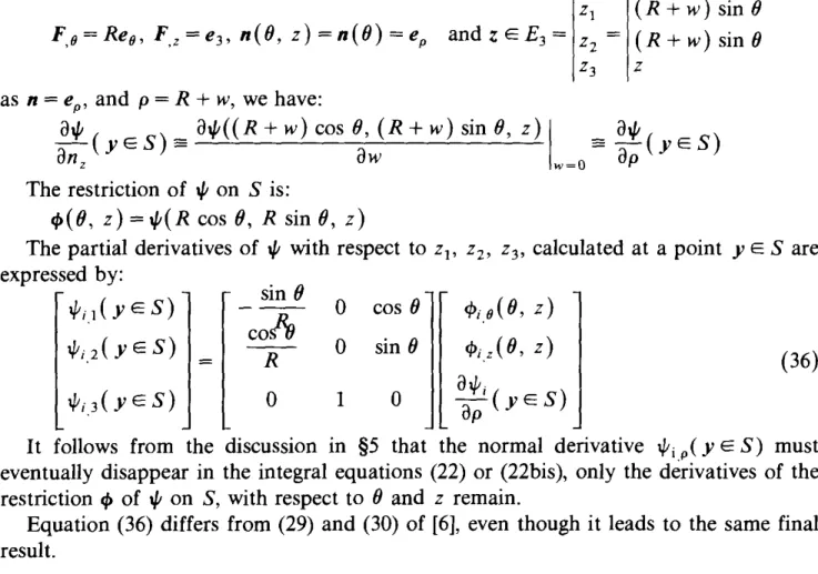
Use will be made in this section of cylindrical coordinates (p, 8, z). Let us consider a

crack curved in the shape of part of a cylindrical surface (Fig. 5), defined by:

112

+

yf

= R2 = const., ()

E]-

0_{0 ,} 8_{0 [,}

z

E]-

z

0 ,

z

0 [.

Following the notations of (23) to (30), we may choose a parametric representation of

S:

F₁ ( (), z ) R cos ()

y E S

=

F( (),

z)

= F₂ ( (),

z)

=

R sin 0

Figure 4. [5] Crossed-cracks configuration

S=FUF

-

.e3

Fnz.e .surfacrz

which yields:

z ₁ ( R

+

w ) sin () F,9=Re8 , F,z=e3 , n(O, z)=n(O)=eP andzEE3= z₂ - (R+w)sin()

z

3

z

as n = eP, and p = R

+

w, we have:

a

t/1 (

) _

a~

( (

R

+

w)

cos 8, ( R

+

w)

sin 8,

z)

I _

a~

(

)

- yES = = - yES

anz

aw

w=O

ap

The restriction of .f on S is:

cf> ( 8 , z )

=

tJl (

R cos (), R sin () , z )

The partial derivatives of ~ with respect to z_1, z_{2 ,} z_{3 ,} calculated at a point yES are expressed by:

tJ;i.

1

(yes)

t/;i2{yES) lj;i3(yES) sin ()

-cosRo

R 0 0 0 1 cos 0 sin 0 0

cf\

9

(0,

z) «Pi z ( (J'

z)

a.,,

_'Y, ( E

S)

ap

Y (36)

It follows from the discussion in §5 that the normal derivative lj;i p( yES) must eventually disappear in the integral equations (22) or (22bis ), only the derivatives of the restriction cf> of ~ on S, with respect to () and

z

remain.

Equation (36) differs from (29) and (30) of {6], even though it leads to the same final result.

8. Problem of a through crack in a cylindrical thick tube

Let us consider a cylindrical tube with the axis e_{3 ,} its outer and inner faces are ~₁ and ~₂

respectively, the tube contains a through crack S lying in a cross section (Fig. 6).

5 I I I

,_-

-

-

-.,- r .... / /

,

_____

... ~

___

_ . . / i

Let:

L1 = L1

n

S L₂ =

L

₂

n

S

L= L₁ U L₂

It is assumed that the tube is infinite along the e3-axis, that L1, L2 are free surfaces, and the crack is subjected to the prescribed loading t(x_{0 ,} nx₀ = e_{3 ).}

Let the surfaceS be oriented by e_{3 .} One can imagine that the two faces L_1, ~_{2 are also}

two crack surfaces, and these three cracks S, L_{1 ,} L₂ are imbedded in an infinite elastic medium. Let us define the displacement field as the sum of three double-layer potentials (cf. (3)):

\fxER3

:u(x) = Jrr(y-x,

n

y

)"'

1(y)

dSy+

J

...

Y.r(y-x,

n

y

)"'

2(y)

dL

Y

s

~1

(37)

where _{ny=e3 for} yES, n =eP for yE~₁, ny= -eP for yEL_2.

The densities "'1, "'2,

"'i'

are defined on three open sets containing respectively S, L₁

and ~₂; their respective restrictions constitute the unknowns of the problems. The boundary conditions are to be specified separately:

a) on the crack surfaceS: for each point x₀ E S, the prescribed tension t(x_{0 ,} nxo = e_{3 )} must be in equililbrium on the one hand with the stress, (31), yielded by the density l/;1

on S, on the other hand with the stresses, (19) yielded by the densities

tfl

2,

t/1

3 on ~

1

and ~

2

respectively. The associate integral equation has the form:

(38a) where the brackets [ ], too long to be explicit, stand for the kernel of (31).

b) on the free surface ~₁: for each point x₀ E ~h the sum of the stress generated by

"'2 on ~

1

,and those by "'1 on S and l/;3 on !._{2 ,} is equal to zero. This gives the second

integral equation which has the form:

Vx0 EL1

\

L

1:pv1 [ ... ]

d~

y+

ff(ax,

nx=eP)

~1

(Is

TT

>/-1 dSy

+

~'

TT

>~-' d~,) ~

0

(38b)

The first integral given by (22ter) involves now the density tf!2, we notice that there is

no line integral associated with the integral over L_{1 ,} the free surface being assumed to be infinite along the e3-axis.

c) on the free surface ~₂: by the same way we obtain the third integral equations:

'Vx0 E "'2.2

\L

2:pv 1 [ ... ] d!.>' +ff(ax, nx = - eP)

~2

( fsTT

.j-1 dSy

+

~'

TT

.j-2

d~

y

) ~

0

(38c)

Equations (38a) to (38c) constitute the integral equations system of the problem. The coupling between the crack S and the free surfaces is well illustrated.

For numerical purposes, let n_{5 ,} n~

₁

, n~

₂

be the respective nodes numbers on S, 2:_1, 2:_{2 ,}

there are 3 (n₅

+

n~

₁

+

n~) unknowns which are the values of l/;i/S at the nodes.

At each node, the prescribed stress is given, thus the system (38) becomes an algebraic equation system with 3 (n₅

+

n~

₁

+

n~) equations.

9. Conclusions

In general cases the derived integral equations system involves both surface and line integrals. Whereas Bui used two Kupradze potentials, a simple-layer and a double-layer, we limited ourselves to only one double-layer potential by analogy with V. and J. Sladek. The latter generates a point singularity of the type r-3 that we then transformed into a point singularity of the type r-2, after which we were able to utilize known results of

double-layer potentials.

We also demonstrated integral equations are not ill-conditioned, i.e. although the unknown density 1/1 was formerly defined on an open set containing the crack, only the restriction of 1[1 and its derivatives with respect to suitable variables appeared in the final integral equations.

By extension of Putot's point of view according to which a free boundary can be considered as an unloaded crack, we dealt with the problem of a finite body containing a three-dimensional arbitrarily shaped crack. It can be a through or a part-through crack. The example tackled in the last section, devoted to the coupling between a crack and free boundaries, showed that the same reasoning can be applied to more general cases

including the particular one of an inclined surface crack.

Numerical applications are being investigated. The relevant main difficulty is the computation of the singular surface integrals taken in the sense of the Cauchy principal value. Another difficulty results from the presence of free boundaries which increase both the size of the equations system and the number of unknowns.

References

[1J I.N. Sneddon, Proceedings of the Royal Society of London 187 (1956) 229.

[2] T.A. Cruse, International Journal of Solids and Structures 5 (1969) 1259-1274.

[31 V.D. Kupradze, Progress in Solid Mechanics, North Holland Pub. (1963).

[41 H.D. Bui, Comptes rendus de I'Academie des Sciences, Paris, t. 280, Serie A (1975) 1157, and H.D. Bui,

Journal of the Mechanics and Physics of Solids 25 {1977) 29-39.

[5] C. Putot and H.D. Bui, Comptes rendus de I'Academie des Sciences, Paris, t. 288, seie A (1979) and 311. C. Putot, Advances in Fracture Research, Pergamon Press, Oxford & New York (1980) 141.

(6] V. Sladek and J. Sladek, International Journal of Solids and Structures 19 (1983) 425-436.

[7] V.D. Kupradze, T.G. Gegelia, M.O. Bashelishvili and T.V. Burchuladze, Three-dimensional Problems of the

Mathematical Theory of Elasticity and Thermoelasticity, North Holland Pub. (1979).

[8] V. Parton and P. Perline, Equations lntegrales de Ia Theorie de I'Eiasticite, Nauka 1977, translated from

Russian (1983).

Resume

A l'aide des potentiels de Kupradze on formute sous forme d'equations integrates le probleme d'une fissure tridimensionnelle dans un solide fini ou non. Le solide a un comportement elastique lineaire homogene et

isotrope et la fissure peut etre debouchante ou non ou meme traversante. Dans les equations finales apparaissent

dans le cas general a la fois des integrates de surface et des integrates curvilignes. Pour une fissure debouchante, !'integrate curviligne est prise sur une portion du front de fissure. Pour une fissure plane, immergee, on retrouve les equations integrales developpees par Bui. Une autre application concerne le cas d'une fissure traversante dans un tube circulaire.